Modélisation des réserves en assurance I.A.R.D. : utilisation de méthodes robustes

UNIVERSITÉ DU QUÉBEC À MONTRÉAL

MODÉLISATION DES RÉSERVES EN ASSURANCE I.A.R.D. -UTILISATION DE MÉTHODES ROBUSTES

MÉMOIRE PRÉSENTÉ

COMME EXIGENCE PARTIELLE DE LA MAÎTRISE EN MATHÉMATIQUES

PAR

ZAHRA GHASEMIVANANI

UNIVERSITÉ DU QUÉBEC À MONTRÉAL Service des bibliothèques

Avertissement

La

diffusion de ce mémoire se fait dans le respect des droits de son auteur, qui a signé le formulaire Autorisation de reproduire et de diffuser un travail de recherche de cycles supérieurs (SDU-522 - Rév.1 0-2015). Cette autorisation stipule que «conformément

à

l'article 11 du Règlement no 8 des études de cycles supérieurs, [l'auteur] concède à

l'Université du Québec à Montréal une licence non exclusive d'utilisation et de publication de la totalité ou d'une partie importante de [son] travail de recherche pour des fins pédagogiques et non commerciales. Plus précisément, [l'auteur] autorise l'Université du Québec à Montréal à reproduire, diffuser, prêter, distribuer ou vendre des copies de [son] travail de recherche à des fins non commerciales sur quelque support que ce soit, y compris l'Internet. Cette licence et cette autorisation n'entraînent pas une renonciation de [la] part [de l'auteur] à [ses] droits moraux ni à [ses] droits de propriété intellectuelle. Sauf entente contraire, [l'auteur] conserve la liberté de diffuser et de commercialiser ou non ce travail dont [il] possède un exemplaire.»

---

-~---.-Writing this note of thanks is the finishing touch on my dissertation. It has been a period of learning for me, not only in the scientific area, but also on a persona! level. Writing this dissertation has had a big impact on me. 1 would like to reflect on the people who have supported and helped me so much throughout this period. First, 1 would like to thank my supervisor Professor Mathieu Pigeon, 1 want to thank you for your excellent cooperation and for aU of the opportunities 1 was given to conduct my research and further my thesis. In addition, 1 would like to thank aU my tutors, for their valuable guidance. You definitely provided me with the tools that 1 needed to choose the right direction and successfully complete my thesis. Moreover, 1 want to thank Mrs Gisèle Legault who helps me to solve the software and hardware issues 1 have had.

1 would also like to thank my mother for her support and sympathetic ear. You are always there for me. Finally, there are my friends. We were not only able to support each other by deliberating over our problems and findings, but also happily by talking about things other than just our papers.

LIST OF TABLES . LIST OF FIGURES RÉSUMÉ .. ABSTRACT INTRODUCTION CHAPTER 1 ROBUST STATISTICS

1.1 Introduction and Motivation . 1.2 Measuring Robustness . . . .

1.2.1 Empirical Influence F\mction 1.2.2 Influence Function 1.2.3 Breakdown Point . 1.2.4 Qualitative Robustness . Vll ix xi xiü 1 5 5 9 10 12 17 19 1.3 M-Estimators . . . 21 CHAPTER II

CLASSICAL MODEL FOR RESERVE IN GENERAL INSURANCE 29

2.1 Introduction and Motivation . . . 29

2.2 Collective and lndividual Approaches . 31

2.2.1 Collective Approach 31

2.2.2 Individual Approach 34

2.3 Generalized Linear Models . 34

2.3.1 The (Over-dispersed) Poisson Model for Loss Reserving . 40

2.4 Stochastic Chain-Ladder Model 46

vi

2.5.1 Influence Function for the Generalized Linear Model for Reserves 56 2.5.2 Influence Function for the Stochastic Chain-Ladder Model 57 CHAPTER III

ROBUST PROCEDURES IN LOSS RESERVING MODELS 3.1 Robust Generalized Linear Models . . . .

69

69

3.1.1 The Structure of the Robust Poisson Model for Reserves 70 3.1.2 The Influence Function of the Robust Poisson Model for Reserves 72 3.2 Robust Version of the Stochastic Chain-Ladder Model

3.2.1 Robust development factor . . . . 3.2.2 The Structure of the Robust Chain-Ladder Model .

3.2.3 The Influence Function of the Robust Chain-Ladder Model for Reserves .

CHAPTER IV

CASESTUDY . . . .

4.1 Generalized Linear Model

4.1.1 Classic Generalized Linear Model 4.1.2 Robust Generalized Linear Model . 4.2 Stochastic Chain-Ladder Model . . . .

4.2.1 Classic Stochastic Chain-Ladder Model . 4.2.2 Robust Stochastic Chain-Ladder Model. 4.3 Percentile match . . . .

APPENDIX A

MATHEMATICAL DEFINITIONS APPENDIX B

GENERALIZED LINEAR MODELS B.1 Exponential family B.2 Caracteristics . . . B.3 Parameters Estimation . 77 78 79 88

93

93

94 95

96

96

98

100 105 111 111 112 113

Tableau Page 1.1 Statistics in presence and absence of an outlier for Example 1.1 10 2.1 Rate of payment in various tines of business. . . 30 2.2 Cumulative run-off triangle {in millions of dollars). 32 2.3 Cumulative run-off triangle from Taylor et Ashe {1983). . 43 2.4 Predicted incrementai triangle obtained from the classicai Poisson

model for loss reserving. . . 44 2.5 Predicted incrementai triangle in presence of an outlier, completed

with classicai GLM method. . . 45 2.6 Run-offtriangle {observed and predicted cumulative paid amounts)

with the stochastic Chain-Lad der model. . . 55 2. 7 Run-off triangle in presence of an outlier with the stochastic

Chain-Ladder model. . . 56 3.1 Cumulative run-off triangle from Taylor et Ashe {1983). . 74 3.2 Predicted incrementai triangle. . . 75 3.3 Predicted incrementai triangle in presence of an outlier. 76

3.4 Predicted reserves (c = 1.345). . . . 76

3.5 Estimated reserve with modified c. 77

3.6 Cumulative run-off triangle (in millions of dollars). 82 3.7 Evaluated run-off triangle (in millions of dollars). 83

3.8 Pearson residulals. 84

3.10 Pearson residuals . . . . 3.11 Occurred and predicted cumulative amounts. . 3.12 Full matrix in presence of an outlier.

3.13 Predicted reserve . . . .

3.14 Occurred and predicted cumulative amounts .. 3.15 Full matrix in presence of an outlier.

3.16 Predicted reserve . . . . 4.1 Incrementai run-off triangle. 4.2 Cumulative run-off triangle.

4.3 Predicted incrementai run-off triangle.

4.4 Reserve amounts using the Classic and the Robust GLM in presence viii

85

86 86 87 89

90

91

94 94

95

of outlier. . . 96 4.5 Detailed results with the classic stochastic Chain-Ladder model. 97 4.6 Development factors with the classic stochastic Chain-Ladder model. 98 4.7 Run-off triangle with Classic stochastic Chain-Ladder.

4.8 Predicted and observed cumulative payments. . . .

4.9 Reserve amounts with the classic and robust Chain-Ladder model 98

99

in presence of outlier. . . 100 4.10 Reserve percentile various models without outlier. 101 4.11 Reserve percentile in various with an outlier in position (2, 1). 101

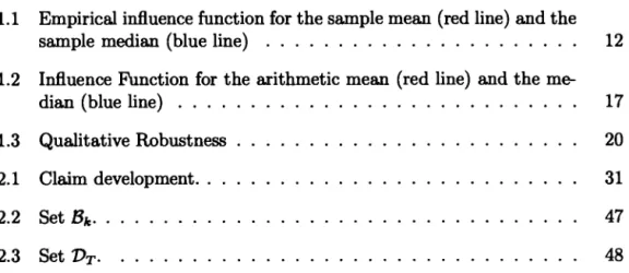
Figure Page 1.1 Empirical influence function for the sample mean (red line) and the

sample median (blue line) . . . 12 1.2 Influence F\mction for the arithmetic mean (red line) and the

me-dian (blue line) . . . . 17

1.3 Qualitative Robustness 20

2.1 Claim development. . 31

2.2 Set

Bk. .

47

Une police d'assurance reçoit une prime initiale et elle paiera les réclamations fu-tures probables. En conséquence, l'assureur ne connaît pas tous les coûts futurs, ainsi que le calendrier des paiements. Par conséquent, l'un des plus gros passifs de l'assureur est mettre un capital de côté afin de couvrir tous ces paiements futurs. Parmi toutes les méthodes de réservation existantes en assurance générale, nous considérons deux modèles dans ce travail: le modèle stochastique de la Chain-Ladder (ou le modèle de Mack Chain-Chain-Ladder) et le modèle linéaire généralisé (ou GLM) pour les réserves. La première est la technique la plus utilisée pour cal-culer la réserve actuarielle et l'autre s'applique à un large groupe de sinistres qui appartenant à la famille exponentielle. L'existence d'un outlier (ou des valeurs aberrantes) dans l'ensemble de données créera une réserve sous-estimée ou sures-timée pour les deux méthodes. Cette erreur de prédiction peut être grande et il

est essentiel de modifier ces méthodes de manière à ce qu'elles deviennent moins sensibles et plus précises, même en présence de valeurs aberrantes. Dans cette étude, nous présentons le cadre général pour des statistiques robustes, ainsi que nous expliquons les approches basiques dans la réserve de perte telles que le mod-èle stochastique de la chaîne et le GLM pour les réserves. Ensuite, nous étudions des versions robustes de ces modèles avant de passer par un exemple basé sur un ensemble de données réelles.

Mots-clés: Statistiques robustes, provisionnement des sinistres, assurance générale, modèle Mack Chain-Ladder, modèle linéaire généralisé (GLM).

Insurance companies receive an upfront premium and will pay future probable claims. As a result, the insurer knows neither the future costs nor the payment schedule. One of the largest liabilities of the insurer is therefore to put capital aside in order to cover ali these future payments.

Among ali existing reserving methods in general insurance, we consider two models in this work: the stochastic Chain-Ladder model (or Mack Chain-Ladder model) and the generalized linear model (or GLM) for reserves. The former is the most widely used technique to calculate the actuarial reserve and the latter is applicable for a wide range of claims which belong to the exponential family. The existence of an outliers in the dataset will result in an underestimated or overestimated reserve for both methods. This prediction error may be large and it is essential to modify these methods in a way that they become less sensitive and more accurate, even in presence of outliers.

In this study, we introduce the general framework for robust statistics, as weil as explain basic approaches in loss reserving such as the stochastic Chain-Ladder modcl and the GLM for reserves. We then study robust versions of these models before going through an example based on a real data set.

Keywords: Robust statistics, loss reserving, general insurance, Mack Chain-Ladder model, Generalized linear model(GLM).

The evaluation of future profit or loss becomes more and more important every day. The market is so competitive and only insurance companies with an accurate plan can survive. At each moment, an insurance company needs to put aside a sufficient capital amount in order to be able to pay ali future liabilities generated by the contracts that have been sold to the clients. This capital forms the reserve (or provision) of the non-life company. Periodically, insurance regulators require an evaluation on this reserve in order to control the financial solvency of the company and to protect policyholders.

For a very long time, aU calculations for evaluating loss reserve in insurance com-panies were done using simple deterministic algorithms. But since the early 1990s, actuaries have started to propose more sophisticated stochastic methods to man-age the solvency of the company.

Two of the most important methods for estimating the outstanding reserves are the stochastic Chain-Ladder model (or Mack's model) and the generalized linear model (or GLM) for reserves. The ultimate goal of these methods is to accurately predict the amount of reserve but, as we will see, both methods are highly de-pendent on the data. In fact, the stochastic Chain-Ladder model uses the daims history in order to predict future developments and the GLM for reserves uses daims history in order to estimate unknown parameters. Both approaches can quickly become inaccurate in case of existence of outliers.

An outlier is a sample value that is significantly different when compared with the majority of the sample. It is not necessarily a wrong value, but it should always

2

be checked for a transcription error. The existence of an outlier could have a large effect on the estimation procedure as well as on the total reserve amount. It could cause reserve underestimation or overestimation and problems in the solvency on the insurance company. This is a well-known issue in several areas and many robust statistical methods have been developed to be less sensitive to the outliers (see Wüthrich et Merz (2008)).

Since 1953, when Box fust gave the word "robust" its statistical meaning, this field has evolved considerably, although the concept already existed for several decades (see Stigler (1972) for more details).

Several persons consider that the fundamental work in robust statistics was done in the 1960s, and the early 1970s by Thkey (1960, 1962), Huber (1964, 1967) and Frank Hampel (1971a, 1974). One of the possible reasons for this significant development was the accessibility of modern and fast computers. From the early 1980s, robust statistics have experienced considerable growth and many of the most influential books in this field, such as Huber (1981), Hampel et al. (1986a), Rousseeuw et Leroy (1986) and Staudte et Sheather (1990), were written during this period. Several researches have appeared in recent years on applying robust analysis to loss modeling and to reserve evaluation. For example, see Gather et Schultze (1999), Wüthrich et Merz (2008) , Cantoni et Ronchetti (1999) and Verdonck et al. (2009).

Based on Maronna et al. (2006) and Hampel et al. (1986b), we introduce "robust statistics" and all related concepts such as M-estimator in the fust chapter. In the second chapter, we present two of the most important reserving methods in non-life insurance: the stochastic Chain-Ladder model (based on Wüthrich et Merz (2008)) the family of generalized linear models (GLM) for reserves. In this chapter, we also study how sensitive are these methods to outliers. As a solution of high dependency of reserve to outlier data, we introduce a "robustified" version

of both models in Chapter 3. The robust stochastic Chain-Ladder model is based on Verdonck et al. (2009) and Verdonck et Debruyne (2011), while the robust GLM is based on Cantoni et Ronchetti (1999). Finally, we go through a real study case in the Chapter 4.

ROBUST STATISTICS

In this chapter we introduce robust statistics and we present sorne measures of robustness such as the empirical influence function, the influence function and the breakdown point.

Robust means model's, test's or system's ability to perform effectively and without failure while its assumptions or variables altered or violated. For statistics, a robust model can still provides insight to a problem despite having its assumptions altered. It is expected the robust statistics gives more reliable results than classic statistics.

1.1 Introduction and Motivation

Statistics play an important role in reducing and organizing information provided in a dataset. For instance, the sample mean summarizes the "central tendency" of a sample to a single value. Robust statistics go beyond that by offering good performance even if sorne standard assumptions such as normality, linearity or independence are not thoroughly verified. For example, robust methods will re-main valid for samples drawn from a wide range of probability distributions and in particular from a non-normal distribution.

6

always be checked for transcription errors, measurement errors, etc. They can ruin standard statistical methods because in the presence of outliers, most of the statistics often used in practice become useless and traditional estimators, such as maximum likelihood estimators or moment-based estimators, have poor performance (see Maronna et al. (2006)). Thankfully, many robust statistical methods have been developed to be less sensitive to the outliers.

Let x= {x1,x2, ... ,xn} be a set of observed values. The sample mean

x

and the sample standard deviation s are defined by

The sample mean is just the arithmetic average of the data and, as such one might expect that, it provides a good estimate of the "center" or "location" of the data. Likewise, one might expect that the sample standard deviation would provide a good estimate of the "dispersion" of the data. N ow we shall investigate how mu ch influence a single outlier can have on these estimates often used in practice. Example 1.1. We considera portfolio with 24 payments in thousands of dollars, in ascending order:

2.20 2.20 2.40 2.40 2.50 2.70 2.80 2.90 3.03 3.03 3.10 3.37 3.40 3.40 3.40 3.50 3.60 3.70 3.70 3.70 3.70 3.77 5.28 28.95.

The maximum sample value, 28.95, is meaningfully laryer than the remaining

23 observations in the sample and the difference with its previous value {5.28) is

misplaced decimal point. The original value could have been 2.895.

We calculate the sample mean and the standard deviation which are

x

= 4.28 and s = 5.3. As we can see in the sample, there are only two observations above the mean which is an evidence for us to realize that the mean is not between the bulk of the data and it is not a good estimation of the central tendency of the data. After deleting the suspected outlier and re-calculating the sample mean and the standard deviation, we obtain

x= 3.21

and s = 0.69. The new mean is between the eleventh and the twelfth number, which is a more reasonable estimate of the center of the data. Also, the standard deviation is over seven times smaller than it was in the presence of an outlier.

To complete this introductory example, we are interested in the effect of any out-lier on these two statistics. We assume that the value of the outout-lier is replaced by a random variable X which can take any values between

-oo

and

+oo.

Conse-quently, the resulting sample mean will take values between

-oo

to

+oo.

Thus, we can say that a single outlier has an unbounded effect on the sample mean. Similarly, the standard deviation will take a positive value up to

+oo

and we can conclude that a single outlier has an unbounded effect on the standard deviation.

The above example shows that deleting outliers is a simple way to handle the problem but it may cause sorne problems:

• deletion is a subjective decision because the analyst has to decide when an observation is outlier enough to be removed from the sample;

• by removing sorne "extreme" points in the sample, there is a risk of under-estimating (or overunder-estimating) location and/ or dispersion; and

8 • eliminating sorne points from the sample may affect sorne properties of

statis-tics ( unbiasness, etc.).

As shown in the previous example, the sample mean and the standard deviation are not the best statistics, since they are highly infiuenced by outlirs. Fortunately, there are other options for estimating the central tendency and the dispersion of the data, for instance the median and the median absolute deviation. We rank the elements of a random sample (xl! x2 , •.. , Xn) in ascending order

and the sample median is defined by

. {X(m), med1an x = ( ) X(m)

+

X(m+l) 2 ' ifn = 2m -1 if n = 2m.

In the introductory example, the sample median for the original sample is 3.37, while the sample median without the outlier is 3.37. Moreover, when the largest value in the sample (28.95) is replaced by a random value in ( -oo, +oo) , the sample median does not change. As the median is not infiuenced by the presence of an outlier, we conclude it is a robust alternative to the sample mean. We say that the median is resistant to outliers whereas the mean is not. In fact, the median can tolerate a proportion of outliers up to 50

% before it becomes

arbitrarily large and useless. Formally, we could say that its breakdoum point is 50

% whereas the breakdown point for the mean is 0 %.

about the median (MAD) which is defined by

MAD(x)

=

MAD(x1, X2, ••• ,

Xn)

=

Median{lx- Median(x)l}.

In order to compare the median absolute deviation about the median to standard deviation, we define a "normalized" version of the MAD (MADN) as

MADN ( ) = MAD (x) x 0.6745 ,

where 0.6745 is the median absolute deviation about the median of a standard normal random variable. Indeed, we have

1

Pr[IZI

~y]=

2,

where y is the unknown value and Z ""'Normal(O, 1). Therefore we have

Since <1>

(-y)

= 1-<1>

(y),

we have

y=

<P-l

(~)

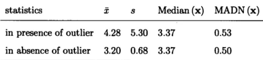
= 0.6745.

In the Example 1.1, the normalized version of the MAD is 0.53 for the complete sample and it decreases to 0.5 after deleting the outlier (28.95). It pointed out that the (normalized version of the) median absolute deviation about the median is not influenced very much by the presence of an outlier and provides a robust alternative to the standard deviation. For the Example 1.1, we present the full results in Table 1.1.

1.2 Measuring Robustness

The basic tools to describe and measure robustness are the empirical influence function, the influence function and the breakdown point which are defined in

10

Table 1.1 Statistics in presence and absence of an outlier for Example 1.1

statistics

x

s Median (x) MADN (x)

in presence of outlier 4.28 5.30 3.37 0.53 in absence of outlier 3.20 0.68 3.37 0.50

subsections 1.2.1, 1.2.2 and 1.2.3. These approaches are part of the field called

quantitative robustness in the literature (see Hampe! et al. (1986a) and Maronna et al. (2006)) because they really allow to measure the robustness of a statistic.

Conversely, we introduce in subsection 1.2.4 a different way to describe the ro-bustness of a statistic called qualitative roro-bustness. In the following chapters of this document, we mainly focus on the empirical influence function and the in-fluence function in order to measure the robustness of our estimators. Finally, mathematical definitions are gathered in Appendix A.

1.2.1 Empirical Influence F\mction

The empirical influence function is a measure of how a statistic is related to (or depends) a single point of the sample. This measure does not depend on the model since it simply relies on re-calculating the estimator with a different sample. In order to formalize the concept, we need1 a probability space

{0,

A,

JP>}

and two measure spaces {x,~} and {r,

S}.

We considera vector of independent and identically distributed (iid) random variables Xll ... , Xn, nE N, where

xi

:{n,A}--+

{x,~}.

A sample from these random variables is denoted by x= {x1 , ... , xn}· Finally,

we define a statistic

For the ith observation in the sample, the empirical influence function (EIF) of the statistic

Tn

is given by

EIFi : X --t lR

X

1---t n (Tn(Xi, ...

,Xi-i!

x, Xi+l1 • • • ,

Xn)- Tn(x)).

(1.2.1) The empirical influence function measures the amount of change in the statistic if we replace the ith observation by an arbitrary value x.

Example 1.2. We want to study the effect of a change of one of the observations

in the sample of the Example 1.1 on both the sample mean and the sample median by using the empirical influence fu.nction {note that 28.95 is present in the sample}. As a first step, we have randomly selected the observation x19 and changed it from

3. 7 to 6. 78. The new sample mean is

x

= 4.40 and for the sample median, the new value is 3.38. The value of the empirical influence fu.nction for the sample sample mean is

E/F1g(6.78)

=

24(T24(xl! ... ,xls,6.78,x2o, ... ,x24)- T24(x)) = 24( 4.40 - 4.28)

= 2.88

and for the sample median is

E/Flg(6.78)

=

24 (T24(x1, ... , X1s, 6.78, x2o, ... , x24)- T24(x))

=

24(3.38 - 3.38) =0.

12

This last value shows that the sample median is not affected when we replace the observation x19 by a different value.

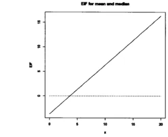
As a second step, we evaluate the empirical influence function for an arbitrory value x and we create the plot presented in the Figure 1.1. This groph shows that the EIF for the sample mean is unbounded, that is to say the impact of an outlier on this statistic can be huge.

EFfor _ _ _

10 15 20

Figure 1.1 Empirical influence function for the sample mean (red line) and the sample median (blue line)

1.2.2 Influence Function

The influence function (/

F)

is a measure of the dependence between an estimator and the model's distribution. It does not just rely on the sample data; instead, it considera the effect of a slight change of the distribution on an estimator. In arder to define the influence function in mathematical format we need to define sorne concepts.

Functionals

Let F8 be the parametric cumulative distribution function (edf) and fs be the corresponding probability density function (pdf). We need to find an estimator for the parameter (} based on a dataset. For a random sample

(X11 •.• , Xn),

we define the empirical distribution function

where

l(A)

is the indicator function of the event A. One should note that the empirical distribution function does not take in to account the order of the obser-vations.

An estimator of (} is

It means that (1)

Ô

can be seen as the sequence of statistics

{Tn;

n ~ 1}, one for each sample size n, and (2)

Ô

does not depend on the order of the observations. Estimators are functionals or can be replaced by functionals. It means it exists a functional

T:

Or~ lR, where

Or

stands for the domain of

T,

such that

(1.2.2)

in probability when the observation are independent and identically distributed according to the distribution G in

Or.

Moreover, we assume that the functional T is Fisher consistent, that is to say that at the true model

F,

the sequence

{Tn;

n ~ 1} measures asymptotically the correct quantity.

(1.2.3)

~---14 Gâteaux-derivative

The influence function is the limit of the Gâteaux derivative with respect to a smooth deviation, as the deviation approaches a point mass. The Gâteaux deriva-tive limit provides a way to calculate the solution to the functional equation, where the influence function appears as the limit of the Gâteaux derivative. In this way the Gâteaux derivative limit provides a way to circumvent the need to try to guess the solution of the functional equation.

We say that the functional T( G) is Gâteaux-differentiable at the distribution F

in

nT

if it exists a real function a such that

lim

(T((1-

t)F +tG)- T(F))

=

J

a( x) dG(x),

t--+0

t

(1.2.4)

The Gâteaux-derivative generalizes the directional derivative. In particular, if we choose G =~x' the empirical distribution which gives mass 1 tox, we obtain

~~

(T((1-

t)F

+/~x)-

T(F)) _

J

a(y)

d~x(Y)

- a(x). (1.2.5)

Here T( G) is the asymptotic value of the estimator sequence {Tn; n ~

1}

as mentioned above.

Back to the influence function

Remind that we aim at evaluating what will happen when the data do not follow the model F exactly but they follow a different distribution G. To do that, we want to evaluate the one-sided directional derivative of T at F, in the direction of G- F, i.e.

lim

(T((1-

t)F +tG)- T(F)).

t--+0

t

(1.2.6)

This last expression is true for all distribution GE

nT.

In particular, if we want to evaluate the contamination effect of a point x on the estimator, we may assume

that G =~x· Then, the influence function is defined by

IF(x;T,F)

=

lim

(T((l-

t)F+t~x)-

T(F)).

t--+0

t

If in Equation (1.2.5) we put G = F, we obtain

~~

(T((l-

t)F

~tF)-

T(F)) =

J

a(y) dF(y).

By putting together Equation (1.2.5) and Equation (1.2.8), we obtain

J

1 F(y; T, F) dF(y) = O.

(1.2.7)

{1.2.8)

In order to clarify the concept of influence function and the notation introduced before, we consider the influence function of the arithmetic mean. Let the sample space be

x=

1R and the parameter space be(}= 1R. We assume that the model's distribution is the standard Normal with probability density function

xE 1R,

the true value of the parameter is 00

=

0 and thus F90

=<P.

The arithmetic mean

is

and the corresponding functional for all probability measures with existing first moment is

T(G)

=

J

udG(u).

From Equations (1.2.3), we conclude that T is Fisher consistent

T(FtJ) =

j

udFa(u)

=

J

u(2n)-(1/2) exp-(1/2)u2 du

16 0 is the value of the parameter

e.

By using Equation (1.2.8), it follows that

IF(x·T F)

=

(lim

Jud[(1-t)~+t~x](u)- Jud~(u))

' ' t-tO t

=

lim ((1-t)

J

ud~(u)

+

t

J

ud~x(u)-

J

ud~(u))

t-tO

t

=

lim (0

+

tx -

0)

(1.2.9)

t-tO

t

because

J

ud~(u) =O. Therefore

IF(x;T,F) =x. (1.2.10)

Moreover, we assume that the asymptotic normality assumption is verified (see Hampel et al. (1986a))

fa(Tn-:n(G)) weakly N(O,V(T,G)),

n n-too (1.2.11)

where V(T, G) is the asymptotic variance given by V(T,F) =

J

IF(x;T,F)2dF(x). we will define IF(x;T,F) in equation (1.2.7).

Example 1.3. Suppose that the theoretical distribution of the data in Example 1.1 is the standard Normal. We want to evaluate the influencefunction of2 estimators for the location parameter J.L: the empirical mean

x and the median median(x).

Obviously the empirical distribution is different since mean and variance are not 0 and 1 respectively. In order to calculate the influence function for the functional Tn(G)

=

x,

we use Equation (1.2.10) which is the arithmetic mean's influence function for the standard Normal distribution. For the median, we have

It is easy to show that [1.

=

median(x)

=

3.38 in our example.

In Subsection 1.3, we show that the influence function of the median in this model is proportional to sign (xi - [1.). In this example,

sign(xi- median(x)) = sign(xi-3.38).

The Figure 1.2 illustrates both influence functions for some values of x. As it has been illustrated in the figure, the influence function for the mean seems to be unbounded and the influence function for median is bounded.

EFfor _ _ _

Figure 1.2 Influence Function for the arithmetic mean (red line) and the median (blue line)

1.2.3 Breakdown Point

The influence function, which describes the infinitesimal stability of an estimator, is a very useful tool for measuring the robustness but it has one major limitation: it is a local concept. Thus, it must be complemented by at least one more global

18

measure to assess the reliability of an estimator. This measure must show up to what "distance" from the madel distribution the estimator still gives sorne relevant information. The breakdown point of an estimator is the proportion of incorrect observations an estimator can handle before giving an incorrect result. The contamination should not be able to drive the estimator

Ô

to infinity, or to the boundary of the parameter space 9 when it is not empty, in order for the estimator Ô to give sorne information about 0.

The breakdown point e* of the sequence of estimators {Tn; n ~ 1} at the distri-bution Fis defined below. The evaluation of parameter is 800 as x goes to oo (x is a sample observation).

Definition 1.1. The asymptotic contamination breakdown point of the estimator

Ô at the distribution F, denoted by e*(Ô, F), is the laryest e* E

[0,

1) such that for e*

<

ê,

Ô

00((1-e)F+eG) as afunction ofG remains bounded, and also bounded

away from the boundary of

e.

We interpret the above definition in the following way: there exists a bounded and closed set K

c

9 such that K

n

De =

0 (

where De denotes the boundary of the parameter space e) and

Ôoo((1-e)F

+

eG) E K, 'Ve

<

e* and 'VG. (1.2.12)

As we illustrate in Example 1.1, changing (or removing) one observation in the sample has a large impact on the estimated value of th~ mean. If we replace the larger value in the sample by an arbitrary large value, we obtain an arbitrary large value for the empirical mean. Therefore, we conclude that the breakdown point for the sample mean isO. Conversely, the sample median showed sorne resistance to the modification of an observation. We conclude its breakdown point is larger that O. Actually, it is possible to show that the breakdown point of the sample

median in this example is 50

%,

which means it will be resistant up to 50

% of

contamination in the sample (see Maronna et al. (2006)).

The breakdown point is the smallest fraction of gross errors which can carry the statistic over all bounds. Somewhat more precisely, it is the distance from the model distribution beyond which the statistic becomes totally unreliable and uninformative. Finally, it measures directly the global reliability of a statistic. 1.2.4 Qualitative Robustness

We turn next to the definition of a global measure of the robustness of a statistic. This is, in sorne sense, a qualitative measure of the robustness of an estima tor. By qualitative, we mean a dichotomous measure (yes or no) of the robustness as opposed to a quantitative measure that evaluates the level of robustness of a statistic.

In order to define the concept of qualitative robustness, we remind the well-known definition of the continuity of a real-valued function.

Definition 1.2. Let 1 be an interoal in R and f : 1 --t R be a fu.nction. f is a continuous function at

o:

E 1, if\/€

>

0 there exists ~

>

0 such that \lx E 1, we have

lx- o:l

<

~

=>

IJ(x)-

f(o:)l

<

f.

Now, we generalize this definition to the case where we have a mapping between two metric space.

Definition 1.3. Let (E, d) and (F, h) be 2 metric spaces and define the mapping f : E --t F. This mapping is continuous at

o:

E E if, 'Vf

>

0 there exists ~

>

0 such that \lx E E, we have

d(x, a)

<

~

=>

h(f(x),

f(o:))

<

f.

-•

- - - ----~---

-20 This continuity makes it possible to evaluate the qualitative robustness of a statis-tic. The original definition of this measure was given by Hampel (1971b).

Definition 1.4. We considera space (O,A), P(O) the set of all probability mea-sures which can be de fine on this space and a statistic Tn. For two distributions JP,Q E P(O), Tn is qualitatively robust at lP if'Vf

>

0, there is d

>

0 such that

when n -t oo. Cr(Tn) is the cumulative distribution function of the statistics Tn calculated from a sample of size n of a random variable with distribution lP. Finally, 1r is an appropriate measure of the distance between two distributions.

C! _{- p} C!

.,.

_...

-

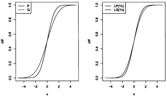
Q ao ao ci ci ao ao ci ci ~ ~ "1: "1: 0 0 N N ci ci C! 0 0 ci -4 -2 0 2 4 -4 -2 0 2 4 x x

Figure 1.3 Qualitative Robustness

In Figure 1.3, we show on the left-hand side graph two theoretical cumulative distribution functions (for two random variables P and Q) which are close. On

the right-hand side, we illustrate the empirical cumulative distribution function of the statistic Tn based on both, the distribution Fp and Fq. Since the statistic

Tn is robust, these two distributions are very close too.

This approach has many practical limitations, mainly because of its dichotomy. Thus, we need a more detailed measure which can be used in practice. In the following sections we will introduce a "quantitative" definition of robustness. 1.3 M-Estimators

M-estimators are a very general class of estimators obtained by evaluating the minimum of sums of functions of data. By Maronna et al. (2006), as special cases of M-estimators we can point out

• !east-square estimators (LSE) which are defined as the minimum of the sum of squared residuals;

• maximum likelihood estimators (MLE) which are obtained by finding the maximum of the likelihood function with respect to a (vector-valued) pa-rameter 8 on the parameter space 9.

To illustrate the concept, we consider a random sample of size n from a parametric distribution

f

8 and a maximum likelihood estimator Tn = Tn(X11 X2 , .•• , Xn)

which belongs to the class of M-estimator. The MLE is obtained by maximizing the likelihood function

n

(j

= Tn = arg max

II

hn

(Xi), TnE9 i=l

or, equivalently, by minimizing the negative log-likelihood function

n

(j

=

Tn

=

argmin

L

-ln(/Tn(Xi)). TnE9 i=l

22 The idea behind an M-estimator is to generalize this last expression to

n

Ô=

Tn

=

argmin

L

p (Xi, Tn),

Tnee i=l

where p is a function.

To formalize the concept, we consider, as in Subsection 1.2.1, two measure spaces

{x,

l:}

and {9 E

JRd, S}

where dis a positive integer and 0 E 9 is a vector of unknown parameters. An M-estimator T is defined through a measurable function

P :

x

x

e

--+

JR.

which maps a probability distribution F to the value T(F) E 9 that minimizes

1

p(x, 0) dF(x).

We assume that the function p has a derivative toP (x, 0) =

1/J

(x, 0). Thus, an M-estimator can also be defined as the solution of

(1.3.1)

i=l

or, equivalently, as the solution of

l'I/J(y,

T(G)) dG(y)

=O.

(1.3.2)

Now, we are interested in finding a general expression for the influence function of an M-estimator. Let

G

= (1 -

t)F

+

ttl.x

in Equation (1.3.2)

f

1/J

(y,

T((1- t)F

+

ttl.x)) d

((1- t)F +

ttl.x)

(y)

=

0

=>

(1- t)

f

1/J (y,

T((1-

t)F

+

ttl.x)) dF(y)

+tf

1/J (y,

T((1-

t)F

+

ttl.x)) dtl.x(Y)

= 0

=>

(1- t)

f

1/J (y,

T((1-

t)F

+

ttl.x)) dF(y)

Now we take the derivative of Equation (1.3.3) with respect to

t

and we should remember that T is a function of

t.

Therefore.

! (/

(1-

t),P(y,

T((1-

t)F

+

t~z))

dF(y)

+

t,P(x,

T((1-

t)F

+

t~z)))

=

0

=>-

J

'1/J(y,

T((1-

t)F

+

t~z))

dF(y)

(1_ ) /

(&rp(y,T((1-t)F+t~x))) (âT((1-t)F+t~z)) dF()

+

t

âT((1-

t)F

+

t~z)

EJt

Y

+

'1/J(x,

T((1-

t)F

+

t~x)

(

ô,P(x,

T((1-

t)F

+

t~x))) (âT((1-

t)F

+

t~x)) = O

+

t

âT((1-

t)F

+

t~x)

EJt

=>

J

'1/J(y,

T((1-

t)F

+

t~x))d(~x-

F)(y)

(1 _

t)

J

(&rp(y,

T((1-

t)F

+

t~x)))

(âT((1-

t)F

+

t~x)) dF( )

+

âT((1-

t)F

+

t~x)

8t

Y

(

ô,P(x,

T((1-

t)F

+

t~x))) (âT((1-

t)F

+

t~x)) = O (13 4)

+

t

âT((1-

t)F

+

t~x)

EJt ••

Now, we calculate the limit of Equation (1.3.4) when

t

--t 0

!~

(/

'1/J(y,

T((1-

t)F

+

t~x) d(~x-

F)(y)

(1 _ )

J

(&rp(y,

T((1-

t)F

+

t~x)))

(âT((1-

t)F

+

t~x)) dF( )

+

t

âT((1-

t)F

+

t~x)

EJt

Y

(

ô,P(x,

T((1-

t)F

+

t~x))) (âT((1-

t)F

+

t~x)))

+

âT((1-

t)F

+

t~x)

8t = -

J

'1/J(y,T(F)) dF(y)

+

'1/J(x, T(F)) (

âT((1-

~F

+

t~x))

lt=O

dF(y)

+

0 = 0, (1.3.5)

where we assume that the order of derivative and integration can be switched. Making use of Equation (1.2.8) and Equation (1.3.2), we obtain

'1/J(x, T(F))

+

(ô,P(y,

T{{1-

t)F

+

t~x)))

1

dF(y)

âT{{1-

t)F

+

t~x) T({l-t)F+tAz)=T(F)

24

Therefore, the influence function for a M-estimator is

IF(x;T,F)

=

'1/J(x,T(F))

.

(81/l(y,T((l-t)F+ta.,))) _{-8T((l-t)F+ta.,)} 1 _{T((l-t)F+ta.,)=T(F)}

dF( )

_y

(1.3.6)

For a maximum likelihood estimator, the '1/J function is given by

d

'1/J(x, T) =-dT

ln

Ur( x))

and let T be the maximum likelihood estimator. Then, the influence function can be written as

IF( ·TF-)=

(-~ln(fr(x)))lr-T

x, '

T { -

J

~ln

Ur(y)))

lr=T(F:f)

dFT(y)

{-1r

ln

Ur(

x)))

lr=T

(1.3.7)

To conclude this chapter, we look at sorne special cases of influence function for maximum likelihood estimators.

Example 1.4. We assume a location normal model

F(x- J.L)

= ~(x-

J.L)

where the likelihood fu.nction is

n 1

L =

I I -

exp -0.5(xi -

J.L)

2 i=l ...j2i

and the log-likelihood fu.nction is

n

l

=

L)n (

.J2i) -

0.5(xi-

J.L)

2• i=l

The derivative of the log-likelihood fu.nction with respect to the pammeter is

al n

- =

L(xi- J.L),

then we put the derivative equal to zero to find the estimator

n

L

(xi- JL)

= 0

i=l

Let 1/J(x) =x and the influence function is

x

x

1 F(x;

x,

Fx) =

f

y2 dFx(Y) =

l

=x,

sin ce

J

y2 dFx(Y)

=

J

y2 fx dy= Var(Y]- E[Y]2

=

1- 0

=

1.

Example 1.5. We assume a location logistic model

1

F(x-

JL)

= 1

+exp{

-(x-

JL)}

where the density function is

dF(x-

JL)

exp{ -(x-

JL)}

f(x-

JL)

=

d(x-

JL)

=

(1

+exp{

-(x-

JL)} )

2 •

The likelihood function is

L-

IJn

exp{

-(xi- JL)}

- i=l (1 +exp{

-(xi - JL)} )

2

and the log-likelihood function is

n

l

=

L

-(xi - JL) -

2ln(1

+

exp-(zi-1')).

i=l

26

then we put the derivative equal to zero to find the estimator

2 exp 1-0 n ( -(z;-J~) )

~

(1

+

exp-(z;-J~))

- -n =* L2F(xi- JL) -1

=

0, i=l

where there is no explicit solution for jL. Let '1/J(x)

=

2F(x) - 1 and the influence function is

I F(x;

x,

F~) ex 1/J(x).

Example 1.6. We assume a location Laplace model where the probability density functin is

f(x- JL)

=

0.5 exp{

-lx- JLI}.

The likelihood function is

n

L

=II

0.5exp{ -lxi-

JLI}

i=l

and the log-likelihood function is

n

l

=

L

-ln(2)

-lxi-

JLI

i=l

jL

=

argmin

(t

lxi-

JLI)

l=l

and

jL

=

median( x).

The derivative of log-likelihood function with respect to the parameter is

az

= {

+

1 xi

>

JL

8(x·- 11.) 1

,.- -1 Xi< JL

Therefore the influence fu.nction is

(-~ln

fT(

x))

IT-T

ex. 1/J(x)

IF( x;

x,

Fmedian(x)) =

f (

c~

..

lnfT(y))IT=T(Fi')r

dFj(Y) since the integration in denominator is a constant.

CLASSICAL MODEL FOR RESERVE IN GENERAL INSURANCE

2.1 Introduction and Motivation

In Figure 2.1, we illustrate the typical development of a daim in non-life insurance. In many cases, it is not possible for the insurer to settle a claim immediately after its occurrence. The main reasons for such a delay are:

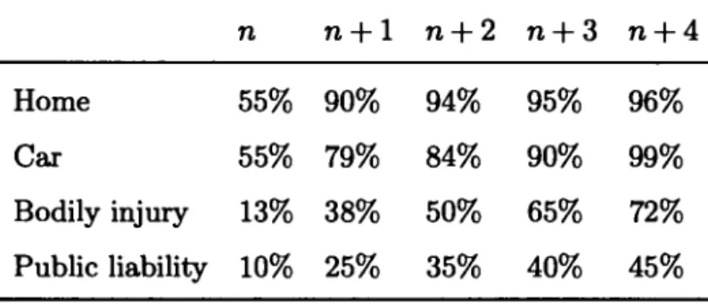
• Reporting delay: in each type of line of business there is an acceptable period in which the insured can notify the insurer of the daim occurrence. For example, in liability insurance, reporting a claim can take years. In Table 2.1, we report sorne descriptive statistics about the rate of payment in various lines of business, while n is the accident year (see Denuit et Charpentier (2004)).

• Claim verification: an insurance company may want to make ali necessary verifications about the accuracy and the authenticity of the claim. Obvi-ously, it takes sorne time before the settlement to do this process.

• Reopening of a case: in the case of gathering new information about an old case, it may be necessary to reopen the case and update the claim amount.

30

Table 2.1 Rate of payment in various lines of business.

n n+1 n+2 n+3 n+4

Home 55% 90% 94% 95% 96%

Car 55% 79% 84% 90% 99%

Bodily injury 13% 38% 50% 65% 72% Public liability 10% 25% 35% 40% 45%

order to be able to pay their future liabilities which are generated by the contracts that have been sold to the clients. This capital forms the reserve (or provision) of the non-life company. Periodically, insurance regulators require an evaluation on this reserve in order to control the financial solvency of the company and to protect policyholders. The core task of a reserving actuary is to calculate this reserve and to determine sorne characteristics of its distribution.

On the evaluation date, daims are classified in different groups according to their stage of development. These groups are illustrated on Figure 2.1. When a daim has been reported before the evaluation date but has not been completely paid, we classify the daim as reported but not settled (RBNS). When the evaluation date is after the occurrence of the daim but before the reporting date, we classify the daim as incurred but not reported (IBNR). Finally, when the evaluation date is after the occurrence date but the daim has not started to be paid, the daim is reported but not (yet) paid (RBNP). Often, this last category is grouped with the RBNS class, as illustrated on Figure 2.1. In general insurance, it is not possible to have an accurate financial condition without an accurate unpaid daim evaluation. As noted, there are sorne elements that needed to be evaluated in order to estimate the total reserve amount: a provision for RBNS daims, a provision for RBNP

31

Occurrence Payment Closing

ttTtion

_{j j j}

_j

tl

t2

t3

t4

ts

t6

~ IBNR RBNS RBNS RBNP

Figure 2.1 Claim development.

daims, a provision for IBNR daims, an estimation for reopened daim, etc. 2.2 Collective and Individual Approaches

Existing models for loss reserving can be divided into two main groups based on the granularity of the database: one can construct models for reserve by using aggregated data, i.e., data summarized by occurrence period, by development period, etc., or by using very detailed database, i.e., by using individual covariates such as information on the daim, information on the policyholder, etc.

2.2.1 Collective Approach

For nearly 40 years, the lack of detailed and accurate databases has forced the insurance companies to develop stochastic models for aggregated inform~tion.

Reserving actuaries summarize ali the information about daim payments and incurred losses in a development triangle, or run-off triangle. This structure shows the development of daims over time. It has an incrementai and a cumulative form.

32

In Table 2.2, there is a toy example of a run-off triangle for occurrence years 2010 to 2012 and annual reporting periods. A run-off triangle can be read from a variety

Table 2.2 Cumulative run-off triangle (in millions of dollars).

Accident year 12 months 24 months 36 months '2010 2011 2012 of perspectives: 100 110 120 150 160 170

• each row represents one accident year, so in our example, the fust row contains daims with occurrence year 2010, the second row contains daim payments with occurrence in 2011 and so on;

• each column represents age or maturity date: in the Table 2.2, the fust col-umn contains daims payments after 12 months, the second colcol-umn contains the cumulative daims payments after 24 months and so on; and

• each diagonal represents one calendar year. In our example, the first diag-onal (upper left corner of the triangle) is a portrait of the situation at the end of year 2010 and so on.

More formally, a collective model is constructed for a run-off triangle with occur-rence periods i

=

1, 2, ... , 1 and development periods j

=

1, 2, ... , J (without loss

of generality we assume that J = 1 in the following)

Cn

Ct(J-t) Cu C2(1-1)

where Ci; represents the total cumulative amount of claims occurred in the ith

period and paid up to period j. In order to calculate the reserve we need to predict the lower triangle in the above matrix

Cu c12 cl(J-1) Cu

c21 c22 c2(J-1)

ê21

Cat Ca2 êa(J-1)

êai

Cn ê/2 ê/(J-1)

êu

Then, the total amount of the reserve is predicted by

1 1

R

=

L

êu -

L

Ct(I-t+l)

t=l t=l

There exist similar models for incrementai run-off triangles (see Hertig (1985), Renshaw et Verrall (1998a), England et Verrall (2002), Taylor (2000)).

Collective models have been studied since the early 80s. An interested reader can consult Wüthrich et Merz (2008) for an almost complete overview. Among the collective models, the stochastic Chain-Ladder model (or Mack's model) has a special position because it produces the same reserve estimate as the Chain-Ladder algorithm and it does not make assumption about the underlying distribution of a claim amount (see Carrato et al. (1999)). Also, the mean square error of the predicted reserve amount can be calculated with an analytic formula. It will be presented in Section 2.4.

34

2.2.2 Individual Approach

For individual (or micro-level) approaches, a detailed and accurate database is essential to predict the daim development and to estimate the parameters of the model. In recent decades, the availability of detailed information on each re-ported daim and the development of strong computational tools allow creative researchers to propose individual approaches for evaluating loss reserves. Among these researchers Arjas (1989) and Norberg (1999) proposed an individual stochas-tic structure within a continuons time framework. From this base, several other models have been developed, e.g., Arjas et Haastrup (1996}, Larsen (2007}, Zhao

et

al. (2009}, Zhao et Zhou (2010) and Antonio et Plat (2014). In a discrete time

framework, Pigeon et al. (2013) and Pigeon et al. (2014) proposed an individual

model based on the Chain-Ladder structure.

This family of approaches offers a better performance when compared to collective models, allows for individual predictions and establishes a timejpayment schedule. Individual approach will not be studied in this research.

2.3 Generalized Linear Models

Generalized linear models (GLM) are a very popular class of approaches used to specify and to quantify the relation between a response variable and sorne covariates. Generalized linear models can model both individual and collective loss reserving approaches. The fust researchers who proposed loss reserving models based on generalized linear models were Renshaw et Verrall (1998a) and Renshaw et Verrall (1998b).

Generalized linear models differ from linear models in three important points:

family (since the Normal distribution is a member of this family, the linear modelisa special case of GLM but it is no longer the only option);

• the relation between the expected value of the response variable and the covariates (or independent variables) is not necessary linear: a link function describes the relation between those two components; and

• the variance of the response variable is not necessarily a constant (as in the basic linear model) and can vary according to the expected value of the dependent variable.

More details can be found in Appendix Band in McCullagh et Nelder {1989). The role of generalized linear models in general insurance is important because the Normal distribution is rarely a valid option to modelloss distributions. Moreover, the relation between the expected value of a claim and its characteristics is mostly multiplicative and hardly additive.

Definition 2.1. Let Xii' where Xii = Cii-Ci(j-1), 2 ~ j ~ I and Xil = Cil,

1 ~ i ~ I be incremental data. A generalized linear model for loss reserving is

defined by

i. incremental data Xii for different occurrence years

{i

1 =/= i2} and/ or different

development years (j1 =/=

h)

are independent;

ii. the probability density fu.nction of Xii is

where (}ii is the canonical parameter, tPii is the dispersion parameter and a() and c() are two fu.nctions.

36 Based on Definition 2.1, we obtain

E[Xïi]

=

1-'ïi

=

a'(Bïi)

Var[Xïi]

= <PïiV[xïi]

= <Pïia"(Bïi),

where <Pïi

>

0 and V[.] is a function called variance function.

The model above has 1 x J unknown parameters. They need to be estimated using information in the run-off triangle which contains less than 1 x J observations. Thus, it is inevitable to add more structure (or constraints) in the model in order to decrease the number of unknown parameters.

We assume a multiplicative structure such as

where a:i stands for the accident year effect and

tPi

stands for the development period effect. Consequently, there remain 1

+

J unknown parameters in the model: a:1, ... , a1 and

tPt, ... , tPJ·

By selecting the logarithmic link function, the model is straightforward and we ob tain

To make the model identifiable, we add an additional constraint on the model: J

L

tPi

= 1 or a:1 = 1. In the following, we choose a:1 = 1 which leads to ln (a:1) =O. j=l

Then, the number of parameters to estimate is 1

+

J - 1.

ln order to write the model in the generalized linear model framework, we group the parameters in a vector as below

and we define design matrices as

Ztj =

[o

0 0 0 0 1 0

..

·]

zij =

[o

0 1 0 0 1 0

..

·]

where 1 are in position i - 1 position 1

+

j - 1. Hence, the linear predictor of the model is

"'ii

=ln (E[Xij]) =ln

(JLii)

=

Zii/3·

(2.3.1)

Therefore the expected daim payment for cell ( i,

j)

is

E[Xij] = exp{Zij/3} = exp{ln (ai)+ ln ('1/Jj)}, where a1 = 1.

All parameters can be estimated by a maximum likelihood approach which is available in virtually all statistical software. The estimation of {3 by maximum likelihood method is

~= [Cn~

and therefore ~ evaluated by

~

=

exp{Zij~}.

In order to evaluate the risk of our reserve estimates, we need to calculate the mean square error of prediction as defined in the Theorem 2.3.1.

Theorem 2.3.1. The mean square error of prediction {MSEP) for the total paid amount

Ei êi,J

is

MSEPr:., c,J

(t

êiJ)

=

L

l/>ii

V

[Xii]

i=l i+j>l

+

_2:

38

Proof Given

the conditional mean square error of prediction (MSEP) for the total paid amount

Eiêi,J,

is

MSEPE, Cul"' (

t

êiJ)

= E [ (

t

Ô;, -

t.

C;J)

2

[V,]

= E [(

L

Xij-

L

Xij) 2 IVI] i+j>l i+j>l

=var[.~

XijiVI]

+

(.~

( x i j - E[XijiVIl) IVI)

2

•+J>l t+J>l

=Var[L Xijl

+

(L

(xij-E[XijJ))

2 ,

i+j>l i+j>l

stoc. error est. error

where for i

+

j

>

1, Xij and V1 are independent. By using the between-cell

independence, we have

MSEPE,ciJIVr

(têiJ)

=

L

Var[Xij]

+ (

L

( x i j - E[Xijl))

2

i=l i+j>l i+j>l

-

~

1

>P;; V(X;;(

+

(~,

(X;; -

E(X;;[))

2

We calculate the stochastic error and the estimation error separately and then we sum these up to obtain the ( conditional) mean square error of prediction for the total paid amount Ei

êi,J.

The difficult part is calculating the estimation error.

The unconditional MSEP is given by:

MSEPE,

c., (

t

êa)

~

E [ MSEPE, Cu IV, (

t

êu)

l

- L

r~>ijv[xïjl+E[(L

(xij-E[xïjl))

2 ]

i+j>I i+j>I

Now we fust estimate the last part

E [ ( L (xï;-E[Xïjl))

2 ]

i+j>I

L

E [(xii - E[Xïj]) (

Xmn -

E[Xmn])] i+j>I,m+n>I

{2.3.2) since Xii is not an unbiased estimator for E[Xïj] then {2.3.2) may have bias. The quadratic term in {2.3.2) will be approximated by

Var[xïi] = Var[exp{ZïJP}]

=

exp{2ZiJ,B}var[exp{Zïi,â-ZïJ.B}]

~

exp{2Zii,B}Var[zii,B]

2

[A A]

f

=

XïJZïiCov ,8,

,8

Zïi

we have used the linearization exp{z) ~ l+z for z ~ 0, in third to fourth equality. The cross term in equation {2.3.2) will be approximated by

Cov [ Xij,

X

mn]

~

exp{ Zij,B + Znmfi}Cov [ Zij,â + ZnmP]

=

XïJXnmZïiCov[,â,,â] z:nn

40

design matrix then

- (( L:

var[xi;]-

1

zi~>zi~>)

) - l i+j$1 k,l=1,2, ... ,I+J-1 =

H(p)-t.

Th en i+j>l,n+m>l 0 2.3.1 The (Over-dispersed) Poisson Model for Loss Reserving

If we choose

V[JLi;]

=

(1)JLii (recall that JLii

=

E[Xi;])

and a logarithmic link function in the generalized linear model framework ( other choices possible for the link function. Here in order to respect multiplicative affect we choose logarithmic link), we obtain a Poisson model for loss reserving. It means that incrementai payments Xii are independent random variables following Poisson distributions. Since the constraint has no effect on the total reserve amount, we can choose

J

L

1/J; =

1 or a1

=

1 and adapt the Zi; based on our choice. In the following, we

j=l

J

use

L

1/J;

= 1 to simplify the presentation. j=l

likelihood method as below:

L(x; a,

1/J,

/3)

=

II

exp{

-o:i~~~(o:i'I/Jir~:•;

i+j9 ,,.

l(x; a,

1/J,

/3)

=

L (

-o:i'I/Jj)

+xii ln

(o:i'I/Jj)

-ln (xii!) i+j9

l(x; a,

1/J,

/3)

=

L

-ez•;/3

+

Xijzii/3 -ln (xii!) i+j9

8l(x; a,

1/J,

/3) - "

(

0 0 -

z,;13)z .. -

0 1

1

J 1

8{3 - L.-! x,, e

,,t - '

t

= ' ... '

+ + '

t i+i9

(2.3.3)

where zijt is the tth element in the matrix zij and, as we saw in the previous section, ln (o:i'I/Ji) = Zii/3· The solution of the system of equations given by (2.3.3) gives us estimated values for parameters {3.

Here we calculate the MSEP for the total paid amount

Li

ciJ

with a Poisson distribution. By Theorem 2.3.1, the MSEP for a member of the exponential family is

i+j>l,n+m>l

For a Poisson random variable, we have 4>ii

=

1 and V(Xii)

=

4>iiV(xii) -V (Jl.ii) = Jl.ii. Th en

H(~)-

1

_{= ( (}

_L

_{Var [xii}

_{J -}

1

zi~>

z8>) ) -1 i+o<I _{J_ k,l=1,2, .. o,l+J-1} = ( (

L

J.t.i/

z1;>

zi~>)

) -1 i+o<I _{J_ k,l=1,2, .. o,l+J-1} Therefore

MSEPE, ciJ

(t

êiJ) =

L

Jl.ij

+

L

XijXnmZijH(~)-

1

z:nn·