HAL Id: hal-02393037
https://hal.archives-ouvertes.fr/hal-02393037
Submitted on 4 Dec 2019HAL is a multi-disciplinary open access archive for the deposit and dissemination of sci-entific research documents, whether they are pub-lished or not. The documents may come from teaching and research institutions in France or abroad, or from public or private research centers.
L’archive ouverte pluridisciplinaire HAL, est destinée au dépôt et à la diffusion de documents scientifiques de niveau recherche, publiés ou non, émanant des établissements d’enseignement et de recherche français ou étrangers, des laboratoires publics ou privés.
Assessment of physical properties of a sea dike using
multichannel analysis of surface waves and 3D forward
modeling
D. Pageot, M. Le Feuvre, D. Leparoux, P. Côté, Y. Capdeville
To cite this version:
D. Pageot, M. Le Feuvre, D. Leparoux, P. Côté, Y. Capdeville. Assessment of physical properties of a sea dike using multichannel analysis of surface waves and 3D forward modeling. Journal of Applied Geophysics, Elsevier, 2020, 172, pp.103841. �10.1016/j.jappgeo.2019.103841�. �hal-02393037�
Assessment of physical properties of a sea dike using multichannel
analysis of surface waves and 3D forward modeling
D.Pageota,*, M. Le Feuvrea, D. Leparouxa, P.Côtea, Y .Capdevilleb
a
Géophysique et Évaluation non-destructive, IFSTTAR, Bouguenais, France b
Laboratoire de Planétologie et Géodynamique de Nantes, CNRS, Université de Nantes, France
Abstract
Seismic surface waves analysis methods have been widely developed and tested in the context of subsurface characterization and have demonstrated their effectiveness for sounding and monitoring purposes. Given their efficiency, surface waves methods have been used in a variety of contexts, including civil engineering applications. However, at this particular scale, many structures exhibit 3D geometries which drastically limit the efficiency of these methods since they are mostly developed under the assumption of a semi-infinite 1D layered medium without topography. Taking advantages of wave propagation modeling algorithm development and high-performance computing center accessibility, it is now possible to consider the use of a 3D elastic forward modeling algorithm for the inversion of surface wave dispersion. We use a parallelized 3D elastic modeling code based on the spectral element method which allows to obtain accurate synthetic data with very low numerical dispersion and a reasonable numerical cost. In this study, we choose a sea dike as a case example. We first show that their longitudinal geometry and structure may have a significant effect on dispersion diagrams of Rayleigh waves. Then, we investigate the sensitivity of the dispersion diagrams to small velocity and layer thickness perturbations, and show the limitations of the standard 1D surface wave methods approach. Finally, we demonstrate in this context the benefits of using both a 3D forward modeling engine and the whole dispersion diagram, instead of the dispersion curves only.
Keywords : Controlled source seismology ; Surface waves and free oscillations ; Wave propagation ; Inversion
*Corresponding author
1. Introduction
Sea dikes are of critical importance to protect coastal areas from flooding events, but defects can form within or below the dike body, and weaken the structure (Kortenhaus et al., 2002). Following the recent storm surges in Western Europe, leading to numerous catastrophic sea dikes breaching, assessment and monitoring of sea dikes became an important task in civil engineering (Niederleithinger et al., 2012; Samyn et al., 2014; Antoine et al., 2015). However, many dikes were built, at least, several decades ago and orignal construction drawings and maintenance history may not be reliable, when they exist at all. That leads to a lack of knowledge of the internal structure and of the geotechnical parameters required to make sure of the integrity and effectiveness of the dikes. Even if the relationship between geotechnical and geophysical parameters is not straightforward, geophysicals methods are the best candidates to sound and to monitor sea dikes.
Among geophysical methods already in use for sea dike sounding, electric-resistivity imaging (ERI) is the most common one (Johansson and Dahlin, 1996; Fargier et al., 2012; Arosio et al., 2017; Weller et al., 2014). Yet, while this method is suitable to determine water content in the dike body, and to infer the nature of materials, it does not allow to assess mechanical parameters without other site-specific experiments. In the geotechnical point of view, seismic methods seem to be more adapted since the seismic wave velocities are related to geotechnical parameters such as the dynamic stiffness of the material (Karl et al., 2011). In particular, Spectral Analysis of Surface Waves, SASW (Nazarian et al., 1984) and Multichannel analysis of surface waves, MASW (Park et al., 2007), are commonly used for geotechnical investigations and have been recently used to assess mechanical properties of river dikes with symmetric geometries (Karl et al., 2011). Recently, ERI and MASW are used in combined geophysical survey of river dikes (Samyn et al., 2014; Busato et al., 2016), sometimes with the integration of geotechnical methods (Perri et al., 2014; Bièvre et al., 2017). Le Feuvre et al. (2015) develop cross-correlation-based passive MASW methods suitable for sea dike monitoring using sea waves or anthropogenic noise as continuous seismic sources to retrieve surface wave signal and produce high-quality dispersion diagrams. Planès et al. (2017) successfully test a seismic-interferometry technique on an earthen levee using retrieved impulse signal from cross-correlation of anthropogenic ambient seismic noise. Joubert et al. (2018) develop a passive monitoring method, using sea waves as seismic sources, and retrieve shear-wave velocity perturbations, related to water content in the sea dike body, with respect to a background velocity model previously inferred using effective dispersion curve inversion. The latter aims, as other monitoring methods, to detect and locate as precisely as possible the heterogeneities in the dike body to facilitate future geotechnical intervention. This need for precision can only be achieved with the use of an accurate background velocity model.
However, the inversion process of dispersion curves is widely based on 1D forward modeling algorithms with the assumption of a layered, laterally invariant, half-space models (Xia et al., 1999; Wathelet, 2005), while sea dikes present strong 3D surface variations which can limit the accuracy of the process (Wang et al., 2015; Borisov et al., 2017). Indeed, side reflections can disturb the dispersion diagram of Rayleigh waves for dikes with a width-to-height ratio lower than four (Karl et al., 2011) which can be the case for coastal sea dikes exhibiting asymmetric geometries and seafront promenade showing sometimes sub-vertical slopes. Pageot et al. (2016) have also shown that, even for sea dikes with symmetric geometries, internal structure layering can emphasize geometrical effects, and produce dispersion curves very different from the theoretical 1D case, for both the fundamental and superior modes. Consequently, a multi-modal inversion approach will also fail to infer accurate shear-wave velocity models.
Taking advantages of high-performance computing center accessibility and wave propagation modeling algorithm development, it is now possible, as recommended by Min and Kim (2006), to consider the use of a 3D elastic forward modeling as an engine for least-square minimization method, in
order to assess directly mechanical parameters, or to improve the results of 1D dispersion curves inversion. Here, we use a parallelized 3D elastic modeling code based on the spectral element method (Komatitsch and Vilotte, 1998) which allows to obtain accurate synthetic data with very low numerical dispersion and a reasonable numerical cost.
In this study, we choose simplified coastal sea dike geometries as case examples. We first show that both the shape of their cross-section, and the presence of a lateral reflector, may have a significant effect on Rayleigh waves dispersion diagrams. We demonstrate the limitations of the classical 1D inversion process and show the importance of taking into account the full dispersion diagram as an input instead of dispersion curves only. Then, we demonstrate the necessity of 3D elastic modeling as a forward problem for the inversion of dispersion diagrams.
2. Modeling surface wave dispersion in sea dikes 2.1. Multichannel analysis of surface waves
Currently, in civil engineering, Multichannel Analysis of Surface Waves, MASW, (Park et al., 1998, 1999, 2007) is a common method to obtain a dispersion diagram and the first step through the determination of the effective dispersion curve. Compared to Spectral Analysis of Surface Waves (SASW, Nazarian et al. (1984)), the main advantages of MASW are: the multichannel acquisition (efficient routine), the fast data processing, the identification of dispersion modes and the limitation of the impact of noise.
MASW is a wavefield transformation method in which data are transformed from space-time domain to, in most cases, frequency-wavenumber domain or frequency-velocity domain. Frequency-wavelength and frequency-slowness (McMechan and Yedlin, 1981) are two other way to represent surface wave dispersion. First, this transformation involves a Fourier transform of the signal. Then, the principle of MASW is to test phase propagation at a given frequency and velocity with respect to the source-receiver offset. For a given common shot gather, the dispersion diagram
D
, in the frequency-velocity domain, is calculated as:D (v ,ω)=
∑
i=1 NrS
i(
ω)e
i ω di v, (1)where
v
is the phase velocity,ω
is the angular frequency,N
r is the number of receivers andd
i is the source-receiver offset.S
i(ω) is the real to complex Fourier transform of the signal recorded at receiver
i
. Each signalS
i(ω) is phase-shifted using a test velocity
v
and the results are summed for each set of ω andv
.The effective dispersion curve (and potentially superior dispersion modes) is then extracted from the dispersion diagram using (semi-)automatic picking of the maximas. Note that a whitening of the complex signal at each frequency, as well as the normalization by frequency of the dispersion diagram, can be done to improve the visibility of the different propagation modes.
2.2. Spectral element method
For this study we need a numerical modeling method whose spatial discretization is suitable for representing complex environments, and which provides both high precision results and low numerical dispersion. Thus, we use the Spectral Element Method (SEM) for three-dimensional elastic wave propagation modeling (Komatitsch and Vilotte, 1998; Komatitsch et al., 1999, 2005; Festa and Vilotte, 2005).
SEM is a variant of the Finite Element Method (FEM) (Lysmer and Drake, 1972; Hulbert and Hughes, 1990; Tromp et al., 2008) based on a high-order piecewise polynomial approximation of the weak formulation of the wave equation, which leads to a spectral convergence ratio as the interpolation order increases. Considering near-surface experiments, one advantage of SEM is that the weak formulation naturally satisfies the free-surface condition used to simulate surface wave propagation with considerable accuracy (Komatitsch and Vilotte, 1998; Komatitsch et al., 1999, 2005). Contrary to FEM, which calls on a wide range of available element geometry (Dhatt et al., 2012), SEM is limited to quadrilateral elements in 2D and hexahedral elements in 3D. Note that although SEM with tetrahedral elements exists (Komatitsch et al. (2001)), it leads to theoretical complications. In any case, quadrangles and hexahedras are well suited for handling complex geometries and interface matching conditions (Cristini and Komatitsch, 2012).
In SEM, the wave-field is expressed in terms of high-degree Lagrange interpolants and the calculations of integrals are based on the quadrature of Gauss-Lobatto-Legendre (GLL). Each element is discretized with Lagrange polynomials of degree
n
l and containsn
l+1GLL points that form its local
mesh. This combination of high-degree Lagrange interpolants with the GLL integration leads to a perfectly diagonal mass matrix, which in turn provides a fully explicit time scheme suitable for numerical simulations on parallel computers (Komatitsch and Vilotte, 1998; Komatitsch et al., 1999).The spatial resolution of SEM is controlled by the typical size of an element (
Δ h
) and the polynomial degree in use on an element (n
l). Typically, a polynomial degreen
l=4
is optimal for seismic wave propagation modeling (Moczo et al., 2011) althoughn
l=8 remains numerically affordable in 2D.
To obtain accurate results, the required Δh
is of the order of λmin/2<Δ h<λ
min forn
l=4 and
λ
min<Δ
h<2λ
min forn
l=4, λ
min being the smallest wavelength of the waves propagated in the model. The time marching scheme is governed by the Courant-Friedrichs-Lewy (CFL) stability condition which ensures the stability of the scheme:Δ
t <C
Δ
h
c
max (2)where
C
is the Courant constant andc
max is the maximum wave velocity, typically the P-wave velocity. The Courant constantC
is determined empirically, depending on the application, and is fixed at a maximum of 0.30 for this study.In our study, the models are meshed with hexahedra (3D) using the GMSH open-source software package (Geuzaine and Remacle, 2009).
2.3. Models and acquisition
As said in the introduction section, we choose to focus on coastal sea dikes which can exhibit asymmetric geometries and strong slopes on the sea side, contrary to most of river dikes studied for example by Karl et al. (2011) and Planès et al. (2017).
The reference geometry model (Fig.1(a)) is a simplified version of the sea dike of Les
Moutiers-en-Retz (France) already studied by Le Feuvre et al. (2015) and Joubert et al. (2018). The body dike is
represented as a right-angled trapezoid along a lateral block with an infinite extent on the right side. The dike body and the lateral block are laid on a two-layered media which represents the two substratum layers. For convenience, this two layers are called the substratum and the half-space layer (bottom layer) thereafter.
This geometry is declined into a flat geometry model (Fig.1(b)) and a rough geometry model (Fig.1(c)). All materials are chosen to have a constant Poisson's ratio
η=0.25 and a constant density
ρ=2000 kg .m
−3. Models are divided into four areas of distinct shear-wave velocities, including a lateral block right next to the dike body. Shear wave velocities are set toV
S1=800 m . s
−1for the half-space layer and
V
S 2=600m. s
−1for the substratum layer. Additionally, we consider two cases for each geometry : 1) the lateral block has the same shear velocity that the dike body (
V
S 4=
V
S 3=400 m .s
−1) and 2) the lateral block has a different shear velocity (V
S3=400 m .s
−1and
V
S 4=500 m .s
−1) and acts consequently as a vertical reflector. The modeling of the sea (water layer) is not included here, since previous numerical tests showed that, in this particular context, an adjacent water layer does not have any significant effect on the dispersion diagram (Pageot et al., 2016).
Figure 2 shows the mesh corresponding to the model presents in Figure 1(a). This mesh has 11544 hexaedra elements with PML (9600 hexaedral elements without PML), the other two models have 11752 and 10712 hexaedras for the flat and the rough geometry, respectively. The lateral block always exists even when it has the same properties than the dike's body.
The linear acquisition composed of 80 receivers spaced of one meter, is placed on the crest of the sea dike body along the coast line as schematically represented on Figure 2. This study is carried out in the framework of sea dikes monitoring using ambient seismic noise. In this case, the elastodynamic Green's function of the medium can be retrieved from the cross-correlation of two recording of seismic ambient noises at different receiver location at the free surface (Wapenaar, 2004; Gouedard et al., 2008). The resulting Green's function is the wavefield that would be observed at one of these receiver positions if there were an impulsive source at the other. Taking one receiver of an array as virtual source, a complete shot gather can be retrieved and can be used to calculate a dispersion diagram using the MASW approach. Consequently, we consider a minimum source-receiver offset of one meter at the beginning of the array to act as a retrieved shot gather from ambient seismic noises. The source is a Ricker wavelet with a peak frequency of 25 Hz (
f
max≈ 70 Hz
).3. Effects of geometry and lateral reflectors
In this section, we focus on the effect of the structure of the dike, i.e. the slope angle and the presence of a lateral reflector, on dispersion diagrams. We compare calculated effective dispersion curves with theoretical ones since they are the input data in classical 1D inversion processes. The theoretical dispersion curves are calculated using a one-dimensional three-layered model corresponding to a vertical
profile going through the dike body, the substratum layer and the half-space.
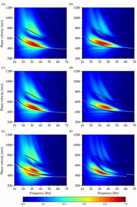
Figures 3(a-f) show the resulting dispersion diagrams for the six models considered (two different internal properties distribution and three geometries). Figure 3(a) shows that the presence of a single reflecting side (part of the free surface) does not disturb the fundamental mode compared to the 1D theoretical one. However, Figure 3(b) shows that the presence of a lateral velocity variation, even with a moderate velocity constrast with the dike's body, has effects on both the fundamental and superior modes.
We also see that contrary to the flat geometry models (Fig.3(c,d)), which has no important effects on the dispersion diagrams compared to the reference ones, the rough geometry models drastically affects the diagram. Indeed, for the first material distribution (Fig.3(e)), the fundamental mode surface wave energy appears to be split in two branches, while for the second material distribution (Fig.3(f)), the fundamental mode seems to move closer to the theoretical dispersion curve.
In Figure 3(e), the two branches would be considered as effective mode and superior mode, while they are, in reality, totally different from the theoretical one.
Note that whatever the geometry, models without lateral variation of velocity seems to strongly excited superior modes (relative to the fundamental one) around the point (
750m . s
−1; 35 Hz). We deduce here that one effect of the lateral variation of velocity is to focus energy on an effective mode and consequently to decrease the amount of energy in the superior modes.Given these results, it appears clearly that picking dispersion curves and assessing the physical properties by 1D inversion will be, on some cases, challenging. However, it is difficult, based only on the appearance of the dispersion diagram, to assess which parameter will be affected during the inversion and to what extent. In the next sections, we will focus on the reference geometry models with the lateral variation of velocity since it constitutes the closest approximation to the sea dike of Les Moutiers-en-Retz. 4. 1D inversion using particle swarm optimization
Assessing S-wave velocity model of a targeted medium by the inversion of dispersion curves is a non-linear and mix-determined problem (Socco et al., 2010). Among the methods developed and used for the inversion procedure, the least-square minimization method (Tarantola and Valette, 1982) is the most widely used. However, since this method requires an accurate initial model located in the vicinity of the global minimum of the cost function, a strong \textit{a priori} on the true model parameters is needed.
In order to avoid this issue and to start with minimum prior information, one can chose to use global optimization methods such as Monte-Carlo (Metropolis et al., 1953; Mosegaard and Tarantola, 1995; Mosegaard and Sambridge, 2002; Socco and Boiero, 2008), neighborhood algorithm (Sambridge, 1999a, 1999b, 2001; Wathelet, 2005), simulated annealing (Ryden and Park, 2006) or genetic algorithm (Holland, 1984; Dal Moro et al., 2007).
In this work, we choose to use a global optimization method called Particle Swarm Optimization (PSO). PSO, first proposed by Eberhart and Kennedy (1995), is a population-based algorithm which intends for simulating the social behavior of a bird flock (swarm of particles) to reach the optimum region of the search space.
PSO is quite recent in the framework of geophysical data inversion (Shaw and Srivastava, 2007; Yuan et al., 2009) and is not yet as widely as the other global optimization methods mentioned previously. However, it was successfully applied to surface-wave analysis (Song et al., 2012; Wilken and Rabbel, 2012), traveltime tomography (Tronicke et al., 2012; Luu et al., 2016), seismic refraction
(Poormirzaee et al., 2014), seismic wave impedance inversion in igneous rock (Yang et al., 2017) and multifrequency GPR inversion (Salucci et al., 2017). Furthermore, Song et al. (2012) have shown, in a comparative analysis, that PSO outperforms genetic algorithm and Monte-Carlo methods in terms of reliability and computational efforts. Added to this simplicity of implementation and the few number of control parameters, PSO appears as a promising method.
The standard PSO update formulas are \citep{eberhart1995new}:
v
idk +1=
v
idk+
c
1r
1(
p
id−
x
kid)+
c
2r
2(
p
gd−
x
idk)
,
(3)x
idk +1=
x
idk+
v
idk+ 1,
(4) wherer
1 andr
2 are random variables that induce stochacity (Souravlias and Parsopoulos, 2016),c
1 is the cognitive parameter,c
2 is the social parameter andc
1=
c
2=2 in most cases.
Classical improvements of PSO focus on the control of the velocity vector through the use of an inertia weight
ω
or a constriction factor κ (Shi and Eberhart, 1998; Clerc, 1999; Eberhart and Shi, 2000).v
idk +1=
ω v
idk+
c
1r
1(
p
id−
x
kid)+
c
2r
2(
p
gd−
x
idk)
,
(5)v
id k +1=κ [v
id k+
c
1r
1(
p
id−
x
idk)+
c
2r
2(
p
gd−
x
idk)]
,
(6)κ=
2
2−ϕ−
√
ϕ
2−4 ϕ
(7) where ϕ=c1+
c
2 and ϕ> 4.Here, we choose to follow the recommendations of Eberhart and Shi (2000) and to use the constrictor factor version of the algorithms and we chose
c
1=2.8 and
c
2=1.3 as recommended by Song
et al. (2012). In addition, we use the toroidal topology since it was demonstrated best performances than the initial full topology (Kennedy and Mendes, 2002).For each PSO process, we have set the swarm population to 20 particles and the number of iterations to 200. Ten processes were made for each inversion of the effective dispersion curve corresponding to the reference geometry model with lateral variation of velocity (Fig.3(b)). Two parameterizations are considered: (1) 3-layer model with variable
V
S (200<VSi<1200m / s, i=1,2,3) and
thicknessh
(1<h<10 m for the dike's body and 1<h<15 m for the substratum layer), and (2) same as (1) with a constant top layer thickness (dike's body height of 4.75 m).Figure 4 shows the results of these inversions processes for the two parametrizations. At first, we observe that for the two parameterizations, retrieved dispersion curves are in very good agreement with the input one. However, in both cases, even if the velocities of each layer are well recovered, the depth of the interface between the substratum layer and the half-space is always over-estimated. It appears also that the height of the first layer (dike body) is under-estimated (3.75 m instead of 4.75 m) with the first parametrization. Finally, it must be noted that the inversion results with a constant dike height always have higher misfit values than those obtained for a non-constant dike height.
models are not so far from the true model, does not give sufficiently accurate velocity models for geotechnical purposes.
Further, whatever the parametrization, a global optimization method can provide a set of possible solutions that are very different from each other. In this case, it can be difficult to deduce a representative average model that can be used as an initial or background model.
5. Sensitivity
In this section, we explore the effects, on dispersion diagrams, of a 10% positive perturbation of shear-wave velocity in each block constituting the reference geometry model for the second material distribution case (with a lateral variation of velocity,
V
S3=400 m/ s,
V
S 4=500 m/ s). In Figure 5 and
Figure 6, the resulting dispersion diagram of each perturbed model is compared to the original one in terms of ratio of differences (absolute value of the relative change: (x
A−
x
B)/
x
B. These results allow to determine in which frequency band the surface waves carry information about the S-wave velocity of each block.As expected, when considering only the dispersion curve, it is seen that high-frequencies carry information about the superficial layer (dike's body) and the depth of investigation increases with lower frequencies. However, Figures 5 and 6 show that information exists out of the dispersion curve domain. It is particularity significant in Figures 5(a) and Figure 5(b) where difference ratios are very important out of the dispersion curve domain. We see also ,on Figure 5(c), that the differences for a velocity perturbation of the bottom layer are weak compared to superficial layers (Fig. 5(a,b) and 6(c)) and are out of the dispersion curve domain. This means that the sensitivity of the effective dispersion curve to velocity perturbations in the bottom layer is null.
This implies that an inverted S-wave velocity models obtained using only the effective dispersion curve cannot be accurate, especially for deep layers as found in the 1D inversion results presented in the previous section. This inaccuracy can have serious implications in terms of geotechnical engineering, in particular to determine the location of the potential defects or weak zones.
These results confirm that the exploitation of the full dispersion diagram, instead of dispersion curve only, is necessary to assess correctly all parameter of interest (S-wave velocity, layer thickness). For targets with strong 3D geometry such as sea dikes, it means that the use of 3D modeling engine is necessary to provide the full dispersion diagrams needed as input during an inversion process.
In the next section, we focus on 3D inversion using the least-square minimization approach.
6. 3D inversion using the least-square minimization method
We have shown in the previous section that superior modes of dispersion diagrams carry additional information, and it is known that they allow to improve the model resolution (Gabriels et al., 1987; Park et al., 1998; Socco and Strobbia, 2004; Luo et al., 2008). However, superior modes are not always easy to identify since they can be very close to the fundamental mode over some frequency bands, or not visible at all on the dispersion diagram due to a lack of energy. Maraschini et al. (2010) have developed an efficient multi-modal inversion of surface waves, based on the module of theoretical dispersion diagram, which allows to avoid mode-misidentification errors, but the forward problem is still
1D.
Given that the differences between the true and the theoretical dispersion curves are related to the presence of a vertical reflector (lateral variation of velocity) and the footprint of the sensitivity of S-wave velocities is stronger outside the dispersion curve level, presented in the previous sections, any 1D modeling tool can encounter difficulties to retrieve accurately the velocities of a sea dike with strong 3D geometry. Consequently, we choose to use a least-square minimization method (Tarantola and Valette, 1982), based on a 3D forward modeling tool, that minimizes the misfit between the reference and calculated dispersion diagrams, instead of the dispersion curves only. This allows to avoid the dispersion curve picking step and to exploit completely the dispersion diagram. The misfit function is defined as:
C (m)=
1
2
|
d
cal(
m)−d
obs(
m)
|
2
,
where
d
cal andd
obs are, in our case, the calculated and observed dispersion diagrams, respectively. In the framework of this local optimization method, the modelm
is update iteratively through the formulation:m
k+ 1=
m
k+α Δ m ,
where
k
is the iteration number and α is scalar≤1
. The model update Δm
is deduced from:H (m
k)Δ
m
k=−∇
C(m
k)
,
where
H (m
k) is the hessian matrix and ∇
C(m
k) is the gradient vector of the cost function.
Following the Gauss-Newton approximation, Equation 10 can be rewritten as:J
T(
m
k)
J (m
k)
Δ m
k=−
J
T(
m
k)(
d
cal(
m
k)−
d
obs)
,
where
J (m)
is the Jacobian operator:J (m)=∂ d
cal/∂
m
.Given there are few unknowns (one S-wave velocity per block and the thickness of the substratum layer), the calculations of the Jacobian and the model update are very fast at each iteration.
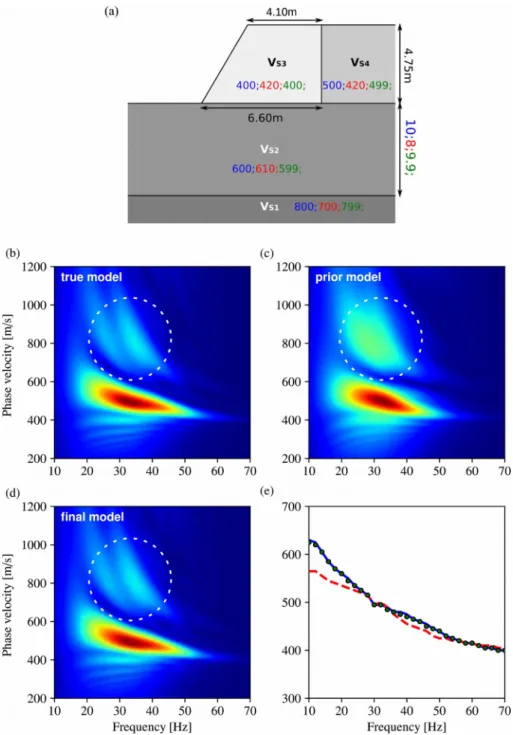
For the initial model, we use the reference geometry model with initial velocities and second layer thickness previously given by the best previous 1D inversion result (minimum misfit) obtained for a fixed dike height. We also set the initial velocity of the lateral block (
V
S 4) equal to the velocity of the dike body (V
S3). Initial velocities for each material and the initial second layer thickness are marked in blue in Fig. 7(a). For the 3D modeling, a mesh is automatically generated before each forward problem to take into account the minimum S-wave velocity of each block and the thickness of the substratum layer.Retrieved velocities using 3D least-square inversion are marked in green in Fig. 7(a). We see that all assessed velocities are almost identical to the true one (marked in blue) and more, that the inversion process allows to retrieve the velocity of the lateral block (
V
S 4). Even the thickness of the substratum layer is accurately inferred. Finally, these results show that the inversion process allows to retrieve both the fundamental (Fig.7(e)) and the superior modes (Fig.7(b), (c) and (d)) which contain additional informations on the structure and would allow for even more efficient 3D inversion from Rayleigh wave dispersion diagrams.7. Conclusions
Civil engineering structures are more and more instrumented in a sustainable way, in order to ensure the security of populations. Perturbation-based seismic methods, such as the use of ambient noises in the context of sea dikes (Le Feuvre et al., 2015; Planès et al., 2017; Joubert et al., 2018) may allow to better understand their evolution in the face of aging, by providing relative variations of the surface wave velocity as a function of time. Nevertheless, these methods require accurate reference models to start with to ensure a precise localization of heterogeneities.
We have shown here that the standard surface wave analysis workflow, which widely uses a 1D forward modeling engine and exploits only the fundamental dispersion curves, is not adapted to targets with strong 3D geometries. Even if the 1D retrieved velocity profiles are not far from the true velocity logs, they are not accurate enough for high stakes geotechnical studies such as sea dike monitoring and failure prevention.
We have proposed a new approach divided in two phases. First, a standard surface wave analysis workflow, based on particle swarm optimization, is used to obtain prior informations on the material properties. Then, the full dispersion diagram is exploited using a least-square minimization method combined with the use of a 3D forward modeling engine, in order to take into account the geometry.
This approach has shown a very good efficiency to assess physical properties of the considered sea dike, even for materials outside the vertical plan defined by the source-receivers line: the resulting model is virtually identical to the true one. An evaluation with more realistic data such as data from experimental small-scale modeling (Bretaudeau et al., 2011; Pageot et al., 2017) must be performed, but it seems at this stage that, even with field data, this method will be able to provide well defined image of the material distribution of a structure and an accurate reference model suitable for perturbation based imaging and monitoring.
Finally, the proposed method and workflow are not specific to sea dike imaging and can be easily transfered to others 3D objects such as bridges, dams, roads, rails and others infrastructures which need to be sounded and/or monitored.
8. Acknowledgments
We would like to thank the CEA for the SEM3D Spectral Element Method modeling code. We are also grateful to the CCIPL (Nantes, France) for providing access to its high-performance computing facilities and for the support given by its staff. This study was carried out within the framework of the VIBRIS project (OSUNA-IFSTTAR- University of Nantes -CNRS) and the WeaMEC PROSE project sponsored by the Region Pays-de-la-Loire (France). We would also like to thank ANR HIWAI (ANR-16-CE31-0022, Laboratory of Planetology and Geodynamics, University of Nantes, France) for its support.
Figure 1: Three sea dike geometries. (a) Reference geometry close to the real one from Les
Moutiers-en-Retz, France. (b) Flat geometry. (c) Rough geometry. The S-wave velocity of the lateral block (
V
S 4) can be equal or greater than the S-wave velocity of dike body (V
S 4).Figure 2: The mesh uses for 3D modeling (here without PML). The red dot represents the source position while the red line represents the receiver line.
Figure 3: (a,b) Dispersion diagrams for the reference geometry model (a) without lateral variation of velocity (
V
S3=
V
S4=400 m/ s) and (b) with lateral variation of velocity (
V
S3=400 m/ s,
V
S 4=500 m/ s). (c,d) Same as (a) and (b) for the flat geometry models. (e,f) Same as (a) and (b)
for the rough geometry models. Black lines correspond to theoretical fundamental and superior mode. White solid circles correspond to effective mode extracted from the dispersion diagram.Figure 4 : Results of standard 1D inversion for the reference geometry model with a lateral variation of the velocity (a,b) with a variable top layer height and (c,d) with a fixed top layer height (dike height of 4.75 m). (a, c) Dispersion curves of the best model found during inversion (grey) compared to the effective dispersion curve (black). (b,d) Best S-wave 1D velocity profiles found during inversion (grey) compared to the S-wave 1D velocity profile below the receiver line.
Figure 5: (a,c,e) Dispersion diagrams for a velocity perturbation in (a) the dike body (
V
S3), (c) the substratum layer (V
S 2) and (e) the half-space(V
S1). (b,d,f) Difference ratio between the dispersion diagram of the original model and the dispersion diagram of the perturbed models (a), (c) and (e) respectively. The red dot lines correspond to the effective dispersion curves extracted from the perturbed velocity models.Figure 6: (a) Dispersion diagrams for a velocity perturbation in the lateral block. (b) Difference ratio between the dispersion diagram of the original model and the dispersion diagram of the perturbed model (a). The red dot lines correspond to the effective dispersion curves extracted from the perturbed velocity model.
Figure 7: (a) S-wave velocity for prior model (red), inverted model (green) and true model (blue, reference geometry model with a lateral variation of velocity, Fig.1(b). (b,c,d) Dispersion diagrams for (b) the true model, (c) the prior model and (d) the inverted model.(e) Dispersion curves extracted from dispersion diagrams for the prior model (red), the inverted model (green circles) and the true model (blue). Dashed circles emphasize higher-modes.
Antoine, R., Fauchard, C., Fargier, Y., Durand, E., 2015. Detection of leakage areas in an earth embankment from GPR measurements and permeability logging. Int. J. Geophys. 2015.
Arosio, D., Munda, S., Tresoldi, G., Papini, M., Longoni, L., Zanzi, L., 2017. A customized resistivity system for monitoring saturation and seepage in earthen levees: installation and validation. Open Geosci. 9, 457–467.
Bièvre, G., Lacroix, P., Oxarango, L., Goutaland, D., Monnot, G., Fargier, Y., 2017. Integration of geotechnical and geophysical techniques for the characterization of a small earth-filled canal dyke and the localization of water leakage. J. Appl. Geophys. 139, 1–15.
Borisov, D., Modrak, R., Gao, F., Tromp, J., 2017. 3D elastic full-waveform inversion of surface waves in the presence of irregular topography using an envelope-based misfit function. Geophysics 83, R1–R11.
Bretaudeau, F., Leparoux, D., Durand, O., Abraham, O., 2011. Small-scale modeling of onshore seismic experiment: A tool to validate numerical modeling and seismic imaging methods. Geophysics 76(5), T101–T112.
Busato, L., Boaga, J., Peruzzo, L., Himi, M., Cola, S., Bersan, S., Cassiani, G., 2016. Combined geophysical surveys for the characterization of a reconstructed river embankment. Eng. Geol. 211, 74–84.
Clerc, M., 1999. The swarm and the queen: towards a deterministic and adaptive particle swarm optimization, in: Evolutionary Computation, 1999. CEC 99. Proceedings of the 1999 Congress On. pp. 1951–1957.
Cristini, P., Komatitsch, D., 2012. Some illustrative examples of the use of a spectral-element method in ocean acoustics. J. Acoust. Soc. Am. 131, 229. https://doi.org/10.1121/1.3682459
Dal Moro, G., Pipan, M., Gabrielli, P., 2007. Rayleigh wave dispersion curve inversion via genetic algorithms and Marginal Posterior Probability Density estimation. J. Appl. Geophys. 61, 39–55.
https://doi.org/10.1016/j.jappgeo.2006.04.002
Dhatt, G., Lefrançois, E., Touzot, G., 2012. Finite element method. John Wiley & Sons.
Eberhart, R., Kennedy, J., 1995. A new optimizer using particle swarm theory, in: Micro Machine and Human Science, 1995. MHS’95., Proceedings of the Sixth International Symposium On. pp. 39– 43.
Eberhart, R.C., Shi, Y., 2000. Comparing inertia weights and constriction factors in particle swarm optimization, in: Evolutionary Computation, 2000. Proceedings of the 2000 Congress On. pp. 84– 88.
Fargier, Y., Lopes, S.P., Fauchard, C., François, D., Côte, P., 2012. 2D-Electrical Resistivity Imaging for Sike Survey: Impact of the a Priori Information Management, in: Near Surface Geoscience 2012– 18th European Meeting of Environmental and Engineering Geophysics.
Festa, G., Vilotte, J.-P., 2005. The Newmark scheme as velocity–stress time-staggering: an efficient PML implementation for spectral element simulations of elastodynamics. Geophys. J. Int. 161, 789– 812. https://doi.org/10.1111/j.1365-246X.2005.02601.x
Gabriels, P., Snieder, R., Nolet, G., 1987. In situ measurements of shear-wave velocity in sediments with higher-mode Rayleigh waves. Geophys. Prospect. 35, 187–196.
Geuzaine, C., Remacle, J.-F., 2009. Gmsh: A 3-D finite element mesh generator with built-in pre-and post-processing facilities. Int. J. Numer. Methods Eng. 79, 1309–1331.
Gouedard, P., Stehly, L., Brenguier, F., Campillo, M., Colin de Verdiere, Y., Larose, E., Margerin, L., Roux, P., Sánchez-Sesma, F.J., Shapiro, N.M., others, 2008. Cross-correlation of random fields: Mathematical approach and applications. Geophys. Prospect. 56, 375–393.
Holland, J.H., 1984. Genetic algorithms and adaptation, in: Adaptive Control of Ill-Defined Systems. Springer, pp. 317–333.
Hulbert, G.M., Hughes, T.J., 1990. Space-time finite element methods for second-order hyperbolic equations. Comput. Methods Appl. Mech. Eng. 84, 327–348.
Johansson, S., Dahlin, T., 1996. Seepage monitoring in an earth embankment dam by repeated resistivity measurements. Eur. J. Eng. Environ. Geophys. 1, 229–247.
Joubert, A., Le Feuvre, M., Côte, P., 2018. Passive monitoring of a sea dike during a tidal cycle using sea waves as a seismic noise source. Geophys. J. Int. 214, 1364–1378.
Karl, L., Fechner, T., Schevenels, M., François, S., Degrande, G., 2011. Geotechnical characterization of a river dyke by surface waves. Surf. Geophys. 9, 515–527.
Kennedy, J., Mendes, R., 2002. Population structure and particle swarm performance, in: Evolutionary Computation, 2002. CEC’02. Proceedings of the 2002 Congress On. pp. 1671–1676.
Komatitsch, D., Martin, R., Tromp, J., Taylor, M.A., Wingate, B.A., 2001. Wave propagation in 2-D elastic media using a spectral element method with triangles and quadrangles. J. Comput. Acoust. 9, 703–718.
Komatitsch, D., Tsuboi, S., Tromp, J., 2005. The spectral-element method in seismology. Seism. Earth Array Anal. Broadband Seism. 205–227.
Komatitsch, D., Vilotte, J.-P., 1998. The spectral element method: An efficient tool to simulate the seismic response of 2D and 3D geological structures. Bull. Seismol. Soc. Am. 88, 368–392. Komatitsch, D., Vilotte, J.-P., Vai, R., Castillo-Covarrubias, J.M., Sanchez-Sesma, F.J., 1999. The
spectral element method for elastic wave equations-application to 2-D and 3-D seismic problems. Int. J. Numer. Methods Eng. 45, 1139–1164.
Kortenhaus, A., Oumeraci, H., Weissman, R., Richwien, W., 2002. Failure mode and fault tree analysis for sea and estuary dikes, in: Coastal Engineering Conference. pp. 2386–2398.
Le Feuvre, M., Joubert, A., Leparoux, D., Côte, P., 2015. Passive multi-channel analysis of surface waves with cross-correlations and beamforming. Application to a sea dike. J. Appl. Geophys. 114, 36–
51.
Luo, Y., Xu, Y., Liu, Q., Xia, J., 2008. Rayleigh-wave dispersive energy imaging and mode separating by high-resolution linear Radon transform. Lead. Edge 27, 1536–1542.
Luu, K., Noble, M., Gesret, A., 2016. A competitive particle swarm optimization for nonlinear first arrival traveltime tomography, in: SEG Technical Program Expanded Abstracts 2016. Society of Exploration Geophysicists, pp. 2740–2744.
Lysmer, J., Drake, L.A., 1972. A finite element method for seismology. Methods Comput. Phys. 11, 181– 216.
Maraschini, M., Ernst, F., Foti, S., Socco, L.V., 2010. A new misfit function for multimodal inversion of surface waves. Geophysics 75, 31.
McMechan, G.A., Yedlin, M.J., 1981. Analysis of dispersive waves by wave field transformation. Geophysics 46, 869–874.
Metropolis, N., Rosenbluth, A.W., Rosenbluth, M.N., Teller, A.H., Teller, E., 1953. Equation of state calculations by fast computing machines. J. Chem. Phys. 21, 1087–1092.
Min, D.-J., Kim, H.-S., 2006. Feasibility of the surface-wave method for the assessment of physical properties of a dam using numerical analysis. J. Appl. Geophys. 59, 236–243.
Moczo, P., Kristek, J., Galis, M., Chaljub, E., Etienne, V., 2011. 3-D finite-difference, finite-element, discontinuous-Galerkin and spectral-element schemes analysed for their accuracy with respect to P-wave to S-wave speed ratio. Geophys. J. Int. 187, 1645–1667.
Mosegaard, K., Sambridge, M., 2002. Monte Carlo analysis of inverse problems. Inverse Probl. 18, 29. Mosegaard, K., Tarantola, A., 1995. Monte Carlo sampling of solutions to inverse problems. J. Geophys.
Res. Solid Earth 100, 12431–12447.
Nazarian, S., Stokoe, I.I., Kenneth, H., 1984. Nondestructive testing of pavements using surface waves. Niederleithinger, E., Weller, A., Lewis, R., 2012. Evaluation of geophysical techniques for dike
inspection. J. Environ. Eng. Geophys. 17, 185–195.
Pageot, D., Le Feuvre, M., Donatienne, L., Philippe, C., Yann, C., 2016. Importance of a 3D forward modeling tool for surface wave analysis methods, in: EGU General Assembly Conference Abstracts. p. 11812.
Pageot, D., Leparoux, D., Le Feuvre, M., Durand, O., Côte, P., Capdeville, Y., 2017. Improving the seismic small-scale modelling by comparison with numerical methods. Geophys. J. Int. 211, 637– 649. https://doi.org/10.1093/gji/ggx309
Park, C.B., Miller, R.D., Xia, J., 1999. Multichannel analysis of surface waves. Geophysics 64, 800–808. Park, C.B., Miller, R.D., Xia, J., Ivanov, J., 2007. Multichannel analysis of surface waves (MASW)—
active and passive methods. Lead. Edge 26, 60–64.
multi-channel record, in: SEG Expanded Abstracts. pp. 1377–1380.
Perri, M.T., Boaga, J., Bersan, S., Cassiani, G., Cola, S., Deiana, R., Simonini, P., Patti, S., 2014. River embankment characterization: The joint use of geophysical and geotechnical techniques. J. Appl. Geophys. 110, 5–22.
Planès, T., Rittgers, J.B., Mooney, M.A., Kanning, W., Draganov, D., 2017. Monitoring the tidal response of a sea levee with ambient seismic noise. J. Appl. Geophys. 138, 255–263.
Poormirzaee, R., Moghadam, R.H., Zarean, A., 2014. Introducing Particle Swarm Optimization (PSO) to Invert Refraction Seismic Data, in: Near Surface Geoscience 2014-20th European Meeting of Environmental and Engineering Geophysics.
Ryden, N., Park, C.B., 2006. Fast simulated annealing inversion of surface waves on pavement using phase-velocity spectra. Geophysics 71, 49.
Salucci, M., Poli, L., Anselmi, N., Massa, A., 2017. Multifrequency Particle Swarm Optimization for Enhanced Multiresolution GPR Microwave Imaging. IEEE Trans. Geosci. Remote Sens. 55, 1305–1317.
Sambridge, M., 2001. Finding acceptable models in nonlinear inverse problems using a neighbourhood algorithm. Inverse Probl. 17, 387.
Sambridge, M., 1999a. Geophysical inversion with a neighbourhood algorithm—I. Searching a parameter space. Geophys. J. Int. 138, 479–494. https://doi.org/10.1046/j.1365-246X.1999.00876.x
Sambridge, M., 1999b. Geophysical inversion with a neighbourhood algorithm—II. Appraising the ensemble. Geophys. J. Int. 138, 727–746.
Samyn, K., Mathieu, F., Bitri, A., Nachbaur, A., Closset, L., 2014. Integrated geophysical approach in assessing karst presence and sinkhole susceptibility along flood-protection dykes of the Loire River, Orléans, France. Eng. Geol. 183, 170–184.
Shaw, R., Srivastava, S., 2007. Particle swarm optimization: A new tool to invert geophysical data. Geophysics 72, 75.
Shi, Y., Eberhart, R., 1998. A modified particle swarm optimizer, in: Evolutionary Computation Proceedings, 1998. IEEE World Congress on Computational Intelligence., The 1998 IEEE International Conference On. pp. 69–73.
Socco, L.V., Boiero, D., 2008. Improved Monte Carlo inversion of surface wave data. Geophys. Prospect. 56, 357–371.
Socco, L.V., Foti, S., Boiero, D., 2010. Surface-wave analysis for building near-surface velocity models —Established approaches and new perspectives. Geophysics 75, 75–83.
Socco, L.V., Strobbia, C., 2004. Surface-wave method for near-surface characterization: a tutorial. Surf. Geophys. 2, 165–185.
Song, X., Tang, L., Lv, X., Fang, H., Gu, H., 2012. Application of particle swarm optimization to interpret Rayleigh wave dispersion curves. J. Appl. Geophys. 84, 1–13.
https://doi.org/10.1016/j.jappgeo.2012.05.011
Souravlias, D., Parsopoulos, K.E., 2016. Particle swarm optimization with neighborhood-based budget allocation. Int. J. Mach. Learn. Cybern. 7, 451–477.
Tarantola, A., Valette, B., 1982. Generalized nonlinear inverse problems solved using the least squares criterion. Rev. Geophys. 20, 219–232.
Tromp, J., Komattisch, D., Liu, Q., 2008. Spectral-element and adjoint methods in seismology. Commun. Comput. Phys. 3, 1–32.
Tronicke, J., Paasche, H., Böniger, U., 2012. Crosshole traveltime tomography using particle swarm optimization: A near-surface field example. Geophysics 77, 19.
Wang, L., Xu, Y., Xia, J., Luo, Y., 2015. Effect of near-surface topography on high-frequency Rayleigh-wave propagation. J. Appl. Geophys. 116, 93–103.
Wapenaar, K., 2004. Retrieving the elastodynamic Green’s function of an arbitrary inhomogeneous medium by cross correlation. Phys. Rev. Lett. 93, 254301.
Wathelet, M., 2005. Array recrecord of ambient vibrations: surface-wave inversion (PhD Thesis). Université de Liège.
Weller, A., Lewis, R., Canh, T., Möller, M., Scholz, B., 2014. Geotechnical and geophysical long-term monitoring at a levee of Red River in Vietnam. J. Environ. Eng. Geophys. 19, 183–192.
Wilken, D., Rabbel, W., 2012. On the application of Particle Swarm Optimization strategies on Scholte-wave inversion. Geophys. J. Int. 190, 580–594. https://doi.org/10.1111/j.1365-246X.2012.05500.x
Xia, J., Miller, R.D., Park, C.B., 1999. Estimation of near-surface shear-wave velocity by inversion of Rayleigh waves. Geophysics 64, 691–700.
Yang, H., Xu, Y., Peng, G., Yu, G., Chen, M., Duan, W., Zhu, Y., Cui, Y., Wang, X., 2017. Particle swarm optimization and its application to seismic inversion of igneous rocks. Int. J. Min. Sci. Technol. 27, 349–357.
Yuan, S., Wang, S., Tian, N., 2009. Swarm intelligence optimization and its application in geophysical data inversion. Appl. Geophys. 6, 166–174. https://doi.org/10.1007/s11770-009-0018-x


![[PDF] Introduction à la Conception Objet et à C++ pdf | Cours informatique](data:image/gif;base64,R0lGODlhAQABAIAAAP///wAAACH5BAEAAAAALAAAAAABAAEAAAICRAEAOw==)