HAL Id: hal-01180818
https://hal.archives-ouvertes.fr/hal-01180818
Submitted on 4 Nov 2015
HAL is a multi-disciplinary open access archive for the deposit and dissemination of sci-entific research documents, whether they are pub-lished or not. The documents may come from teaching and research institutions in France or abroad, or from public or private research centers.
L’archive ouverte pluridisciplinaire HAL, est destinée au dépôt et à la diffusion de documents scientifiques de niveau recherche, publiés ou non, émanant des établissements d’enseignement et de recherche français ou étrangers, des laboratoires publics ou privés.
Distributed under a Creative Commons Attribution - NonCommercial - ShareAlike| 4.0
Bayesian and Hybrid Cramér–Rao Bounds for the
Carrier Recovery Under Dynamic Phase Uncertain
Channels
Jianxiao Yang, Benoit Geller, Stéphanie Bay
To cite this version:
Jianxiao Yang, Benoit Geller, Stéphanie Bay. Bayesian and Hybrid Cramér–Rao Bounds for the Carrier Recovery Under Dynamic Phase Uncertain Channels. IEEE Transactions on Signal Processing, Institute of Electrical and Electronics Engineers, 2011, pp.667-680. �10.1109/TSP.2010.2081981�. �hal-01180818�
Abstract—In this paper, we study Bayesian and hybrid Cramér-Rao bounds (BCRB and HCRB) for the code-aided (CA), the
data-aided (DA) and the non-data-aided (NDA) dynamical phase estimation of QAM modulated signals. We address the bounds derivation for both the off-line scenario, for which the whole observation frame is used, and the on-line which only takes into account the current and the previous observations. For the CA scenario we show that the computation of the Bayesian information matrix (BIM) and of the hybrid information matrix (HIM) is NP hard. We then resort to the belief-propagation (BP) algorithm or to the Bahl-Cocke-Jelinek-Raviv (BCJR) algorithm to obtain some approximate values. Moreover, in order to avoid the calculus of the inverse of the BIM and of the HIM, we present some closed form expressions for the various CRBs, which greatly reduces the computation complexity. Finally, some simulations allow us to compare the possible improvements enabled by the off-line and the CA scenarios.
Index Terms—Bayesian Cramér-Rao Bound (BCRB), Code-Aided (CA) Bound, Data-Aided (DA) Bound, Dynamical Phase
Estimation, Hybrid Cramér-Rao Bound (HCRB), Non-Data-Aided (NDA), On-line, Off-line
I. INTRODUCTION
S well-known, optimal estimators cannot always be built in practical implementations. Assessing the achievable estimation performance may be difficult, and one often has to resort to simulations and then compare the performance to some lower bounds corresponding to the optimum performance. Lower bounds give an indication of the performance limitations, and consequently, they can also be used to determine whether some imposed performance requirements are realistic or not. Although there exists many lower bounds, the Cramér-Rao bounds (CRB) are the most commonly used [1]-[3] because they achieve a good
1
This work was partially funded by the ANR LURGA program and was presented in part at ICC 2009.
Jianxiao Yang and Benoît Geller are with UEI ENSTA, ParisTech, 32 Boulevard Victor, 75015 Paris, France (e-mail: [email protected] and [email protected]);
Jianxiao Yang, Benoît Geller, and Stephanie Bay1
Bayesian and Hybrid Cramér-Rao Bounds for
the Carrier Recovery under Dynamic Phase
Uncertain Channels
accuracy at the price of a reasonable computation difficulty.
There are three ways to use data in a telecommunication system [4]: data aided (DA), code aided (CA) and non data aided (NDA) estimations. Earlier attempts of signal synchronization in the low-SNR regime focused either on the so-called data-aided (DA) or non-data-aided (NDA) synchronization mode [5], [6]. On the one hand, DA parameter estimation techniques rely on the presence of pilot symbols in the data frame and may lead to unacceptable losses in terms of power and spectral efficiency. On the other hand, NDA synchronization algorithms drop some statistical information about the transmitted data and may lead to very poor results at low SNR. As a consequence, it was recognized [7],[8] that the only way to achieve a good performance compromise both in terms of acquisition time and steady-state accuracy (the so-called jitter variance) is to take advantage of the coding gain not only for data detection, but also for synchronization as well. This led to the notion of code aided (CA) synchronization, i.e., explicitly using the channel code structure and properties to perform a satisfying synchronization without any known pilot.
Many works concern the Cramér-Rao bounds for the carrier phase and frequency estimation. Most of them are related to constant (i.e., non-dynamic) carrier phase and frequency. For instance the CRB for phase and /or frequency estimation with known data has been derived in [9]-[11]. Some phase and frequency CRBs for DA and NDA PSK or QAM signals have been derived in [12]-[18]. In particular some analytical expressions of those CRBs at low SNR have been derived in [19],[20]. For PSK signals, the CRBs for DA and NDA estimators were computed in [21],[22] for both the case of phase estimation and the case of joint phase and frequency estimation. Still for the static carrier phase, the CA standard CRB (SCRB) has been derived in [23]-[25] using the first derivative of the log-likelihood function expressed in terms of the marginal a posteriori probabilities (APPs) of the coded symbols. One of the most important contributions of these papers is the application of the BCJR algorithm [37] to the APP computation which was first applied to calculate the APPs of the convolutional code (CC) aided SCRB [23] and was then extended to the evaluation of the APPs of turbo code (TC) aided SCRB in [24]. Moreover, the CA CRBs for joint static parameters estimation problem (carrier phase, carrier frequency and timing estimation) was achieved with the use of the BCJR algorithm in [25].
However, in modern high rate communication systems, one cannot rely on a constant phase model and must take into account time-varying phase noise due to the oscillator instabilities [26]-[33]. To quantify the resulting performance degradation, [26] considered the data aided CRB for the frequency offset estimation with a phase noise variance. [31] has derived a Bayesian CRB (BCRB) for the NDA BPSK signal with dynamical phase offset. When a deterministic parameter (such as a linear drift) is jointly to be considered, the hybrid CRB (HCRB) is relevant; the HCRB was applied to the case of the dynamical phase estimation as briefly sketched in [32] for NDA BPSK signal and in [33] for coded QAM signals. The goal and the contribution of this paper is to give both the BCRB and the HCRB for the dynamical time-varying phase estimation in the case of QAM modulated signals and for the different scenarios (NDA, CA and DA). We present some closed form expressions for the various CRBs based on the second derivatives of the log-likelihood function; by detailing the derivations, we show that the exact calculation of the HCRB is
theoretically NP hard and cannot be easily calculated (the SCRB is just a special case of the HCRB). The obtained closed form expressions give a clearer insight of the corresponding information matrix elements and this enables us to justify some simplifications. Moreover, we display how the different bounds for the deterministic and stochastic parameters of interest behave in the different scenarios (off-line / on-line, DA / CA / NDA) and we give asymptotic results. Note that similarly to [31],[32] which provide a satisfying benchmark for the non coded BPSK phase estimation algorithm [34], these derived CRBs provide very good benchmarks for the more difficult QAM phase estimation algorithms both in NDA [35] and CA [36] scenarios.
This paper is thus organized as follows. In section II, we recall the various kinds of Cramér-Rao bounds. After describing the system model in section III, we derive the Bayesian and the hybrid Cramér-Rao bounds for off-line estimations for the DA, CA and NDA scenarios in section IV. The on-line bound is derived in section V and the different results are illustrated and interpreted in the final section.2
II. CRAMÉR-RAO BOUNDS REVIEW
Different kinds of CRBs can be considered. In the following, we briefly describe the links between on one side the HCRB, and on the other side the standard CRB and the BCRB.
We consider the most general case including both deterministic and random parameters for hybrid estimation. Denote this parameter vector asu
u uTr, Td
T , where ud is assumed to be a
nm
1 deterministic vector and ur is assumed to be a m1random vector with an a priori probability density function (pdf)p u
r . The true value of ud is denotedud. We consider ˆu y
asan estimator of uwhere y is the observation vector. The HCRB satisfies the following inequality on the MSE
1
,r|d d ˆ ˆ |d d T d Ey u uu u y u u y u uu H u , (1)where H u
d is the so-called hybrid information matrix (HIM) and is defined as
d E,r|d d logp
, r| d
|dd
u
y u u u u u u
H u y u u . (2)
It is shown in [32] that inequality (1) is still respected when the deterministic and the random parts of the parameter vector are dependent. Byexpanding the log-likelihoodaslogp
y u, r|ud
lnp
y u u| r, d
lnp
ur|ud
, the HIM can be rewritten as2
The notational convention adopted is as follows: italic indicates a scalar quantity, as in a ; boldface indicates a vector quantity, as in a and capital boldface indicates a matrix quantity as inA. The ( , )th
m n entry of matrix A is denoted as Am n, . The transpose matrix of A is indicated by a superscript
T
A , and A is the determinant ofA. n
m
a represents the vectoram, ,anT, where m and nare positive integers (mn). Re a and Im a are respectively the real and imaginary parts of a. Exy denotes the expectation over x and y. u and
v
u represent the first and second order derivative operators. Finally, a is designated as the value taken by variable a.
d Er|dd
d, r
Er|dd lnp
r| d
d d
u
u u u u u u u u u
H u F u u u u , (3)
where F u u
d, r
is the Fisher information matrix (FIM) [2] defined by
d, r
|r,d d ln
| d, r
|d dE p
u
y u u u u u u
F u u y u u . (4)
In (3), the Fisher information matrix F u u
d, r
gives the contribution of the observations whereas the second term on the rightside corresponds to the contribution of the a priori distribution. It is then straightforward to re-obtain the standard and the Bayesian CRBs as particular cases. If uud, thenHreduces to
| ln
|
| d d d d d d d d E p d u y u u u u u H u F u y u , (5)and the inverse of (5) is just the standard CRB [1]. If uur, we have that
rln
r r r r r E E p u u u u H F u u , (6) where
| ln
|
r r r r E p r u y u u F u y u (7)and the inverse of H in (6) is the Bayesian CRB [2].
Because (5)-(6) can be considered as special cases of the general definition given in (3), in section IV, we first give the detailed derivation of the HCRB for the QAM dynamical phase estimation and it is then easy to obtain the BCRB for our problem.
III. SYSTEM MODEL
We consider the transmission over an additive white Gaussian noise (AWGN) channel of a modulated sequence
1, ,
T Ls s
s ,
where the symbols sl belong to a constellation set SM
s1, ,sM
(M-QAM, M-PSK or M-APSK), affected by some carrier phaseoffsets stacked in a vector
1, ,
T L
θ . Assuming that the timing recovery is perfect and that there is no inter-symbol interference
(ISI), the sampled baseband signal
1, ,
T L y y y is written as
l l j j l l l l l l y s e n a jb e n, (8) where sl, l and nl are respectively theth
l transmitted complex symbol (sl al jbl with E s
l 0 and
2 1 2 2 l M l l s s E s s M
Sis the transmitted signal power), the residual phase distortion that must be eliminated and the zero mean circular Gaussian noise with known variance 2
n
For the data-aided (DA) system, the transmitted symbols are known. As the observations and the transmitted symbols are independent and the additive noise is Gaussian distributed, the conditional probability based on the known phase θ is
2 2 2 2
2
1 1 Re 1 | exp exp 2 l L j L L l l l l l l l n l n n y s e s y p p y
y | θ . (9)For the non-data-aided (NDA) system, the transmitted symbols are independent and identically distributed (i.i.d.). Hence the conditional probability based on the known phase θ is
2 2 2 2
2
1 1 2 Re 1 1 | exp exp l l M L j L L l l l l l l l n l s n n y s e s y p p y M
S y | θ . (10)For the code-aided (CA) system, the independent and identically distributed (i.i.d.) condition between the transmitted symbols does not hold any more, instead the i.i.d. condition holds between the codewords. A message of Kbits is encoded into a N bit codeword
1, ,2 ,
| 1, ,2
K
N v
c c c v
c c which is then in practice further mapped as a symbol vector s c
v
s1
cv , ,sL
cv
.Hence, the conditional probability based on the known phase vector θ is
2 2 1 1 2 2 2 2 2 2 1 1 | | , | , Re 1 1 exp exp 2 . 2 K K K l v v v v v v L L j l l v l v l K v l n n n p p p p p y s e s y
y θ y c c θ c c y s s c θ s s c c c (11)We now consider the phase model. In practice, there is a constant frequency shift between the transmitter’s clock and the receiver’s clock. The corresponding phase distortion is linear. Furthermore, clocks are never perfect and oscillators suffer from jitters. This results in a Brownian phase model with a linear drift
1
l l wl
, (12) where l is the unknown phase offset at time l, is the unknown constant frequency offset (linear drift), wl is a white Gaussian
noise with zero mean and variance 2 w
. This model is commonly used [26]-[34] in order to describe the behavior of practical oscillators for which the frequency is randomly perturbed. The corresponding conditional probability can be expressed as
1
2 1 2 1 | , exp 2 2 l l l l w w p . (13)Note that from (12), the joint pdf p
θ|
can be written as
1
1
2 | | , L l l l p p p
θ . (14)IV. CRBS FOR THE DYNAMICAL PHASE ESTIMATION
In practical receivers, phase estimation can actually be considered following two main scenarios: off-line and on-line. With off-line synchronization, the carrier phase offset θ is not estimated until the whole observation frame y has been received. In the rest of this section, we derive some analytical expressions for bounds corresponding to the off-line carrier phase offsets estimation. In a subsequent paragraph, these expressions will further allow us to find some bounds for the on-line scenario.
The parameters of the phase model (12) include some random parameters
1, ,
T L
θ (i.e. the dynamical phase) and a
deterministic parameter (i.e. the scalar linear drift), so that the parameter vector can be written as
r d u θ u u . (15)
Equation (3) thus becomes
|
|
|
| | | , | | | | | | ln | , ln | , ln | ln | ln | , ln | , ln | ln | , T T p p p p E E E p p p p E θ ξ θ θ θ θ θ θ y θ ξ ξ θ θ ξ θ θ y θ y θ ξ θ ξ θ H y θ ξ y θ ξ θ θ F
| | | | | ln | ln | ln | T ln | p p E p p θ θ θ θ θ θ ξ θ θ θ θ . (16) where
| | | , | | ln | , ln | , , ln | , T ln | , p p E p p θ ξ θ θ y θ ξ ξ θ ξ y θ y θ ξ F θ y θ ξ y θ ξ .We then decompose the hybrid information matrix (HIM) H into a block matrix that will be useful in the sequel
11 12 11 12 21 22 12 22 T H H H H H H H H H , (17) where
11 , | | | | 12 , | | | | 21 22 , | | | | ln | , ln | ln | , ln | ln | , ln | . T E p E p E p E p E p E p θ θ θ θ y θ θ ξ ξ θ θ y θ θ ξ ξ ξ ξ y θ θ H y θ ξ θ ξ H y θ ξ θ ξ H H y θ ξ θ ξ . (18)From (8)-(11), one can see that the log likelihood function lnp
y θ| ,
does not depend on ; consequently, the partial derivatives ξθlogp
y θ ξ| ,
|ξ ξ and ξξlogp
y θ ξ| ,
|ξ ξ are both equal to zero. The hybrid block matrix can thus be written as:
| | 1 | , | | | 1 | | | | | | | ln | ln | ln | , ln | ln | 0 ln | ln | ln | L T L p p E p E E p p p p E E p θ θ θ θ θ y θ θ θ θ θ θ θ θ θ θ θ ξ θ y θ 0 H θ θ 0 θ ξ θ F θ θ
ln
|
| T p θ , (19)where
| ,
| 1 1 ln | , 0 L L E p θ θ y θ y θ 0 F θ 0 and
11 | | , | | | 12 | | 21 22 | | ln | , ln | ln | ln | . T E E p E p E p E p θ θ θ θ θ y θ θ ξ θ θ ξ ξ θ H y θ θ ξ H θ ξ H H θ ξ . (20)First, the DA and NDA scenarios are briefly reviewed in sections IV.A and IV.B, as a simplified version has already been presented in [33]. Then the more difficult to tackle CA scenario is detailed in section IV.C.
A. Computation of Eθ| F
,θ for the DA scenarioThe evaluation of the term Eθ| F
,θ requires the computation of the FIM F
,θ , which in turn requires the evaluation ofthe Hessian of the log-likelihood functionlnp
y θ| ,
. For both the DA and NDA scenarios, according to the observation model defined previously, after a marginalization on the independent symbols, and then using both the independence of the transmitted symbols and the whiteness of the noise, one finds that:
1 1 ln | , ln | , , ln | l L L l l l l l l l s l p p y s p s p y θθ y θ θθ
θθ
. (21)One can realize that each term of the sum (21) is a matrix with only one non-zero element at most, namely,
,
lnp | , l l lnp yl|l
θθ y θ θθ . (22)
As a direct consequence, the Hessian θθlnp
y θ| ,
is a diagonal matrix with the lth diagonal element given by (22). Moreover,because of the circularity of the observation noise, the expectation of (22) with respect to p y
l|l
does not depend onl.Discarding the last zero line and column, one then obtains
| D L,
Eθ F θJ I (23) where IL is the L L identity matrix and JD is defined as follows
2 , | 2 ln | , . D l p J E y θ y θ (24)Starting from (9) with the DA scenario where p y
l| l,
p y
l| l, ,sl
and taking the first and the second derivatives, one easilyobtains that
2 2 Im ln | , ln | , , jl l l l l l l l n y s e p p y s y θ (25)and
2 2 2 2 2 2Re ln | , ln | , , jl l l l l l l l n y s e p p y s y θ . (26)So in the DA case, (24) becomes
DA 2
2 2 2 ln | , 2 2 SNR s D l n p J E y,θ y θ , (27)where the signal-to-noise ratio is defined as 2 2 SNR s n.
B. Computation of Eθ|F
,θ for the NDA scenarioWe now turn to the NDA scenario. With an appropriate marginalization on the transmitted symbols, we obtain by deriving (10)
ln
| , ,
ln | ln | , ln | , . l M l l l s l l l l l l p y s p p p y
S y θ y θ (28)As the derivation is a linear operator, we find that
| , , | , , | , , ln | , | , , | , , | , l M l M l M l M l M l l l l l l l l l s s l s l l l l l l l l l l l s s p y s p y s p y s p p y s p y s p y
S S S S S y θ (29) Moreover as
ln | , , 1 | , , | , , l l l l l l l l l l l p y s p y s p y s , using (25) we have
2 2 Im | , , | , , l j l l l l l l l l l n y s e p y s p y s . Consequently we obtain
2 2 Im ln | , Pr | , , , l l M j l l l l l s l n y s e p s y
S y θ (30) where Pr
| , ,
| , ,
| , l l l l l l l l l p y s p s s y p y is the marginalized a posteriori probability (APP) of sl based on the observation yl
with known phase.
Taking the second derivative of lnp
y θ| ,
, using (25), (26), (30) and following a similar calculus, we further find that
2 2 2 2 2 2 2 2 2 2 ln | , ln | , | , , | , , | , , | , , 2 Im 2 Re Pr | , , l M l M l M l M l l l l l l l l l l l l s l s l l l l l l l s s j j l l l l l l l n n p p y p y s p y s p y s p y s y s e y s e s y
S S S S y θ
2 2 2 Im Pr | , , . l l M l M j l l l l l s s n y s e s y
S S (31)In general, the expectation of (31) with respect to Pr
sl|yl, , l
does not have any simple analytical solution. Hence, in practice, we have to evaluate NDA 2
| 2 ln | , D l p J E y,θ y θ (32) by numerical integration.C. Computation of Eθ|F
,θ for the CA scenarioFor the CA scenario, because of the code structure, the independence condition between symbols does not hold anymore. Using (11), one has that
2
2
1 1 1 ln | , ln | , , ln | , , K K L v v l l l v l v v v l p p p p y s s p
y θ y c c θ c c c c c . (33)From (70)-(72) in the Appendix, we show that the first and the second derivatives can respectively be expressed as
2
1 ln | , , ln | , Pr | , , K m m m v m v v m m p y s s p
c y θ c c y θ , (34) for mn
2 2 1 ln | , , ln | , , ln | , ln | , ln | , Pr | , , K m m m v m n n n v n v v m n m n m n p y s s p y s s p p p
c c y θ y θ y θ c c y θ , (35) and for mn
2
2
2 2 2 2 2 1 ln | , , ln | , , ln | , ln | , Pr | , , K m m m v m m m m v m v v m m m m p y s s p y s s p p
c c y θ y θ c c y θ . (36)All these derivatives are too hard to use in practice because they all involve an exponential number of sums. We thus propose the following method to find a good approximation of these derivatives. From (34), the first derivative can be further expressed as follows
2 2 1 1 2 1 1 ln | , , ln | , , ln | , Pr | , , Pr , | , , ln | , , Pr , | , , , K K K v m m m v m m m m v m v v m m v v v m m m M m m i m v m m v m i v i m y s s p y s s p s s p y s s s s s s
c c c c y θ c c y θ c c c y θ c c c y θ (37) where
1, if 0, otherwise. v m i m i s s s s c c (38) Thus
2 1 1 2 1 ln | , ln | , , Pr , , | , , 2 Im Pr | , , , K m M m m i m v m m v m i i v m m j M m i m i i n p p y s s s s s s y s e s s
y θ c c c y θ y θ (39) where
2
2
1 1 Pr | , , Pr , , | , , Pr , | , , K K v m i v m m v m i v m m v m i v v s s s s s s s s s s y θ
cc c y θ
cc c y θ c c . (40)The term Pr
smsi| , ,y θ
in (39) is exactly the a posteriori probability of the code aided scenario.Similarly to the first derivative (39), the second derivatives (35) for nm can be further expressed as
1 1 2 2 2 1 2 1 ln | , , ln | , , ln | , ln | , ln | , Pr , , | , , ln | , Pr , , , , | , , K K m m m v m n n n v n v m m v n n v v n m m n m n m m i v m m v m i n n v n i v p y s s p y s s p p p s s s s p y s s s s s s s s s s
c c y θ y θ y θ c c c c y θ c c c c y θ
2 1 2 1 2 1 2 1 2 1 1 2 2 1 1 , ln | , , ln | , ln | , 2Im 2Im ln | , ln | , Pr , | , , , m n M M m n n i n i i m n m n j j M M m i n i m i n i i i n n m n p y s s p p y s e y s e p p s s s s
y θ y θ y θ y θ y θ (41) where
1 2 1 2 1 2 2 1 2 1 Pr , | , , Pr , , , , | , , Pr , , | , , . K K v v m i n i v m m v m i n n v n i v v m m v n n v m i n i v s s s s s s s s s s s s s s s s s s s s
c c c c y θ c c c c y θ c c c c y θ (42)Like the term Pr
smsi| , ,y θ
in (39), the term Pr
sms si1, nsi2| , ,y θ
in (41) is also an a posteriori probability of the codeaided scenario and it measures the dependency between the symbols in position n and in position m. Actually the evaluation of
2 ln | , n m p y θin (41) for any couple of positions really burdens the computation complexity. If the codeword has been sufficiently
interleaved, the term Pr
sms si1, nsi2| , ,y θ
can be approximately expressed as the product of two independent probabilities, i.e.
1 2
1
2
Pr sms si, nsi | , ,y θ Pr smsi | , ,y θ Pr snsi | , ,y θ . We can then further simplify (41) as
1 2 1 2 1 2 1 2 1 1 2 2 2 1 1 2 2 1 2 Im 2 Im ln | , ln | , ln | , Pr | , , Pr | , , 2 Im 2 Im Pr | , , Pr m n m n j j M M m i n i m i n i i i n m n n m n j j M m i n i m i n i i n n y s e y s e p p p s s s s y s e y s e s s s s
y θ y θ y θ y θ y θ r θ
2
2 0 ln | , ln | , | , , 0, M i m n p p
y θ y θ r θ (43)where the last equality comes from (39).
2 2 2 2 2 2 2 1 1 2 2 ln | , ln | , , ln | , , ln | , Pr , , | , , ln | , , ln | , , Pr | , , M m m i m m m i m v m m v m i i v m m m m m m i m m m i m m i m m p p y s s p y s s p s s s s p y s s p y s s s s
y θ y θ c c c y θ y θ
2 2 1 2 2 2 2 2 1 1 1 ln | , 2 Re 2 Im 2 Im Pr | , , Pr | , , Pr | , , . m m m M i m j j j M M M m i m i m i m i m i m i i n i n i n p y s e y s e y s e s s s s s s
y θ y θ y θ y θ (44)We thus obtain the expression of the second derivatives as follows when the code has been sufficiently interleaved
2 2 2 4 2 2 1 1 0, ln | , 4 Im 2 Re 2 Im = Pr | , , Pr | , , , m m m j j j M M m i m i m i n m m i m i i n n i n n m p y s e y s e y s e s s s s n m
y θ y θ y θ (45)Actually, the calculation of Pr
smsi| , ,y θ
is also NP hard (see (40)) and theoretically requires 2 Ksums. In practice we just have to resort to some classical a posteriori probability (APP) decoding algorithms, namely the famous Bahl-Cocke-Jelinek-Raviv (BCJR) algorithm [37] or the belief propagation (BP) algorithm [38]-[40], in order to calculate the approximate value of
Pr smsi| , ,y θ . In the rest of the paper, we assume that the code has been sufficiently interleaved so that (45) holds.Moreover,
discarding the last zero line and column, the FIM then has an identity matrix form as
CAD L
EθF θ J I , (46) where IL is the L L identity matrix and
CA 2
| 2 ln | , D l p J E y,θ y θcan be obtained from (45) with a Monte Carlo
simulation.
D. Computation of the HIM
As mentioned in (17), the HIM can be divided into four submatrices; due to the model of Section III, assuming that we have no a priori knowledge on the initial phase, one obtains that the upper left part H11, which corresponds to the random parameters θ, has
a particular mathematical structure just like in [31]
11 1, 1 0 0 1 1 0 0 0 0 1 1 0 0 1 1 A A b A A H , (47) where 2 2 2 1 . w D w A J b (48)
2 2 12 21 1 , 1 2, 1 T T w L w H H 0 , (49)
2 22 L1 w. H (50)E. The Bayesian Cramér-Rao bounds (BCRBs)
When there is no linear drift, the parameter vector ucontains only random parameters θ, i.e. uurθ. In this scenario, the
BCRB is the lower bound of the MSE. Moreover, the Bayesian information matrix (BIM) BL is equal to the upper left sub-matrix
of the HIM, i.e.
11
L
B H . (51) The diagonal element 1
, L l l
B of the inverse of matrix BL is the off-line BCRB associated to the estimation ofl. Furthermore,
the corresponding analytical expression associated with the off-line BCRB has already been obtained in Appendix I. D of [31]
2 2 1
1 1 2 3 2 3 2 2 1 1 2 11 , , 1 1 1 2 2 2 1 2 1 2 1 2 L L L L l L l L L l l l l L b r r b r r b r r r r A H B B , (52) where
1 2 2 1 1 2 2 2 1 1 1 4 2, 1 1 1 4 2, w D w D w D w D r J J r J J (53) and
1 1 1 2 2 2 1 1 1 1 2 2 2 2 1 4 1 2 2 1 4 , 1 4 1 2 2 1 4 . D w D w D w D w D w D w J J J J J J (54)F. The hybrid Cramér-Rao bounds (HCRBs)
We nowinverse the HIM to obtain the analytical expression of the HCRB. In the sequel, we shall need the expression of the elements of the first row of 1
11
H . We proceed similarly as in [32]. From (47), thanks to the cofactor expression of the matrix inversion formula we have
1 1 11 1, 1 11 l L l L l l b d bd H H , (55)1 0 0 1 1 0 0 0 0 1 1 0 0 1 l A A D b A A , (56)
and dl satisfies the following recursive equation
2
1 2,
l l l
d Abd b d with d01 and d1bA. (57)
Similarly to Appendix I.A of [31], dl can thus be rewritten as 1 1 2 2
l l
l
d r r , where r1,r2,1 and 2 were given in (53) and
(54). We then obtain from (55)
1 1 1 1 11 1, 1 1 1 2 2 2 11 l L l L l l b r r b r r b H H . (58)Thanks to the block-matrix inversion formula [3], we now can find the expression of the inverse of the HIM
1 1 1 1 11 11 12 1 1 1 12 11 L T H V H H H H H , (59) where 1 12 11 12 2 1 T w L H H H , (60) and 1 1 1 11 12 12 11 T L V H H H H . (61)
We start to compute corresponding to the inverse of the minimum bound on.Dueto the particular structures of matrices H11
and H12 (see (47),(49)), we get
1 1
11 11 2 4 1,1 1, 1 2 L w w L H H , (62) where 1 11 1,1 H and 1 11 1, L H are given by (58).We now derive an analytical expression for the diagonal elements of the upper left part
1
11 L
H V corresponding to the
minimum bound onθ (see (59)). From the definition ofVLin (61), the diagonal elements
VL l l, can be written as
2
2 1 1 1 1 11 11 11 11 4 4 , 1, , 1, 1, 1 1 1 L l l l L l l L l w w V H H H H . (63)Inserting (58) into (63) and then into (59), we obtain the analytical expression of the upper diagonal elements 1 , l l
H i.e. the
2 2 1 1 2 3 2 3 2 2 1 1 2 1 1 1 2 2 2 1 2 1 2 , 11 2 2 1 1 1 2 2 1 1 1 2 2 2 1 1 1 2 2 2 2 11 1 2 . L L L L l L l L l l l L l L l L l l l b r r b r r b r r r r A b b r b r r b r b r b r r b r H H H (64)Comparing to (52), we notice that the contribution of VL in (64) is the additional uncertainty brought by the linear drift .
G. High SNR Asymptote Bound
In the high-SNR range, there exists one constellation point max m
s for the NDA case (resp. max i
s for the CA case) which has a dominant a posteriori probability. Substituting
max
Pr sm |ym, m, 1 into (31) (resp.
maxPr smsl | , ,y θ 1 into (45)), the second
order derivatives can be respectively expressed as
max 2 2 2 max 2 2 Re , NDA, ln | , 2 Re , CA. m m j m m n j m m i n y s e p y s e y θ (65)Thus both NDA and CA scenarios are equivalent to the DA scenario at high SNR and one has
NDA CA DA 2 2 2 2 SNR s Dh Dh D n J J J . (66)
We thus obtain the same result as in [31]; by introducing this value into the mathematical expression of the bound, we obtain similarly to section V of [31], an asymptotic bound which is under the bound itself. Note that a far more complex expression for
NDA
Dl
J can be obtained at low SNR, and one can combine the low and high SNR HCRB asymptotes to lead to an asymptotic lower bound without any Monte-Carlo simulation.
V. ON-LINE BOUNDS
Up to this section, we have focused on the off-line scenario. We now show how the previous results can be directly used in the case of an on-line synchronization mode. In this mode, only the past and the current observations are available, i.e. 1
1, ,
T l l y y y
where lL. Like in section III of [31], the on-line BCRB (resp. HCRB) associated to vector 1 L
y is equal to entry
L L,
of the inverse of the BIM (resp. HIM); one thus readily obtains the analytical expression of the on-line BCRB (from (52)) and on-line HCRB (from (64)) associated to the estimation of l (l3)
2 2 3 2 2 3 2 2 1 1 2 1
1 1 1 2 2 2 1 2 1 2 1 2 , l l l l l l CB br r br r b rr r r A B (67)
2 2 1 2 3 2 3 2 2 1 1 2 1 1 1 2 2 2 1 2 1 2 11 2 2 1 1 1 2 2 1 1 1 2 2 2 1 1 1 2 2 2 2 11 1 and 2 , l l l l l l l l C b r r b r r b r r r r A l b b r b r r b r r b r r b r l H H H (68)wherer1,r2,1and 2 are given by (53),(54), and H11
l is a l l matrix with the same form as H11of equation (47).VI. DISCUSSION
We now display simulation results with Gray mapping QAM symbols for different scenarios. For the code aided scenario, we use a recursive systematic rate 1 2 turbo code (mother code rate 1 3) whose generator polynomials are G137OCT and G221OCT
with a S random interleaver [41]. Since turbo code can be described by means of a trellis, the marginal APPs can be efficiently computed by the famous BCJR algorithm [37].
-5 0 5 10 15 20 25 30 -38.4 -38.2 -38 -37.8 -37.6 -37.4 -37.2 -37 -36.8 -36.6 SNR (dB) M S E ( d B ) HCRB ( = 0.03rad, w2 = 0.01rad2 ) NDA, 256QAM, L = 72 NDA, 64QAM, L = 72 NDA, 16QAM, L = 72 NDA, QPSK, L = 72 NDA, BPSK, L = 72 DA, L = 72 -5 0 5 10 15 20 -38.5 -38 -37.5 -37 -36.5 -36 -35.5 SNR (dB) M S E ( d B ) HCRB ( = 0.03rad, w 2 = 0.01rad2 ) CA, 256QAM, L = 72 CA, 64QAM, L = 72 CA, 16QAM, L = 72 CA, QPSK, L = 72 CA, BPSK, L = 72 DA, L = 72
Fig. 1 NDA (left), CA (right) and DA HCRB for different constellations as a function of the SNR
We start with figure 1 displaying the behavior of the HCRB on as a function of the SNR; we compare the performance of NDA (on the left), CA (on the right) and DA scenarios for various constellations. At high SNR, we first see that HCRB converges to its horizontal asymptote ( 2
1
w L
) for here a symbol block length L72. The observation noise has then no influence on the estimation of the linear drift and clearly, for a larger block length or a smaller phase noise, the asymptote would be lower. Then at median SNR, HCRBleaves its asymptote and this happens at a larger SNR if a larger constellation is used. Note that the CA scenario allows to have better performance that the NDA aided scenario.
0 50 100 150 200 250 -14 -12 -10 -8 -6 -4 -2 0 2
Temporal Position in Block
M S E ( d B ) QPSK, BCRB ( = 0rad, w 2 = 0.01rad2, SNR = 0 dB ) On-Line NDA On-Line CA On-Line DA Off-Line NDA Off-Line CA Off-Line DA 50 100 150 200 250 -14 -12 -10 -8 -6 -4 -2 0 2 4 6
Temporal Position in Block
M S E ( d B ) QPSK, HCRB ( = 0.03rad, w 2 = 0.01rad2, SNR = 0 dB ) On-Line NDA On-Line CA On-Line DA Off-Line NDA Off-Line CA Off-Line DA
Fig. 2 QPSK CRB curves for the various block positions when the SNR = 0 dB
In figure 2, we now turn to the behavior of the dynamic phase bound and display some results for QPSK modulated signals as a function of the position in the block (L288). We first remark that in all the cases (BCRB/HCRB and DA/CA/NDA), the off-line scenario always gives a better result that the corresponding on-line result. To be more precise, the on-line curves always benefit from more and more observations until they saturate; at the last position the on-line bound corresponds exactly to the off-line bound. Contrarily to the on-line scenario, for the off-line scenario the best phase estimate is achieved at midblock, whereas they become poorer at the block border. This comes from the fact in the center position of the phase vector, one has more adjacent (past or future) and strongly correlated variables (see the phase model of (12)) than at the border of the block. Also logically, the DA scenario achieves a better performance than the CA aided scenario and even more than the NDA scenario. The BCRB provides the lower bound for this general block-phase estimation framework with a known linear drift (or0), whereas the HCRB provides the lower bound with an unknown linear drift. The HCRB is always lower bounded by the BCRB for any position in the block but for such a block length, there is almost no loss of information due to the linear drift for the off-line case in the center position so that the HCRB almost corresponds to the BCRB.
Instead of looking at the different positions for a given SNR, we now display HCRB curves as function of the SNR for the phase at the central position of the block. Figure 3 displays results for the BPSK modulated signal. For codes that are described by means of a trellis, the marginal symbol APPs in (40) and (42) can be approximately computed from the trellis state APPs and state transition APPs, which in turn can be determined efficiently by the famous BCJR algorithm. Like already observed on figure 2, one can see on figure 3 that the off-line scenario allows better results than the on-line scenario and also that the NDA case is worse compared to the CA and to the DA cases. Here, it is important to note that one can expect a better performance with the NDA
-8 -6 -4 -2 0 2 4 6 -18 -16 -14 -12 -10 -8 -6 -4 -2 SNR (dB) M S E ( d B ) BPSK, HCRB ( = 0.03rad, w 2 = 0.01rad2 ) NDA On-Line, L = 6912 CA On-Line ( r = 1/2 ), L = 6912 DA On-Line, L = 6912 NDA Off-Line, L = 6912 CA Off-Line ( r = 1/2 ), L = 6912 DA Off-Line, L = 6912 -8 -6 -4 -2 0 2 4 6 -10 -8 -6 -4 -2 0 2 4 6 8 SNR (dB) 1 0 *l o g 1 0 (J D ) BPSK NDA, L = 6912 CA ( r = 1/2 ), L = 6912 DA, L = 6912
Fig. 3 BPSK NDA, turbo-CA and DA HCRB curves (left) and corresponding JD (right) as functions of the SNR
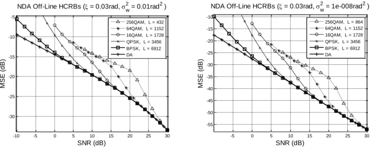
off-line scenario rather than with the CA on-line scenario. Stated in other words, in general, one can expect more benefits from the estimation method (off-line/on-line) rather than the way of using data (DA, CA or NDA). This can also be observed for other modulations and other coding schemes (e.g. simple convolutional codes) and this is a general tendency; however the results are not always totally so simple as displayed in the following figure 4 with a 16QAM modulation and some additional parameters must be taken into account.