Official URL
https://www.collegepublications.co.uk/ifcolog/?00036
Any correspondence concerning this service should be sent to the repository administrator: [email protected]
This is an author’s version published in: http://oatao.univ-toulouse.fr/22274
Open Archive Toulouse Archive Ouverte
OATAO is an open access repository that collects the work of Toulouse researchers and makes it freely available over the web where possible
To cite this version: Balbiani, Philippe and Dieguez, Martin and Fariñas del Cerro, Luis Setting the basis for Here and There modal logic. (2019) Journal of Applied Logics: The IfCoLog Journal of Logics and their Applications, 6 (7). 1475-1500. ISSN 2631-9810
S
ETTING THE
B
ASIS FOR
H
ERE AND
T
HERE
M
ODAL
L
OGICS
PHILIPPEBALBIANI
Institut de recherche en informatique de Toulouse. Toulouse University [email protected]
MARTÍN DIÉGUEZ
Centre international de mathématiques et d’informatique. Toulouse University [email protected]
LUISFARIÑAS DEL CERRO
Institut de recherche en informatique de Toulouse. Toulouse University [email protected]
Abstract
We define and study a new modal extension of the logic of Here and There with operators from modal logic K. We provide a complete axiomatisation together with several results such as the non-interdefinability of modal operators, the Hennessy-Milner and the finite model properties, a bound for the complexity of the related satisfiability problem and a discussion about the canonicity of some well-known Sahlqvist formulas in our setting. We also consider the equilibrium property on this logic and we prove the theorem of strong equivalence in the resulting framework.
1
Introduction
Modal extensions of intuitionistic logic have been studied in different domains such as philo-sophical and formal logic [6, 8, 32, 17, 39, 28, 31, 14, 42] or computer science [15, 30, 36]. Recently, combinations of intermediate and modal logics have become very interesting due to their use in the definition of nonmonotonic formalims [33, 34]. These new contributions consist in modal extensions of Here and There [26] (HT), also known as Gödel G3 [24] or Smetanich [40] logics.
Two significant works on this topic are the temporal [11] and epistemic [16] extensions of HT. The former approach extends HT with operators from Linear Time Temporal Logic [37]
(LTL) while the latter consist of an orthogonal combination of HT and the modal logic S5. Those are specific combinations of modal frames: in the former case models are as in LTL (i.e. linear frames) but every Kripke world behaves as in HT. In case of S5 models are equivalence relations where every Kripke point is regarded as a HT system. Such extensions allow extending Pearce’s Equilibrium Logic [33, 34] in a natural way.
However, the lack of a general theory supporting such extensions caught our attention. In this paper, we try to fill this gap by proposing a general methodology to define Here and There modal logics that allow extending Equilibrium Logic with modal operators. In our case, more precisely, we consider the combination of propositional HT and the modal logic
K (denoted by KHT ), where we provide detailed investigation on interdefinability of modal
operators, axiomatisation and complexity of the satisfiability problem. Moreover, we also consider the canonicity problem in the new here and there setting. On KHT , we define the concept of modal equilibrium model (the modal extension of equilibrium models) and we study several interesting properties, such as the property of strong equivalence, which can serve as a starting point for future modal extensions. The main contribution of this paper is to pave the way for the definition of tree-like extensions of Equilibrium Logic such as Propositional Dynamic[25] or Computational Tree [13] Equilibrium Logic, which have not been considered in the literature.
Since our contribution is strongly connected with previous work in the literature on Intuitionistic Modal Logic, we summarise the different approaches proposed in the literature. The first one was published by Fitch [20] who axiomatise a first-order intuitionistic version of the logic T . As stated by Simpson [39], “from a modern viewpoint, the choice of axioms seems rather arbitrary”. They are also remarkable Prior’s intuitionistic S5 modal logic (named MIP Q) [32] and Prawitz’s intuitionistic S4 [38].
The most popular approach was presented by Fischer Servi [17, 18, 19] (FS), who proposed a framework to determine the correct intuitionistic logic of a classical modal logic based on birelational models1. The same semantics were discovered independently by
Plotkin and Stirling [36]. Our decision of building our proposal based on FS is due to the fact that other existent extensions of Here and There [2] are strongly connected with FS (note that the axiomatic system proposed in [2] extends FS with some extra axioms such as, among others, Hosoi’s [27]).
However, Servi’s semantic framework is not the only one that has been considered. All differ from each other although they preserve some similarities. Among others, Boži´c and Došen [6] and Wijesekera [41] proposed a birelational approach but they differ in the interaction between the partial order and the modal accessibility relation.
When interpreting the ✷ modality, Wijesekera forces the necessity operator to be
inter-1Birelational models are Kripke models containing two accessibility relations: a partial order to interpret the
preted with respect to both relations in an attempt to imitate the behaviour of the universal quantifier of first-order intuitionistic logic. Instead, Boži´c and Došen force the models to satisfy an extra confluence property involving both accessibility relations. As a consequence, regarding the ✸-free fragment, both systems induce the same intuitionistic modal logic. When adding the ✸ modality, both systems become different. Wijesekera’s system, which interprets ✸ with respect to both accessibility relations, has some strange properties (see [39, page 48]). For instance, the addition of the schema p ∨ ¬p is not sufficient to make Wije-sekera’s logic to collapse to its classical counterpart. Moreover, it is easy to see that the axiom schema ✸ (p ∨ q) → (✸p ∨ ✸q), which is valid in FS, is not in Wijesekera’s system. Boži´c and Došen interpret ✸ only with respect to the accessibility relation for the modal connectives. Under this interpretation, the resulting logic does not satisfy the disjunction property and the modal operators are not semantically independent (i. e. the schemas ✸p ∨ ¬✷p and ✸p ↔ ¬✷¬p are valid).
Layout This paper is organised as follows. In Section 2 we present syntax and two equiva-lent alternative semantics based on Kripke models. The former semantics (the “Here and There” semantics) is simulated by two valuation functions while the latter semantics pos-sesses two accessibility relations to interpret implication and modal operators. In Sections 3 and 4, we present a sound and complete axiomatisation of this logic with respect to the birela-tional semantics. In Section 5 we discuss about the canonicity of some well-known Sahlqvist formulas in our setting. Section 6 defines bisimulations for our KHT -modal extensions and we use them to prove the non-interdefinability of modal operators and the Hennessy-Milner property in our framework. Section 7 defines the concept of modal equilibrium logic and shows that such definition is suitable for proving the theorem of strong-equivalence. We finish the paper with conclusions and future work.
2
Syntax and semantics
In this section we present the language of KHT , which coincides with the ordinary language of modal logic, and two alternative and equivalent semantics. The former is inspired by the semantics proposed in [11], while the latter is adapted from the semantics of intuitionistic modal logic described in [17, 39].
2.1 Syntax
Let V AR be a countable set of propositional variables (with typical members denoted p, q, etc). The set F OR of all formulas (with typical members denoted ϕ, ψ, etc) is defined as
follows:
ϕ:= p | ⊥ | (ϕ ∧ ψ) | (ϕ ∨ ψ) | (ϕ → ψ) | ✷ϕ | ✸ϕ. (1) As in intuitionistic logic, negation is defined in terms of implication (ϕ → ⊥). We will follow the standard rules for omission of the parentheses. Let |ϕ| denote the number of symbols in ϕ. The modal degree of a formula ϕ (in symbols deg(ϕ)) is defined as follows:
deg(ϕ) def= 0 if ϕ= p (p ∈ V AR) or ϕ = ⊥;
max(deg(ψ), deg(χ)) if ϕ= ψ ⊙ χ, with ⊙ ∈ {∧, ∨, →};
1 + deg(ψ) if ϕ= ⊙ψ, with ⊙ ∈ {✷, ✸}.
Given a nonempty set Γ of formulas, let deg(Γ) be a maximal element in {deg(ϕ) : ϕ ∈ Γ} when this set is bounded, and ω otherwise.
A theory is a (possibly infinite) set of formulas. A theory Σ is closed if it is closed under subformulas and for all formulas ϕ, if ϕ ∈ Σ then ¬ϕ ∈ Σ. For all theories x, let ✷xdef= {ϕ | ✷ϕ ∈ x} and ✸xdef= {✸ϕ | ϕ ∈ x}.
2.2 KHT semantics
An KHT -frame is a structure F = éW, Rê where: 1) W is a nonempty set of worlds;
2) R is a binary relation on W .
The size of F is the cardinal of W . Given a nonempty set W and H, T : W → 2V AR, we
say that H is included in T (in symbols H ≤ T ) if for all x ∈ W , H(x) ⊆ T (x). We write
H < T when H ≤ T and H(x) Ó= T (x) for some x ∈ W . An KHT -model is a structure M = éW, R, H, T ê where:
1) éW, Rê is an KHT -frame;
2) H, T : W → 2V AR are such that H ≤ T .
Given an KHT -model M = éW, R, H, T ê, x ∈ W , and α ∈ {h, t}, the satisfaction relation of a formula ϕ at (x, α) (in symbols M, (x, α) |= ϕ) is defined as follows:
• M, (x, h) |= p if p ∈ H (x); M, (x, t) |= p if p ∈ T (x); • M, (x, α) Ó|= ⊥;
• M, (x, α) |= ϕ ∨ ψ if M, (x, α) |= ϕ or M, (x, α) |= ψ;
• M, (x, α) |= ϕ → ψ if for all α′ ∈ {α, t} M, (x, α′) Ó|= ϕ or M, (x, α′) |= ψ; • M, (x, α) |= ✷ϕ if for all y ∈ W , if xR y then M, (y, α) |= ϕ;
• M, (x, α) |= ✸ϕ if there exists y ∈ W such that xR y and M, (y, α) |= ϕ.
Given a set Σ of formulas, we write M, (x, α) |= Σ if for all formulas ϕ ∈ Σ, M, (x, α) |=
ϕ.
The following lemma shows that the KHT semantics satisfy the persistence property of Intuitionistic Logic.
Lemma 1. Let M = éW, R, H, T ê and M′ = éW, R, T, T ê be two KHT models and let M′′ = éW, R, T ê be a K model. For all x ∈ W and for all formula ϕ,
1) IfM, (x, h) |= ϕ then M, (x, t) |= ϕ; 2) M, (x, t) |= ϕ iff M′,(x, h) |= ϕ; 3) M′,(x, h) |= ϕ iff M′′, x|= ϕ (in K).
Proof. By induction on ϕ. Left to the reader.
From the 1st item of Lemma 1, we conclude that a formula ϕ is KHT -satisfiable iff the set of all total KHT -models of ϕ is nonempty. Hence, since the set of all K-models of ϕ corresponds to the set of all KHT -models of ϕ, ϕ is KHT -satisfiable iff ϕ is K-satisfiable. Moreover, K has the finite model property and K-satisfiability is PSPACE-complete [4,
Chapter 6]. Consequently, KHT has the finite model property and KHT -satisfiability is PSPACE-complete.
Given two sets of formulas Σ and Γ, we say that Γ is a local KHT semantic consequence of Σ (denoted by Σ |= Γ) if for all KHT models M = éW, ≤, R, V ê and for all (w, α) ∈
W × {h, t} , if M, (w, α) |= Σ then M, (w, α) |= Γ. Note that, when restricting the
language to the propositional connectives, the resulting logic collapses to propositional Here and There. Therefore KHT is a conservative extension of Here and There. The following results can be proved as in Intuitionistic Modal Logic.
Lemma 2. Let M = éW, R , H, T ê be an KHT -model. For all x ∈ W and for all formulas
ϕ, M, (x, t) |= ϕ ∨ ¬ϕ.
Lemma 3. Let M = éW, R, H, T ê be an KHT -model. For all x ∈ W and for all formulas
Let ≃ be the equivalence relation between formulas defined as follows: ϕ ≃ ψ if for all
KHT -models M = éW, R, H, T ê and for all x ∈ W , M, (x, h) |= ϕ iff M, (x, h) |= ψ.As
in Intuitionistic Logic, for all formulas ϕ, ¬¬¬ϕ ≃ ¬ϕ. Hence, by a straightforward induction on the structure of a formula, we obtain the following result.
Lemma 4. Letϕ be a formula. The least closed set of formulas containing ϕ contains at
most3|ϕ| equivalence classes of formulas modulo ≃. 2.3 Birelational semantics
A birelational frame [39] is a structure F = éW, ≤, R ê where 1) W is a nonempty set of worlds;
2) ≤ is a partial order on W ; 3) R is a binary relation on W .
The size of F is the cardinal of W . F is said to be normal if it satisfies the following conditions for all x, y, z ∈ W :
1) if x ≤ y and x ≤ z then either x = y or x = z or y = z;
2) if xR y and x ≤ z then there exists t ∈ W such that y ≤ t and zR t; 3) if xR y and y ≤ z then there exists t ∈ W such that x ≤ t and tR z; 4) if x ≤ y and yR z then there exist t ∈ W such that xR t and t ≤ z.
If F is normal then for all x ∈ W , either x is a maximal element with respect to ≤, or there exists exactly one y ∈ W such that x ≤ y and x Ó= y. In the former case letxâdenote x.
In the latter case, letx denote this y. From this definition, it follows that for all x, yâ ∈ W ,
x≤ y iff either y = x, or y =x. F is said to be strongly normal if F is normal and for allâ
x, y ∈ W :
5) ifxRy then yâ =y;â
A birelational model is a structure M = éW, ≤, R , V ê where 1) éW, ≤, R ê is a birelational frame;
2) V : W → 2V AR is such that for all x, y ∈ W if x ≤ y then V (x) ⊆ V (y).
Given a birelational model M = éW, ≤, R, V ê and x ∈ W , the satisfaction relation of a formula ϕ at x in M (in symbols M, x |= ϕ) x is defined as follows:
1. M, x |= p if p ∈ V (x); 2. M, x Ó|= ⊥;
3. M, x |= ϕ ∧ ψ if M, x |= ϕ and M, x |= ψ; 4. M, x |= ϕ ∨ ψ if M, x |= ϕ or M, x |= ψ;
5. M, x |= ϕ → ψ if for all y ∈ W if x ≤ y then either M, y Ó|= ϕ or M, y |= ψ; 6. M, x |= ✷ϕ if for all y, z ∈ W , if x ≤ y and yR z then M, z |= ϕ;
7. M, x |= ✸ϕ if there exists y ∈ W such that xR y and M, y |= ϕ.
Note that the satisfaction of ✷ϕ and ✸ϕ are not symmetrical. Such asymmetry also occurs in Intuitionistic Modal Logic: while the satisfaction of the ✷ modality is accepted to be defined in terms of ≤ and R to preserve the monotonicity property, the satisfaction of ✸ is more controversial and several semantics have been discussed in the literature (as discussed in the introduction). One of the most accepted ones does not involve the ≤ relation in order to follow Kripke’s spirit of keeping the satisfaction of the eventually modality locally. Given two sets of formulas x and y, we say that y is a local KHT birelational semantic consequence of x (denoted by x |= y) if for all KHT birelational models M = éW, ≤, R, V ê and for all
w∈ W , if M, w |= x then M, w |= y.
Lemma 5. Let M = éW, ≤, R, V ê be a birelational model. If M is normal then for all
x, y ∈ W , if xRy thenxRâ y.â
Proof. Suppose that M is normal. Let x, y ∈ W be such that xRy. We know that x ≤ x.â
Since xRy, there exists z ∈ W such thatxRzâ and y ≤ z. By definition ofyâ, either z = y orâ
z ≤y. In the former case, sinceâ xRz, we conclude thatâ xRâ y. In the latter case, sinceâ xRz,â
there exists t ∈ W such thatxâ ≤ t and tRy. By definition ofâ x,â xâ= t. Thus,xRâ y.â 2.4 Equivalence between the two semantics
Let M = éW, R , H, T ê be an KHT model. We define the birelational model M′ =
éW′,≤′, R′, V′ê as follows:
1) W′ = W × {h, t};
2) (x, α) ≤′ (y, β) if x = y and either α = h, or β = t;
3) (x, α)R′(y, β) if xR y and α = β;
Note that M′ is strongly normal.
Lemma 6. Letϕ be a formula. For all x ∈ W and for all α ∈ {h, t}, M, (x, α) |= ϕ iff M′,(x, α) |= ϕ;
Proof. By induction on ϕ. We only consider the cases ϕ → ψ, ✸ϕ and ✷ϕ:
• ϕ → ψ: SupposeM′,(x, α) Ó|= ϕ → ψ and let (y, β) ∈ W′ be such that (x, α) ≤′ (y, β), M′,(y, β) |= ϕ and M′,(y, β) Ó|= ψ. By definition of ≤′ and the induction
hypothesis, it follows that x = y, β ∈ {α, t}, M, (x, β) |= ϕ and M, (x, β) Ó|= ψ. As a consequence, M, (x, α) Ó|= ϕ → ψ. Reciprocally, let β ∈ {α, t} be such that M, (x, β) |= ϕ and M, (x, β) Ó|= ψ. By applying the induction hypothesis and the definition of ≤′, we conclude that M′,(x, α) Ó|= ϕ → ψ.
• ✸ϕ: Suppose M, (x, α) |= ✸ϕ. Let y ∈ W be such that xRy and M, (y, α) |= ϕ. So M′,(y, α) |= ϕ. By definition of R′, (x, α)R′(y, α) and M′,(x, α) |= ✸ϕ.
Reciprocally, suppose M′,(x, α) |= ✸ϕ. Let (y, β) ∈ W′ be such that (x, α)R′(y, β)
and M′,(y, β) |= ϕ. So, by induction hypothesis, M, (y, β) |= ϕ. Finally, by
definition of R′, α = β and xRy. It follows that M, (x, α) |= ✸ϕ.
• ✷ϕ: SupposeM, (x, α) Ó|= ✷ϕ. Let y ∈ W be such that xRy and M, (y, α) Ó|= ϕ. So M′,(y, α) Ó|= ϕ. Finally, by the definition of R′ and ≤′, M′,(x, α) Ó|= ✷ϕ.
Reciprocally, suppose M′,(x, α) Ó|= ✷ϕ. Let (y, β) and (z, γ) in W′ be such
that (x, α) ≤′ (y, β)R′(z, γ) and M′,(z, γ) Ó|= ϕ. So, by induction hypothesis,
M, (z, γ) Ó|= ϕ. Finally, by Lemma 1 and the definitions of R′ and ≤′, we conclude that M, (x, α) Ó|= ✷ϕ.
Let M = éW, ≤, R , V ê be a strongly normal birelational model. We define M′ =
éW′, R′, H′, T′ê as follows:
1) W′ = W ;
2) xR′y if xRy;
3) H′(x) = V (x);
4) T′(x) = V (xâ).
Lemma 7. Let ϕ be a formula. For all x ∈ W , M, x |= ϕ iff M′, (x, h) |= ϕ and M, xâ |= ϕ iff M′, (x, t) |= ϕ.
Proof. By induction on ϕ. We only consider the cases ϕ → ψ, ✸ϕ and ✷ϕ:
• ϕ → ψ: Suppose M, x |= ϕ → ψ. Then for all y ∈ {x,xâ} either M, y Ó|= ϕ, or M, y |= ψ. By induction hypothesis, it follows that for all α ∈ {h, t}, either M′,(x, α) Ó|= ϕ or M′,(x, α) |= ψ. Therefore M′,(x, h) |= ϕ → ψ. The converse
direction and the case ofx are proved in a similar way.â
• ✸ϕ: Suppose M, x |= ✸ϕ. Let y ∈ W be such that xRy and M, y |= ϕ. Hence,
xR′y. Moreover, by induction hypothesis, M′,(y, h) |= ϕ. Thus M′,(x, h) |= ✸ϕ.
The converse direction is proved in a similar way.
Suppose M,xâ |= ✸ϕ. Hence, for some y ∈ W , M, y |= ϕ and xRy. Sinceâ
M is strongly normal, y = y. Thus, by the induction hypothesis, we obtain thatâ
M′,(x, t) |= ✸ϕ. Conversely, suppose M′,(x, t) |= ✸ϕ. Let y ∈ W be such that
xRy and M′,(y, t) |= ϕ. By Lemma 5 and the induction hypothesis, we obtain that
â
xRy and M,â yâ|= ϕ. Hence, M,xâ|= ✸ϕ.
• ✷ϕ: SupposeM′,(x, h) Ó|= ✷ϕ. Let y ∈ W′ be such that xR′y and M′,(y, h) Ó|= ϕ. By induction hypothesis, M, y Ó|= ϕ. By definition of R′, xRy and M, x Ó|= ✷ϕ.
Reciprocally, suppose M, x Ó|= ✷ϕ. Let y, z ∈ W be such that x ≤ y, yRz and M, z Ó|= ϕ. By Condition 4) on normal models, there exists t ∈ W such that xRt and
t≤ z. Therefore M, t Ó|= ϕ and M′,(x, h) Ó|= ✷ϕ.
Suppose M′,(x, t) Ó|= ✷ϕ. Let y ∈ W′ be such that xR′
y and M′,(y, t) Ó|= ϕ. By induction hypothesis, M,yâ Ó|= ϕ. Since xR′y, by Lemma 5, xRâ y. Thereforeâ
M,xâ Ó|= ✷ϕ. Reciprocally, suppose M,xâ Ó|= ✷ϕ. Therefore there exists x′, z ∈ W
such thatxâ ≤ x′Rz and M, z Ó|= ϕ. Since M is strongly normal, we have that z =z.â
By the induction hypothesis, M′,(z, t) Ó|= ϕ. It follows that M′,(x, t) Ó|= ✷ϕ.
As a consequence of lemmas 6 and 7 we obtain the following result. Lemma 8. For any modal formulaϕ, the following statements hold:
1) ϕ is satisfiable in the class of all KHT -models iff ϕ is satisfiable in the class of all
strongly normal birelational models;
2) ϕ is valid in the class of all KHT -models iff ϕ is valid in the class of all strongly
3
Axiomatisation
In this section we present an axiomatic system for KHT , which consists of the axioms of Intuitionistic Propositional Logic [12, Chapter 2] plus the following axioms and inference rules:
Hosoi axiom: p ∨ (p → q) ∨ ¬q; Fischer Servi Axioms:
(1) ✷(p → q) → (✷p → ✷q); (2) ✷(p → q) → (✸p → ✸q); (3) ✸(p ∨ q) → ✸p ∨ ✸q; (4) (✸p → ✷q) → ✷(p → q); (5) ¬✸⊥; (6) ¬¬✸p → ✸¬¬p; (7) ¬¬✷ (p ∨ ¬p); (8) ✷ (p ∨ q) → ✷p ∨ ✸q; (9) ✸p ∧ ✷q → ✸ (p ∧ q); Modus ponens: ϕ→ ψ, ϕ ψ ; Necessitation: ϕ ✷ϕ .
Proposition 1(Soundness). Let ϕ be a formula. If ϕ is KHT -derivable then ϕ is valid in the class of allKHT -models.
Proof. Left to the reader. It is sufficient to check that all axioms are valid and that inference rules preserve validity.
4
Completeness
In this section we prove that the axiomatic system presented in Section 3 is complete with respect to the KHT birelational semantics. We start the section by presenting several results such as the concept of prime sets (equivalent to the maximal consistent sets of classical modal logic) and the canonical model construction for our setting. These tools will be used to prove the completeness result shown at the end of this section.
From now on, KHT will also denote the set of all KHT -derivable formulas. Given two theories x and y, we say that y is a consequence of x (denoted x ⊢ y) if there exist
ϕ1, . . . , ϕm ∈ x and ψ1, . . . , ψn ∈ y such that ϕ1 ∧ . . . ∧ ϕm → ψ1 ∨ . . . ∨ ψn ∈ KHT .
We shall say that a theory x is prime if it satisfies the following conditions: (1) ⊥ Ó∈ x;
(2) for all formulas ϕ, ψ, if ϕ ∨ ψ ∈ x then either ϕ ∈ x, or ψ ∈ x; (3) for all formulas ϕ, if x ⊢ ϕ then ϕ ∈ x.
The next lemma is the Lindenbaum Lemma. Its proof can be found in classical textbooks about Intuitionistic Propositional Logic such as [12, Chapter 2].
Lemma 9 (Lindenbaum Lemma). Let x and y be theories. If x Ó⊢ y then there exists a prime theory z such that x ⊆ z and z Ó⊢ y.
The next Lemma shows the connection between Hosoi axiom and the relation of inclusion between prime theories.
Lemma 10. Let x, y, z be prime theories. If x ⊆ y and x ⊆ z then either x = y, or x = z, or y = z.
Proof. Suppose x ⊆ y, x ⊆ z, x Ó= y, x Ó= z and y Ó= z. Without loss of generality, let ϕ be a formula such that ϕ Ó∈ y and ϕ ∈ z. Since x ⊆ y and x Ó= y, let ψ be a formula such that
ψ Ó∈ x and ψ ∈ y. By Hosoi axiom, ψ ∨ (ψ → ϕ) ∨ ¬ϕ ∈ x. Consequently either ψ ∈ x
or ψ → ϕ ∈ x or ¬ϕ ∈ x. Since ψ Ó∈ x, either ψ → ϕ ∈ x or ¬ϕ ∈ x. In the former case, since x ⊆ y, we have that ψ → ϕ ∈ y. Since ψ ∈ y then ϕ ∈ y: a contradiction. In the latter case, since x ⊆ z, ¬ϕ ∈ z. Since ϕ ∈ z, it follows that ⊥ ∈ z: a contradiction.
Proposition 2. Let x be a prime theory. There exists at most one prime theory strictly containing x.
Proof. By Lemma 10.
Hence, for all prime theories x, either x is maximal for inclusion among all prime theories, or there exists exactly one prime theory y such that x ⊆ y and x Ó= y. In the former case, let xâ = x. In the latter case, let xâ be this y.
Lemma 11. Let ϕ be a formula. For all prime theories x, ϕ ∈ xâ iff ¬¬ϕ ∈ x.
Proof. Let x be a prime theory. Suppose that ¬¬ϕ ∈ x and ϕ Ó∈ xâ. Let y = xâ ∪ {ϕ}. Suppose y ⊢ ⊥. Let ψ ∈ xâ be such that ψ ∧ ϕ → ⊥ ∈ KHT . Hence ψ → ¬ϕ ∈ KHT . Since ψ ∈ xâ and ¬¬ϕ ∈ x, we obtain that ¬ϕ ∈ xâ and ¬¬ϕ ∈ xâ. Hence, ⊥ ∈ xâ: a contradiction. Consequently, y Ó⊢ ⊥. By Lindenbaum Lemma, let z be a prime theory such that xâ ⊆ z and ϕ ∈ z. By Lemma 10, xâ = z. Since ϕ ∈ z, we obtain ϕ ∈ xâ: a contradiction.
Suppose ¬¬ϕ Ó∈ x and ϕ ∈ xâ. Let y = x ∪ {¬ϕ}. Suppose that y ⊢ ⊥. Let ψ ∈ x be such that ψ ∧ ¬ϕ → ⊥ ∈ KHT . Thus ψ → ¬¬ϕ ∈ KHT . Since ψ ∈ x, ¬¬ϕ ∈ x: a contradiction. By Lindenbaum Lemma, let z be a prime theory such that x ⊆ z and ¬ϕ ∈ z. Hence ¬ϕ ∈ xâ. Since ϕ ∈ xâ, we obtain that ⊥ ∈ xâ: a contradiction.
Lemma 12. Letϕ be a formula. For all prime theories x, either ϕ ∈x orâ ¬ϕ ∈ x.â
Proof. By Lemma 11, using the fact that ¬¬ (ϕ ∨ ¬ϕ) ∈ KHT .
Lemma 13. Letϕ be a formula. For all prime theories x, if ϕ Ó∈x thenâ ¬ϕ ∈ x.
Proof. Let x be a prime theory. Suppose that ϕ Ó∈x andâ ¬ϕ Ó∈ x. Since ϕ Ó∈ x, by Lemma 12,â
¬ϕ ∈ x. Let yâ = x ∪ {ϕ}. Suppose that y ⊢ ⊥. Let ψ ∈ x be such that ψ ∧ ϕ → ⊥ ∈ KHT . Consequently, ψ → ¬ϕ ∈ KHT . Since ψ ∈ x, ¬ϕ ∈ x: a contradiction. Thus y Ó⊢ ⊥. By Lindenbaum Lemma, let z be a prime theory such that x ⊆ z and ϕ ∈ z. Since x ⊆ z, we have that ϕ ∈ x: a contradiction.â
Lemma 14. Letϕ be a formula. For all prime theories x, if ✸¬ϕ ∈ x then ✷ϕ Ó∈ x and if
¬✸ϕ ∈ x then ✷¬ϕ ∈ x.
Proof. In the first case, assume that ✷ϕ ∈ x. From ✸¬ϕ ∈ x and the derivable formula2 ✸¬ϕ → ¬✷ϕ we conclude that ¬✷ϕ ∈ x. Since ✷ϕ ∈ x, we obtain that ⊥ ∈ x: a contradiction. The second case is proved by using the derivable formula ¬✸ϕ → ✷¬ϕ.
The canonical model Mc is defined as the structure Mc = éWc,≤c, Rc, Vcê where:
• Wc is the set of all prime theories;
• ≤c is the partial order on Wc defined by: x ≤c y if x ⊆ y;
• Rc is the binary relation on Wc defined by: xRcy if ✷x ⊆ y and ✸y ⊆ x;
• Vc : Wc → 2V AR is the valuation function defined by: p ∈ Vc(x) if p ∈ x;
Lemma 15. For all prime theoriesx and y, ifxRâ cy then y =y.â
Proof. Suppose xRâ cy and y Ó= y. Let ϕ be a formula such that ϕâ Ó∈ y and ϕ ∈ y. Byâ
axiom (7), ¬¬✷ (ϕ ∨ ¬ϕ) ∈ x. Hence, by Lemma 11 ✷ (ϕ ∨ ¬ϕ) ∈ x. Sinceâ xRâ cy,
ϕ∨ ¬ϕ ∈ y. Hence, since ϕ Ó∈ y and ϕ ∈ y, we obtain thatâ ¬ϕ ∈ y and ¬ϕ Ó∈ y: a contradiction.
Lemma 16. Letx, y be prime theories. If xRcy thenxRâ cy.â
Proof. Suppose that xRcy but not xRâ cy. Hence, ✷x ⊆ y and ✸y ⊆ x. Moreover, eitherâ
✷xâÓ⊆ y, or ✸â yâÓ⊆x.â
2Note that the formulas ✸¬ϕ → ¬✷ϕ and ¬✸ϕ → ✷¬ϕ are valid in Simpson’s IK [39] (and, therefore,
• Case ✷xâ Ó⊆y: Let ϕ be a formula such that ✷ϕ ∈â x and ϕâ Ó∈y. Hence, by Lemma 13â ¬ϕ ∈ y. Since ✸y ⊆ x, ✸¬ϕ ∈ x. Thus, ✸¬ϕ ∈ x. Finally, by Lemma 14 weâ
conclude that ✷ϕ Ó∈x: a contradiction.â
• Case✸yâÓ⊆xâ: Let ϕ be a formula such that ϕ ∈yâand ✸ϕ Ó∈ xâ. Hence, by Lemma 13, ¬✸ϕ ∈ x. Thanks to Lemma 14 we conclude that ✷¬ϕ ∈ x. Since ✷x ⊆ y, ¬ϕ ∈ y. Hence ¬ϕ ∈y: a contradiction.â
Proposition 3. Mc is a strongly normal birelational model.
Proof. By Lemma 15, it suffices to show that Mc is normal. The condition 1) of normality
follows from Lemma 10. Conditions 2) and 3) are consequence of Lemma 16. As for Condition 4), let x, y, t ∈ Wc be such that x ≤c y and yRct and let z0
def
= ✷x ∪ {¬¬ψ |
ψ ∈ t}. Note that the non-trivial case is when x ⊆ y and x Ó= y. Thus, y = x. Hence, byâ
Lemma 15, t =ât. In order to prove that z0 Ó⊢ {χ | ✸χ Ó∈ x}, let us proceed by contradiction.
Let ϕ, ψ and χ be formulas such that ✷ϕ ∈ x, ψ ∈ t, ✸χ Ó∈ x and ϕ ∧ ¬¬ψ → χ ∈ KHT . As a consequence, it follows that ϕ → (¬¬ψ → χ) ∈ x. By necessitation and Axiom (1) we conclude that ✷ (¬¬ψ → χ) ∈ x. By Axiom (2), ✸¬¬ψ → ✸χ ∈ x. Since ψ ∈ t, yRct
and x ≤c y, we have that ✸ψ ∈ y and ¬¬✸ψ ∈ x. From Axiom (6) and modus ponens, it
follows that ✸¬¬ψ ∈ x. Thus, since ✸¬¬ψ → ✸χ ∈ x, we obtain ✸χ ∈ x: a contradiction. Thus z0 Ó⊢ {χ | ✸χ Ó∈ x}. Finally, by applying the Lindenbaum Lemma, let z be a prime theory such that z0 ⊆ z and z Ó⊢ {χ | ✸χ Ó∈ x}. Obviously, xRcz and z ≤c t.
Lemma 17(Truth Lemma). For all formulas ϕ and for all x ∈ Wc,
(1) Ifϕ∈ x then Mc, x |= ϕ;
(2) ifϕÓ∈ x then Mc, x Ó|= ϕ.
Proof. By induction on ϕ. We only present the proof for ✸ and ✷:
• ✸ψ: Assume that✸ψ ∈ x and let u = ✷x ∪ {ψ}. Suppose that u ⊢ {χ | ✸χ Ó∈ x}. This means that there exist two formulas ϕ and χ such that ✷ϕ ∈ x, ✸χ Ó∈ x and
ϕ∧ ψ → χ ∈ KHT . By necessitation and Axiom (2) it follows that ✸ (ϕ ∧ ψ) → ✸χ ∈ x. Since, by definition, ✸χ Ó∈ x then ✸ (ϕ ∧ ψ) Ó∈ x. From Axiom (9) it follows that ✸ψ ∧ ✷ϕ Ó∈ x: a contradiction. Therefore u Ó⊢ {χ | ✸χ Ó∈ x}. Thanks to Lindenbaum Lemma, let y ∈ Wc be such that u ⊆ y and y Ó⊢ {χ | ✸χ Ó∈ x}. Note
that ✷x ⊆ y and ✸y ⊆ x. Hence, xRcy. Since ψ ∈ y, by induction hypothesis,
Mc, y |= ψ. Since xRcy, we conclude that Mc, x|= ✸ϕ. Reciprocally, assume that
Mc, x |= ✸ψ. Therefore there exists y ∈ Wc such that xRcy and Mc, y |= ψ. By
• ✷ψ: Assume that ✷ψ ∈ x but Mc, x Ó|= ✷ψ. From the latter assumption it follows
that there exists x′, y ∈ W
c such that x ≤c x′, x′Rcy and Mc, y Ó|= ψ. Since x ≤c x′
then ✷ψ ∈ x′. On the other hand, from x′R
cy, Mc, y Ó|= ψ and the induction
hypothesis we conclude that ✷ψ Ó∈ x′, which is a contradiction. Reciprocally, assume
that ✷ψ Ó∈ x. Let u = ✷x. Suppose u ⊢ {ψ} ∪ {χ | ✸χ Ó∈ x}. Let ϕ, χ be formulas such that ✷ϕ ∈ x, ✸χ Ó∈ x and ϕ → ψ ∨ χ ∈ KHT . By necessitation and Axiom (1), ✷ϕ → ✷ (ψ ∨ χ) ∈ KHT . Since ✷ϕ ∈ x, therefore, ✷ (ψ ∨ χ) ∈ x. Thus, By Axiom (8), either ✷ψ ∈ x, or ✸χ ∈ x: a contradiction. It follows that
u Ó⊢ {ψ} ∪ {χ | ✸χ Ó∈ x}. By Lindenbaum Lemma, let y ∈ Wc be such that u ⊆ y
and y Ó⊢ {ψ} ∪ {χ | ✸χ Ó∈ x}. Note that ✷x ⊆ y and ✸y ⊆ x. Hence, xRcy. Since
y Ó⊢ ψ, therefore, ψ Ó∈ y and, by induction hypothesis, Mc, y Ó|= ψ. Since xRcy, we
conclude that Mc, x Ó|= ✷ϕ.
As a result, we can now state the strong completeness of KHT axiomatic system with respect to the KHT birelational semantics:
Proposition 4. Let ϕ be a formula. For all sets of formulas x, if x |= {ϕ} (i.e. ϕ is a local
KHT birelational semantic consequence) then x ⊢ {ϕ} (i.e. ϕ is deducible from x) .
Proof. Suppose that x Ó⊢ {ϕ}. By Lindenbaum Lemma, let x′be a prime theory such that
x ⊆ x′ and x′ Ó⊢ {ϕ}. Hence ϕ Ó∈ x′. From x ⊆ x′ and the Truth Lemma we get M
c, x′ |= x.
From ϕ Ó∈ x′and the Truth Lemma it follows that M
c, x′ Ó|= ϕ. As a consequence x Ó|= ϕ: a
contradiction.
Corollary 1. The KHT axiomatic system is also complete with respect to the KHT semantics.
5
Canonicity
As we have seen in the previous section, the canonical model construction can be transferred to KHT logic with slight modifications for obtaining the proof of completeness mentioned above. In modal logic, Sahlqvist formulas are modal formulas with remarkable properties [4, Chapter 3]: the Sahlqvist correspondence theorem says that every Sahlqvist formula corre-sponds to a first-order definable class of frames; the Sahlqvist completeness theorem says that when Sahlqvist formulas are used as axioms in a normal logic, the logic is complete with respect to the elementary class of frames the axioms define. Hence, a natural question is to ask whether a Sahlqvist-like theory — i.e. a theory that identifies a set of formulas that correspond to first-order definable classes of frames and that define logics complete with
respect to the elementary classes of frames they correspond to — can be elaborated on the setting of KHT logic. It does not seem obvious to answer such a question and we defer attacking it till we grasp what is going on with Sahlqvist formulas in the HT setting. Simply, in this section, with respect to the birelational semantics, we address the above question for the formulas that correspond, in modal logic, to the following elementary properties: seriality and transitivity.
For a start, let us consider the class of all strongly normal birelational frames (W, ≤, R) where R is serial. In modal logic, the formula ✷p → ✸p corresponds to the elementary property of seriality of a frame, i.e. for all frames (W, R), R is serial if (W, R) validates ✷p → ✸p. It is also canonical, i.e. the canonical frame of K + ✷p → ✸p validates ✷p → ✸p. Within the context of a birelational semantics, ✷p → ✸p still corresponds to seriality.
Lemma 18. For all strongly normal birelational frames(W, ≤, R), R is serial if (W, ≤, R) validates ✷p → ✸p.
Proof. The only if direction is left to the reader. As for the if direction, suppose that
R is not serial. Let x ∈ W be such that R(x) = ∅. Let V be a valuation on W such that V (p) = {z ∈ W : there exists y ∈ W such that x ≤ y and yRz}. Obviously, (W, ≤, R, V ), x |= ✷p and (W, ≤, R, V ), x Ó|= ✸p.
Moreover,
Lemma 19. The canonical frame ofKDHT = KHT + ✷p → ✸p is serial.
Proof. Let x be an arbitrary prime theory. Let y = ✷x. Suppose y ⊢ {ψ : ✸ψ Ó∈ x}. Let
ϕ, ψ be formulas such that ✷ϕ ∈ x, ✸ψ Ó∈ x and ϕ → ψ is in KDHT . By necessitation
and Axiom (1), ✷ϕ → ✷ψ is in KDHT . Since ✷ϕ ∈ x, ✷ψ ∈ x. Consequently, ✸ψ ∈ x: a contradiction. Hence, y Ó⊢ {ψ : ✸ψ Ó∈ x}. By Lindenbaum Lemma, let z be a prime theory such that y ⊆ z and z Ó⊢ {ψ : ✸ψ Ó∈ x}. Obviously, xRcz. Since x was arbitrary, we
conclude that Rc is serial.
As a result, KDHT is complete with respect to the class of all serial strongly normal birelational models.
Now, let us consider the class of all strongly normal birelational frames (W, ≤, R) where
R is transitive. In modal logic, the formula ✷p → ✷✷p corresponds to the elementary
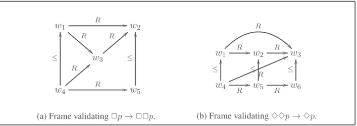
property of transitivity of a frame. It is also canonical, seeing that K + ✷p → ✷✷p has a transitive canonical frame. The formula ✸✸p → ✸p possesses these properties as well — correspondence and canonicity. Within the context of the birelational semantics, neither ✷p → ✷✷p, nor ✸✸p → ✸p corresponds to transitivity. In fact, on one hand, the strongly normal frame shown in Figure 1a is non-transitive and, moreover, it validates ✷p → ✷✷p.
w1 R !! R //w2 w3 R == w4 R == R // ≤ OO w5 ≤ OO
(a) Frame validating ✷p → ✷✷p.
w1 R // R w2 R //w3 w4 R 66 R // ≤ OO w5 R // ≤ OO w6 ≤ OO (b) Frame validating ✸✸p → ✸p.
Figure 1: Non-transitive and strongly normal frames
On the other hand, the strongly normal frame shown in Figure 1b is non-transitive and it validates ✸✸p → ✸p. The thing is that we do not know if there exists a formula ϕ such that for all strongly normal birelational frames (W, ≤, R), R is transitive if (W, ≤, R) validates
ϕ. Nevertheless,
Lemma 20. The canonical frame ofK4HT = KHT + (✷p → ✷✷p) ∧ (✸✸p → ✸p) is transitive.
Proof. Let x, y, z be arbitrary prime theories such that xRcy and yRcz. Hence, ✷x ⊆ y,
✸y ⊆ x, ✷y ⊆ z and ✸z ⊆ y. Let ϕ be a formula such that ✷ϕ ∈ x. Since ✷ϕ → ✷✷ϕ ∈
x, ✷x ⊆ y, and ✷y ⊆ z, we have that ✷✷ϕ ∈ x, ✷ϕ ∈ y and ϕ ∈ z. Consequently,
✷x ⊆ z. Similarly, on can easily show that ✸z ⊆ x, this time using a formula of the form ✸✸ϕ → ✸ϕ. As a result, xRcz. Since x, y, z were arbitrary, we conclude that Rc is
transitive.
To the best of our knowledge, the equivalent to the Sahlqvist correspondence theorem for modal extensions of here and there (and even for Simpson’s intuitionistic modal logic K [39]) was not considered in the literature. Extending Sahlqvist’s result to our setting would help us to prove the completeness for extensions of KHT .
6
About bisimulations
In modal logic, bisimulations are binary relations between models that relate possible worlds carrying the same modal information. However the classical definition of bisimulation must be relaxed in the case of KHT . In this section we provide a definition of bisimulation in the case of KHT , which is sufficient to prove the corresponding bisimulation lemma that states that if two models are bisimilar then they satisfy the same formulas.
6.1 Bisimulations for KHT
Let M1 = éW1, R1, H1, T1ê and M2 = éW2, R2, H2, T2ê be KHT -models. Let D1 =
W1×{h, t} and D2 = W2×{h, t}. A binary relation Z between D1and D2is a bisimulation
if the following conditions are satisfied:
1) if (x1, α1)Z(x2, α2) then M1,(x1, α1) |= p iff M2,(x2, α2) |= p for all propositional
variables p;
2) if (x1, α1)Z(x2, α2) then (x1, t)Z(x2, t);
3) if (x1, α1)Z(x2, α2) and x1R1y1 then there exists y2 ∈ W2 such that x2R2y2 and
either (y1, α1)Z(y2, α2) or (y1, t)Z(y2, α2);
4) if (x1, α1)Z(x2, α2) and x2R2y2 then there exists y1 ∈ W1 such that x1R1y1 and
either (y1, α1)Z(y2, α2) or (y1, α1)Z(y2, t);
5) if (x1, α1)Z(x2, α2) and x2R2y2 then there exists y1 ∈ W1 such that x1R1y1 and
either (y1, α1)Z(y2, α2) or (y1, t)Z(y2, α2);
6) if (x1, α1)Z(x2, α2) and x1R1y1 then there exists y2 ∈ W2 such that x2R2y2 and
either (y1, α1)Z(y2, α2) or (y1, α1)Z(y2, t).
Lemma 21 (Bisimulation Lemma). Let M1 = éW1, R1, H1, T1ê and M2 = éW2, R2,
H2, T2ê be KHT -models. Let D1 = W1 × {h, t} and D2 = W2 × {h, t}. Let Z be a
bisimulation betweenD1 andD2 and letϕ be a formula. For all(x1, α1) ∈ D1 and for all
(x2, α2) ∈ D2, if(x1, α1)Z(x2, α2) then M1,(x1, α1) |= ϕ iff M2,(x2, α2) |= ϕ.
Proof. By induction on ϕ. We only consider the cases ϕ → ψ, ✸ϕ and ✷ϕ.
• ϕ → ψ: Suppose (x1, α1)Z(x2, α2), M1,(x1, α1) |= ϕ → ψ. From the former
assumption and Condition 2) we conclude (x1, t)Z(x2, t). From the latter assumption
it follows that for all α′
1 ∈ {α1, t}. M, (x1, α′1) Ó|= ϕ or M, (x1, α′1) |= ψ. If α′1 = α1
then, by (x1, α1)Z(x2, α2) and induction hypothesis we get M, (x2, α2) Ó|= ϕ or
M, (x2, α2) |= ψ. If α′1 = t then, by (x1, t)Z(x2, t) and the induction hypothesis, we
get M, (x2, t) Ó|= ϕ or M, (x2, t) |= ψ. From this it follows that M, (x2, α2) |= ϕ →
ψ. The converse direction is proved in a similar way.
• ✸ϕ: Suppose (x1, α1)Z(x2, α2) and M1,(x1, α1) |= ✸ϕ. Let y1 ∈ W1 be such that
x1R1y1 and M1,(y1, α1) |= ϕ. By Lemma 1, M1,(y1, t) |= ϕ holds as well. By
Condition 3) and the induction hypothesis it follows that M2,(y2, α2) |= ϕ for some
y2 ∈ W2 satisfying x2R2y2. Therefore M2,(x2, α2) |= ✸ϕ. The converse direction
• ✷ϕ: Suppose (x1, α1)Z(x2, α2) and M2,(x2, α2) Ó|= ✷ϕ. Let y2 ∈ W2 be such
that x2R2y2 and M2,(y2, α2) Ó|= ϕ. By Lemma 1, Condition 5) and the induction
hypothesis it follows that M1,(y1, α1) Ó|= ϕ for some y1 ∈ W1 satisfying x1R1y1.
Therefore M1,(x1, α1) Ó|= ✷ϕ. The converse direction is proved in a similar way but
using Condition 6).
Obviously, the union of two bisimulations is also a bisimulation. Hence, there exists a maximal bisimulation Zmax between D1 and D2.
6.2 Interdefinability of Modal Operators
As an application of bisimulation, in this section we prove that ✷ and ✸ are not interdefin-able. To do so, we introduce the concepts of ✷-free and ✸-free bisimulations. Let M1 =
éW1, R1, H1, T1ê and M2 = éW2, R2, H2, T2ê be KHT -models. Let D1 = W1 × {h, t}
and D2 = W2× {h, t}. A binary relation Z between D1 and D2 is a ✷-free-bisimulation if
it satisfies conditions 1)-4) of bisimulations. In the same way, a binary relation Z between
D1 and D2 is a ✸-free-bisimulation if it satisfies conditions 1)-2) and 5)-6) of bisimulations.
Proposition 5. Let M1 andM2 beKHT -models, D1 = W1× {h, t}, D2 = W2 × {h, t}
andZ be a binary relation between D1 andD2.
• If Z is a ✸-free-bisimulation then M1 andM2 satisfy the same ✸-free formulas;
• If Z is a ✷-free-bisimulation then M1 andM2 satisfy the same ✷-free formulas.
Proof. Similar to the proof of the Bisimulation Lemma.
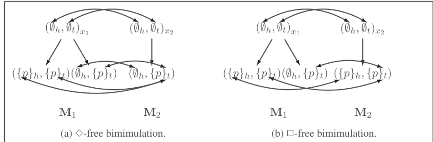
To show that ✸ is not definable in terms of ✷, let us consider the models shown in Figure 2a. It can be checked that M1,(x1, h) |= ✸p but M2,(x2, h) Ó|= ✸p. However, as
shown in such figure, there exists a ✸-free-bisimulation between them. As a result, Proposition 6. There is no ✸-free formula ϕ such that |= ✸p ↔ ϕ.
Proof. We proceed by contradiction. Assume that such ϕ exists. Let us consider the models M1and M2 together with the points x1 and x2from Figure 2a. Note that M1,(x1, h) |= ✸p.
Therefore M1,(x1, h) |= ϕ. Thanks to Proposition 5 and the ✸-free bisimulation described
in Figure 2a, M2,(x2, h) |= ϕ. As a consequence, M2,(x2, h) |= ✸p: a contradiction.
To show that ✷ is not definable in terms of ✸, we consider the models presented in Figure 2b, in which M2,(x2, h) |= ✷p and M1,(x1, h) Ó|= ✷p. As shown in such figure, there exists a
(∅h,∅t)x1
({p}h,{p}t)(∅h,{p}t)
(∅h,∅t)x2
(∅h,{p}t)
M1 M2
(a) ✸-free bimimulation.
(∅h,∅t)x1 ({p}h,{p}t)(∅h,{p}t) (∅h,∅t)x2 ({p}h,{p}t) M1 M2 (b) ✷-free bimimulation.
Figure 2: ✸-free and ✷-free bimimulations. Proposition 7. There is no ✷-free formula ϕ such that |= ✷p ↔ ϕ.
Proof. We proceed by contradiction. Assume that such ϕ exists. Let us consider the models M1and M2 together with the points x1 and x2from Figure 2b. Note that M1, (x1, h) Ó|= ✷p.
Consequently, M1, (x1, h) Ó|= ϕ. Thanks to Proposition 5 and the ✷-free bisimulation
described in Figure 2b, M2, (x2, h) Ó|= ϕ. As a consequence, M2, (x2, h) Ó|= ✷p: a
contradiction.
6.3 Hennessy-Milner property
In order to show that our definition of bisimulation is appropriate, in this section we show that KHT possesses the Hennessy-Milner property. Our proof follows the line of reasoning suggested in [30]. Let M1 = éW1, R1, H1, T1ê and M2 = éW2, R2, H2, T2ê be finite
KHT models. Let D1 = W1 × {h, t} and D2 = W2 × {h, t}. We define the binary
relation ! between D1 and D2 as follows: (x1, α1) ! (x2, α2) if for all formulas ϕ,
M1, (x1, α1) |= ϕ iff M2, (x2, α2) |= ϕ.
Lemma 22 (Hennesy-Milner property). The binary relation ! is a bisimulation between M1 and M2.
Proof. Suppose that the binary relation ! is not a bisimulation. Hence, by Lemma 21, one of the conditions 1)-6) does not hold for some (x1, α1) ∈ D1 and some (x2, α2) ∈ D2 such
that (x1, α1) ! (x2, α2).
Assume that Condition 1) is not satisfied. Hence there exists an atom p such that, without loss of generality, M1, (x1, α1) |= p and M2, (x2, α2) Ó|= p. Therefore not (x1, α1) !
(x2, α2): a contradiction.
Assume that Condition 2) is not satisfied. Thus (x1, α1) ! (x2, α2) and not (x1, t) !
(x1, t) |= ϕ and M2,(x2, t) Ó|= ϕ. Thus M1,(x1, α1) Ó|= ¬ϕ and M2,(x2, α2) |= ¬ϕ: a
contradiction.
Assume that Condition 3) is not satisfied: Then (x1, α1) ! (x2, α2) and there exists
y1 ∈ W1 such that x1R1y1 and for all y2 ∈ W2, if x2R2y2 then not (y1, α1) ! (y2, α2)
and not (y1, t) ! (y2, α2). Let R2(x2)
def
= {(y2, α2) ∈ D2 | x2R2y2}. Since for all
y2 ∈ W2, if x2R2y2 then not (y1, α1) ! (y2, α2) and not (y1, t) ! (y2, α2), there exist
I, J ⊆ R2(x2) and for all (y2, α2) ∈ R2(x2) there exist formulas ϕ(y2, α2) and ψ(y2, α2)
such that
1) M1,(y1, α1) |= ϕ(y2, α2) and M2,(y2, α2) Ó|= ϕ(y2, α2) if (y2, α2) ∈ I;
2) M1,(y1, α1) Ó|= ϕ(y2, α2) and M2,(y2, α2) |= ϕ(y2, α2) if (y2, α2) ∈ I;
3) M1,(y1, t) |= ψ(y2, α2) and M2,(y2, α2) Ó|= ψ(y2, α2) if (y2, α2) ∈ J;
4) M1,(y1, t) Ó|= ψ(y2, α2) and M2,(y2, α2) |= ψ(y2, α2) if (y2, α2) ∈ J.
Let us define χ(y2, α2) as the following formula:
χ(y2, α2) = ϕ(y2, α2) if (y2, α2) ∈ I; ϕ(y2, α2) → ψ(y2, α2) if (y2, α2) ∈ I ∩ J; ¬ψ(y2, α2) if (y2, α2) ∈ I ∩ J.
It follows that M1,(y1, α1) |= χ(y2, α2) and M2,(y2, α2) Ó|= χ(y2, α2), for all (y2, α2) ∈
R2(x2). Therefore M1,(x1, α1) |= ✸ Þ (y2,α2)∈R2(x2) χ(y2, α2) while M2,(x2, α2) Ó|= ✸ Þ (y2,α2)∈R2(x2) χ(y2, α2) : a contradiction.
The proof for Condition 4) is similar to the proof of Condition 3)
Assume that Condition 5) is not satisfied: Then (x1, α1) ! (x2, α2) and there exists
y2 ∈ W2 such that x2R1y2 and for all y1 ∈ W1, if x1R1y1 then not (y1, α1) ! (y2, α2)
and not (y1, t) ! (y2, α2). Let R1(x1)
def
= {(y1, α1) ∈ D1 | x1R2y1}. Since for all
y1 ∈ W1, if x1R1y1 then not (y1, α1) ! (y2, α2) and not (y1, t) ! (y2, α2), there exist
I, J ⊆ R1(x1) and for all (y1, α1) ∈ R1(x1) there exist formulas ϕ(y1, α1) and ψ(y1, α1)
such that
2) M1,(y1, α1) Ó|= ϕ(y1, α1) and M2,(y2, α2) |= ϕ(y1, α1) if (y1, α1) ∈ I;
3) M1,(y1, t) |= ψ(y1, α1) and M2,(y2, α2) Ó|= ψ(y1, α1) if (y1, α1) ∈ J;
4) M1,(y1, t) Ó|= ψ(y1, α1) and M2,(y2, α2) |= ψ(y1, α1) if (y1, α1) ∈ J.
Let us define χ(y1, α1) as the following formula:
χ(y1, α1) def = ϕ(y1, α1) if (y1, α1) ∈ I; ϕ(y1, α1) → ψ(y1, α1) if (y1, α1) ∈ I ∩ J; ¬ψ(y1, α1) if (y1, α1) ∈ I ∩ J.
It follows that M1,(y1, α1) |= χ(y1, α1) and M2,(y2, α2) Ó|= χ(y1, α1), for all (y1, α1) ∈
R1(x1). Therefore M1,(x1, α1) |= ✸ Þ (y1,α1)∈R1(x1) χ(y1, α1) while M2,(x2, α2) Ó|= ✸ Þ (y1,α1)∈R1(x1) χ(y1, α1) : a contradiction.
The proof for Condition 6) is similar to the proof for Condition 5).
Remark how the formulas defining χ above are related to the Hosoi Axiom p ∨ (p → q) ∨ ¬q.
7
Strong equivalence property
Pearce’s Equilibrium logic [33] is the best-known logical characterization of the stable models semantics [23] and of Answer Sets [7]. It is defined in terms of the monotonic logic of Here and There [34] (HT) plus a minimisation criterion among the given models. This simple definition led to several modal extensions of Answer Set Programming [11, 16]. All these extensions have their roots in the corresponding modal extensions of HT-logic defined as the combination of propositional HT and any modal logic [22] that play an important role in the proof of several interesting properties of the resulting formalisms such as strong equivalence [10, 16, 29] and the complexity [5, 9]. Although the modal extensions of the HT-logic have been studied only in concrete cases such as the Linear Time Temporal
KHT -logic [2], the lack of a general theory that allows defining such modal HT extension
as well as extending the concept of equilibrium model to modal case caught our attention. In this section, we define the concept of pointed equilibrium model and prove the associated theorem of strong equivalence.
Let M = éW, R , H, T ê be a KHT model. A KHT pointed model is a pair (M, x) where x ∈ W . (M, x) is said to be total if H = T . Moreover, by the expression H <x
k T
we mean that there exists y ∈ W and 0 ≤ k such that xRky and H(y) Ó= T (y). A total
KHT pointed model(M, x) is a pointed equilibrium model of a formula ϕ if
1) M, (x, h) |= ϕ;
2) For all KHT models M′ = éW, R, H′, Tê3 and for all 0 ≤ k ≤ deg(ϕ) if H′ <x k T
then M′,(x, h) Ó|= ϕ.
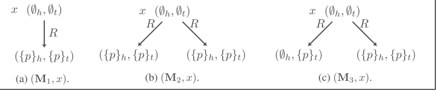
As an example, let us consider the three models displayed in Figure 3. (M1, x), (M2, x)
and (M3, x) correspond to three different KHT pointed models of the formula ✸p. For each
Kripke world, the “here” component is represented with the subscript h and the “there” part is done by the subscript t. While (M1, x) is a pointed equilibrium model (i.e. it is total and
minimal with respect to <x
0 and <x1, M2 is not. Although (M2, x) is a total KHT pointed
model satisfying ✸p, it does not satisfy Condition 2) being (M3, x) a counterexample.
(∅h,∅t) x ({p}h,{p}t) R (a) (M1, x). (∅h,∅t) x ({p}h,{p}t) ({p}h,{p}t) R R (b) (M2, x). (∅h,∅t) x ({p}h,{p}t) (∅h,{p}t) R R (c) (M3, x).
Figure 3: Three KHT pointed models satisfying ✸p.
Lemma 23. Let M = éW, R, H, T ê be a KHT model and letM = éW, R, T, T ê denoteã its corresponding total model. LetΓ0
def
= {✷k(p ∨ ¬p) | 0 ≤ k and p ∈ V AR} be a theory.
For allKHT pointed models(M, x), M, (x, h) |= Γ0 iff for allk ≥ 0, H Ó<xk T .
Proof. From left to right, assume by contradiction that H <xk T for some k ≥ 0. Therefore, there exists y ∈ W such that xRky and H(y) Ó= T (y). Let p ∈ V AR be such that
p ∈ (T (y) \ H(y)). It can be checked that M, (y, h) Ó|= (p ∨ ¬p). Since xRky we get
M, (x, h) Ó|= ✷k(p ∨ ¬p). As a consequence, M, (x, h) Ó|= Γ0: a contradiction. Conversely,
assume that M, (x, h) Ó|= Γ0, so M, x Ó|= ✷k(p ∨ ¬p) for some 0 ≤ k. This means that
there exists y ∈ W such that xRky and M, (y, h) Ó|= p ∨ ¬p, so H(y) Ó= T (y). Therefore,
H <xk T : a contradiction.
3
Two theories Γ1 and Γ2 are KHT -equivalent (in symbols Γ1 ≡KHT Γ2) if they have the
same KHT pointed models. A total KHT pointed model (M, x) is a pointed equilibrium modelof a theory Γ if
1) M, (x, h) |= Γ;
2) For all KHT models M′ = éW, R
,H′, Tê and for all 0 ≤ k ≤ deg(Γ), if H′ <xk T
then M′,(x, h) Ó|= Γ.
When dealing with non-monotonicity the relation of equivalence between theories depends on the context where they are considered. We say that two theories Γ1 and Γ2 are strongly
equivalent[29] (in symbols Γ1 ≡s Γ2) if for all theories Γ, Γ1∪ Γ and Γ2∪ Γ have the same
pointed equilibrium models.
Proposition 8. For all theories Γ1 and Γ2 such that deg(Γ1) = deg(Γ2), Γ1 ≡s Γ2 iff
Γ1 ≡KHT Γ2.
Proof. From right to left, suppose Γ1 ≡KHT Γ2 and let Γ be an arbitrary theory.
Conse-quently, (Γ1∪ Γ) ≡KHT (Γ2 ∪ Γ) so Γ1∪ Γ and Γ2∪ Γ have the same pointed equilibrium
models.
From left to right, suppose that Γ1 and Γ2 are strongly equivalent but they are not KHT
-equivalent. Let Γ0
def
= {✷k(p ∨ ¬p) | 0 ≤ k and p ∈ V AR}.
• First case: Γ1 and Γ2 are not K-equivalent. Without loss of generality, there exists a
total KHT pointed model (M, x), with M = éW, R, T, T ê, such that M, (x, h) |= Γ1
but M, (x, h) Ó|= Γ2. It can be checked that (M, x) is a pointed equilibrium model of
Γ1∪ Γ0 but not of Γ2 ∪ Γ0.
• Second case: Γ1 and Γ2 are K-equivalent. Therefore, without loss of generality,
there exists a KHT model M = éW, R, H, T ê (whose corresponding total model is denoted byM = éW, R, T, T ê) and x ∈ W such thatã
(1) M, (x, t) |= Γ1 iff M, (x, t) |= Γ2 because both Γ1 and Γ2 are K-equivalent;
(2) M, (x, h) |= Γ1 and M, (x, h) Ó|= Γ2 because Γ1 and Γ2 are not KHT
-equivalent;
Since M, (x, h) Ó|= Γ2, there exists ϕ ∈ Γ2 such that M, (x, h) Ó|= ϕ. Since
M, (x, t) |= Γ2 then M, (x, t) |= ϕ. Since M, (x, h) Ó|= ϕ, therefore, there exits
0 ≤ k ≤ deg(ϕ) such that H <xk T . Let Γ def= {ϕ → ψ | ψ ∈ Γ0}. Note that
M, (x, h) |= Γ1 ∪ Γ since M, (x, h) |= Γ1, M, (x, h) Ó|= ϕ and M, (x, t) |= Γ0.
ã
M, (x, h) |= Γ1∪Γ and H <xk T , where k≤ deg(Γ1∪Γ). As a result, (M, x) is not aã
pointed equilibrium model of Γ1∪ Γ. Since Γ1 and Γ2 are strongly equivalent, (M, x)ã
is not a pointed equilibrium model of Γ2 ∪ Γ. Since Γ1 and Γ2 are K-equivalent,
Γ1 ∪ Γ and Γ2 ∪ Γ are K-equivalent. Hence, M, (x, h) |= Γã 2 ∪ Γ. Since (M, x)ã
is not a pointed equilibrium model of Γ2 ∪ Γ, there exists M′ = éW, R,H′, Tê and
0 ≤ k′ ≤ deg(Γ
2 ∪ Γ) such that H′ <xk′ T and M′,(x, h) |= Γ2 ∪ Γ. However, from M′,(x, h) |= Γ2 ∪ Γ and the fact that ϕ ∈ Γ2, it follows that M′,(x, h) |= Γ0. Thus,
by Lemma 23, H′
✚<✚xk′T : a contradiction.
The theorem plays an important role in the area of Answer Set Programming [7] since it allows, under ASP semantics, to exchange two logic programs (or theories) regardless the context in which they are considered. This theorem also justifies the use of KHT as a monotonic basis supporting non-monotonicity.
8
Conclusion
In this paper, we have introduced and studied a combination of the logic of Here and There and modal logic for which we have obtained several results such as non-interdefinability of modal operators, complexity of the satisfiability problem, finite model property or axiomati-sation. However, there is still a lot of open lines of research we want to study:
1) Other combinations of the logic of Here and There and modal logic: S4 − HT ,
P DL− HT , CT L − HT , etc;
2) Decision procedures, based on tableau methods, for the aforementioned logics; 3) Van Benthem characterisation theorem [3] for combinations of the logic of Here and
There with modal logic;
4) An expressive completeness result similar to Kamp’s result [21] in the setting of
LT L-HT .
5) The logic FS was defined by G. Fisher Servi so that ϕ ∈ F S iff the standard translation
STx(ϕ) is a tautology of first order intuitionistic logic. Checking if the same relation
holds in the Here and There case will be considered in the near future.
Acknowledgements
We make a point of thanking our referees for their valuable remarks and their helpful feedback.
References
[1] F. Aguado, P. Cabalar, G. Pérez, C. Vidal, Strongly equivalent temporal logic programs, in: JELIA’08, 2008.
[2] P. Balbiani, M. Diéguez, Temporal Here and There, in: JELIA’16, 2016.
[3] J. van Benthem, Correspondence theory, in: Handbook of Philosophical Logic: Volume II: Extensions of Classical Logic, Reidel, 1984, pp. 167–247.
[4] P. Blackburn, M. de Rijke, Y. Venema, Modal Logic, Cambridge University Press, 2001. [5] L. Bozzelli, D. Pearce, On the complexity of temporal equilibrium logic, in: LICS’15, 2015. [6] M. Boži´c, K. Došen, Models for normal intuitionistic modal logics, Studia Logica 43 (3) (1984)
217–245.
[7] G. Brewka, T. Eiter, M. Truszczy´nski, Answer set programming at a glance, Commun. ACM 54 (12) (2011) 92–103.
[8] R. A. Bull, A modal extension of intuitionist logic, Notre Dame Journal of Formal Logic 6 (2) (1965) 142–146.
[9] P. Cabalar, S. Demri, Automata-based computation of temporal equilibrium models, in: LOP-STR’11, 2011.
[10] P. Cabalar, M. Diéguez, Strong equivalence of non-monotonic temporal theories, in: KR’14, 2014.
[11] P. Cabalar, G. Pérez, Temporal Equilibrium Logic: a first approach, in: EUROCAST’07, 2007. [12] A. Chagrov, M. Zakharyaschev, Modal Logic, Oxford University Press, 1997.
[13] E. M. Clarke, E. A. Emerson, A. P. Sistla, Automatic verification of finite-state concurrent systems using temporal logic specifications, ACM Trans. Program. Lang. Syst. (1986) 244–263. [14] L. Esakia, On varieties of Grzegorczyk algebras, Studies in Non-Classical Logics and Set
Theory (1979) 257–287.
[15] M. Fairtlough, M. Mendler, An intuitionistic modal logic with applications to the formal verification of hardware, in: CSL’94, Springer, 1995.
[16] L. Fariñas del Cerro, A. Herzig, E. Su, Epistemic Equilibrium Logic, in: IJCAI’15, 2015. [17] G. Fischer Servi, On modal logic with an intuitionistic base, Studia Logica 36 (3) (1977)
141–149.
[18] G. Fischer Servi, Semantics for a Class of Intuitionistic Modal Calculi, chap. 5, Springer, 1981, p. 59–72.
[19] G. Fischer Servi, Axiomatizations for some intuitionistic modal logics, in: Rendiconti del Seminario Matematico Università e Politecnico di Torino, No. 42 in 3, 179–194, 1984.
[20] F. B. Fitch, Natural deduction rules for obligation, American Philosophical Quarterly 3 (1) (1966) 27–38.
[21] D. Gabbay, I. Hodkinson, M. Reynolds, Temporal Logic: Mathematical Foundations and Computational Aspects, No. vol. 1 in Oxford logic guides, Clarendon Press, 1994.
[22] D. Gabbay, A. Kurucz, F. Wolter, M. Zakharyaschev, Many-Dimensional Modal Logics: Theory and Applications, North Holland, 2003.