Skyrmions dans la simple couche et la bicouche de graphène

Wenchen Luo

A thesis submitted to the physics department in accordance with the requirements of the degree of

Master of Science in the Faculty of Science.

FACULTE DES SCIENCES UNIVERSITE DE SHERBROOKE

1*1

Your Tile Votre reference ISBN: 978-0-494-53180-8 Our file Notre reference ISBN: 978-0-494-53180-8

NOTICE: AVIS:

The author has granted a

non-exclusive license allowing Library and Archives Canada to reproduce, publish, archive, preserve, conserve, communicate to the public by

telecommunication or on the Internet, loan, distribute and sell theses

worldwide, for commercial or non-commercial purposes, in microform, paper, electronic and/or any other formats.

L'auteur a accorde une licence non exclusive permettant a la Bibliotheque et Archives Canada de reproduire, publier, archiver, sauvegarder, conserver, transmettre au public par telecommunication ou par I'lnternet, prefer, distribuer et vendre des theses partout dans le monde, a des fins commerciales ou autres, sur support microforme, papier, electronique et/ou autres formats.

The author retains copyright ownership and moral rights in this thesis. Neither the thesis nor substantial extracts from it may be printed or otherwise reproduced without the author's permission.

L'auteur conserve la propriete du droit d'auteur et des droits moraux qui protege cette these. Ni la these ni des extraits substantiels de celle-ci ne doivent etre imprimes ou autrement

reproduits sans son autorisation.

In compliance with the Canadian Privacy Act some supporting forms may have been removed from this thesis.

Conformement a la loi canadienne sur la protection de la vie privee, quelques

formulaires secondaires ont ete enleves de cette these.

While these forms may be included in the document page count, their removal does not represent any loss of content from the thesis.

Bien que ces formulaires aient inclus dans la pagination, il n'y aura aucun contenu manquant.

1*1

Wenchen Luo

Memoire presente au Departement de physique en vue de l'obtention du grade de Maitre es sciences (M.Sc.)

FACULTE DES SCIENCES UNIVERSITE DE SHERBROOKE

Le29juillet2009

lejury a accepte le memoire de M. Wenchen Luo dans sa version finale.

Membres dujury M. Rene Cote Directeur Departement de physique M. Alexandre Blais Membre Departement de physique M. Mario Poirier President-rapporteur Departement de physique

R e s u m e

Le graphene, une monocouche de graphite, n'a ete isole qu'en 2004 par Novoselov et al. [2]. Depuis ce temps, le graphene a ete le sujet de nombreuses recherches tant theoriques qu'experimentales. Dans cette these, nous etudions l'etat fondamental du gaz d'electrons bidimensionnel (GE2D) en champ magnetique intense dans un systeme avec une seule couche de graphene ainsi que dans un systeme forme de deux couches superposees de graphene (une bicouche). Nous nous concentrons tout d'abord sur les phases liquides qui se produisent aux remplissages entiers v — 1, 2, 3, 4 en incluant les degres de liberte de spin et de pseudo-spin puis sur des phases cristallines appelees cristaux de merons qui se produisent autour du remplissage u = 1 dans le graphene. Nous calculous ensuite l'energie necessaire pour exciter un seul skyrmion ou antiskyrmion avec une texture de pseudospin au remplissage v = — 3 dans la bicouche de graphene. Notre calcul montre que ces excitations topologiques ont une energie plus elevee que celle correspondant a l'excitation d'un electron ou d'un trou sans texture au remplissage v = — 1. Nous en concluons que ces excitations topologiques ne jouent pas un role dominant dans la conductivite de la bicouche a v = — 3.

the meron crystal phases with spin and valley pseudospin textures around filling factor

v = 1. We then look for single-particle excitations in a bilayer graphene system at the

filling factor v = — 3. We find that charged pseudo-spin textures do not exist in such a system. The lowest charged excitations are the quasi-hole and quasi-electron states. We conclude that topological excitations do not play a significant role in the conductivity of the bilayer at v = — 3.

Acknowledgement

I would like to thank my supervisor Prof. Rene Cote for his enthusiastic help on my research work and study. I also appreciate his revision of this thesis in content and grammar.

I also would like to thank my parents, uncle and aunt. Without their help, I could not reach Canada to proceed my study. My uncle and aunt who live in Sherbrooke also give me much help in my daily life. I appreciate them very much.

At last, I would like to thank my friends, Jules Lambert, Jean-Frangois Jobidon, Marc-Antoine Lemonde, Branko Petrov for their helpful discussion.

List of Figures ix Introduction 1 1 The concept of skyrmion in quantum Hall system 4

•1.1 Classical and quantum Hall effects 4

1.1.1 Classical Hall effect 4 1.1.2 Quantum Hall Effect 7 1.2 Topological soliton: skyrmion and antiskyrmion 8

1.2.1 Soliton and solitary wave 8 1.2.2 Topological soliton solution of the nonlinear sigma model 12

2 Single particle excitations in monolayer quantum Hall system 19

2.1 Hamiltonian of the system in the Hartree-Fock approximation 21

2.2 Quasi-hole and quasi-particle states 25

2.3 Spin textures 27

3 Quantum Hall crystal phases in monolayer graphene 34

3.1 Introduction to graphene 35 3.1.1 Crystal structure 35

3.2 Band structure 37

Contents viii

3.2.1 QHE in graphene 41 3.3 Second quantized hamiltonian of the 2DEG in the Hartree-Fock

approxi-mation 46 3.4 Equation of motion for the single-particle Green's function 50

3.5 Liquid phases at v = 1,2,3,4 55 3.6 Electronic crystals in graphene with spins 58

4 Single-particle excitations in bilayer graphene 62

4.1 Geometrical structure and other properties 62

4.2 Effective two-band model 64 4.2.1 Effective hamiltonian for the case 72 = 73 = 0 and finite bias . . . 65

4.2.2 Eigenvalues of the effective two-band model in the presence of a

magnetic field 65 4.3 Single-particle excitations at v = — 3 and A# > A^ 68

4.3.1 Single-particle excitation states 70 4.3.2 The quasi-hole and quasi-electron states 73

4.3.3 The possibility of orbital pseudo-spin texture states 74

Conclusion 78 A Landau level 80 B Fermion canonical transformation 83

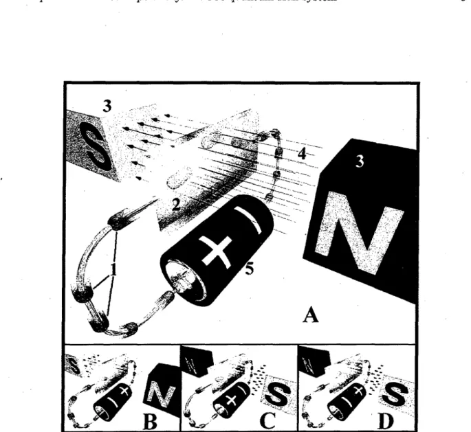
Hall effect takes on a negative charge at the top edge and a positive charge at the lower edge of the conducting medium "2" in "A". In "B" and "C", the polarization is reversed because of the reversal of the electric current or the magnetic field. For case "D", both current and magnetic field are

reversed, which means the polarization is the same as "A" 5

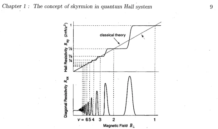
1.2 A Hall effect scheme. 6 1.3 Hall resistivity contrast between classical Hall effect and quantum Hall

effect. This picture is cited from [6]. 9

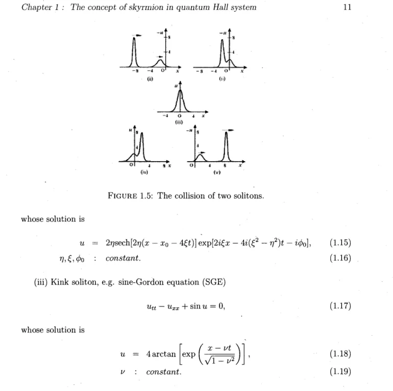
1.4 Soliton in life, kink ice [19] 10 1.5 The collision of two solitons . 11

1.6 A kink and an anti-kink 12 1.7 (f)°° defines the mapping from S1 to another S1. A point in the real space

(normal U(l) group) eld is mapped to the point in ve1^6"1 in the field space

uniquely by (jf°. This is nontrivial. 13 1.8 A mapping from U(l) (Sl circle) to a S2 sphere. The mapped circle in

S2 is still a closed curved line that can be continuously shrunk to a point,

which means the mapping is trivial. 14 1.9 Firstly, compact the xOy plane (R2) to a S2 (in a 3D frame) sphere only

except the north pole where the boundary condition takes value. Then mapping from the S2 to another S2 (a sphere based on 3 components of

the field) is nontrivial, 7T2 (S2) ^ 0 15

List of Figures x

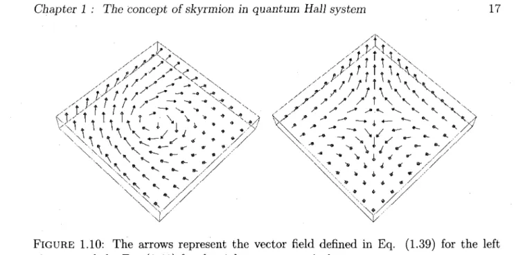
1.10 The arrows represent the vector field defined in Eq. (1.39) for the left

picture, and the Eq. (1.41) for the right one, respectively 17 2.1 The spin generated ground state (Landau level n — 0) at filling factor

v = 1 is split by the external magnetic field B. The gap between two

levels is the Zeeman bias AB = gfisB, where g is Lande factor and (XB

is the Bohr magneton. Each blue ball represents one electron at angular

momentum m = 0,1, 2 , . . . from left to right respectively 20 2.2 Quasi-hole state in the left picture and quasi-electron state in the right one. 21

2.3 The upper picture sketches the antiskyrmion state (Eq. 2.12) where ao is removed. And the lower one represents the skyrmion state (Eq. 2.13), the blue dot is the added electron %. The BCS-like pairs are formed in spin

texture states 28 2.4 Density and spin texture of an antiskyrmion. The pictures of this

numer-ical experiment is done under Zeeman bias gfiBB/2 = 0.01, in which all

2

lengths are in units of £ and energies are in units of ^ . In all of these

numerical computation, only the parameter of Zeeman bias is tunable. . . 31 2.5 Spin texture of skyrmion. All conditions and units are the same as those

shown in the case of antiskyrmion in Fig. 2.4 • • • • 32 2.6 Excitation energy comparison between quasi-electron states and spin

tex-tures at different Zeeman bias 33 2.7 The energy comparison between two kinds of single-particle excitations

at small Zeeman couplings. The red line represents the energy Ae/, to excite a quasi-hole and quasi-particle pair (given in Eq. (2.28)), while the green curve is the energy (computed numerically) to excite a

skyrmion-antiskyrmion pair 33 3.1 Graphene crystal lattice. Each red atom is linked to its three nearest

neighbors by vectors &!, 62,63. The C atoms can be separated into two kinds of atoms denoted by red (^4) and blue (B) dots, i.e. we can divide

the whole lattice into two sublattice whose lattice vectors are ai and a i . 36 3.2 Reciprocal lattice based on { b i , b2} and the first Brillouin zone

repre-sented by the red regular hexagon 37 3.3 Energy band or dispersion relation and the Dirac's cone 40

Fig. 3.5. The parameters of the system are: n — 0 Landau level, Zeeman coupling 7 = 10~4 in units of ^ , and the filling factor v = 1.3. Because of the Zeeman gap, the spin merons in each valley is not a perfect meron,

Sz G [—0.15,0.3]. But the valley merons in both spin up and down are

still perfect ones 60 3.7 Total spin polarization curves at different filling factors. Sp = T 2 l. The

2

x-axis represents the Zeeman coupling in units of ~v 61

4.1 The geometry structure of bilayer graphene in the Bernal stacking. There are two sublattices in each layer: A\ and B\ for the top layer (the red

lattice); A<i and B2 for the bottom layer (the green one) 63

4.2 Dispersion relations around the K valley. . . 65 4.3 In a magnetic field, the conduction and valence bands are split to quantized

Landau levels. The ground state is the Fermi level (red line) lies in the

middle of n = 0 Landau level 68 4.4 The four levels of the ground state without Coulomb interaction. If there

is no bias, the ground state is 4-fold degenerate. The valley pseudo-spin

is polarized even for a very small bias 69 4.5 The ferromagnetism ground state with no bias (A# = 0) in the symmetric

gauge, hw is the energy gap between the lowest and the second Landau level, which is given in Appendix A. n' represents the index of sub Landau

level, and m represents the angular momentum number 69 4.6 Sketch drawing of electron pairing. The upper picture represents the pairs

in the anti-skyrmion state of Eq. (4.23a), and the lower one represents the pairs in the skyrmion state of Eq. (4.23b). The topological charge of this

Figures

The top and bottom pictures show the quasi-hole and quasi-electron states, respectively

With a negative bias, sub Landau levels in the K valley go down while levels in the K' valley go up. At the liquid phase of filling factor v = — 1, the K valley is full filled with electrons. Because — /3AB is still smaller than the natural gap between 0 and 1 sub Landau levels, the sub Landau level n' = 0 in the K' valley is full filled while the other level in K' valley is empty. . .

layer of graphite may be produced during normal writing, it was only isolated in 2004 [1] and studied extensively since then [3]. We, call the single layer of graphite "graphene". A graphene sheet is a good system to study a two dimensional electron gas.

The two-dimension electron gas (2DEG) has already been studied a lot in semicon-ductor microstructures. One of its most important properties is the quantum Hall effect (integer and fractional) which is the quantization of the conductivity axy in the presence

of magnetic field.

For a conventional 2DEG in a magnetic field, the ground state at filling factor v = 1 is a ferromagnet because of the Coulomb interactions. The lowest-energy single-particle excitations are spin texture states instead of quasi-electron or quasi-hole states at small Zeeman coupling [4,5]. The spin texture is a kind of topological soliton called skyrmion or anti-skyrmion [6]. The nuclear magnetic resonance experiment could measure the electron spin polarization directly. Around filling factor v = 1 (0.66 < v < 1.76), the z-component of spin polarization decays from the maximum value at v = 1 [7], i.e. the

x, y components of the spin polarization rise from zero (at v = 1) in the certain region of

filling factor. Thus, the lowest charged excitations of the ground state are charged spin textures instead of quasi-particle states.

Graphene can be seen as a metal or as a zero-gap semiconductor. It is possible that graphene will form the basis of new electronic devices and replace the Si-based semiconductor devices in some fields, because of its special electronic properties.

Introduction 2 In the regular hexagonal lattice of graphene, there are 3 sp2 electrons around a carbon

atom t h a t form three a bonds connecting to the three nearest neighbors respectively. The remaining free electron occupies a pz orbital.

Due to the honeycomb structure of the two-dimension crystal of graphene, there are two inequivalent valleys K and K ' = —K in the first Brillouin zone. This leads to a 4-fold degeneracy of each Landau level in the presence of a magnetic field: 2 for spins and 2 for valleys. The conduction and valence bands touch at the six points t h a t are classified as two inequivalent valleys. The dispersion relation is linear near the K and K ' valleys. T h a t means t h a t electrons in the valley points are massless Dirac fermions, and must be described by the Dirac equation. The energy of each Landau level n in graphene is given by En = sgn(n) s/2^VF \f\n\ (n = 0 , 1 , 2 . . . ) where vp is the Fermi velocity, while the

energy spectrum for a conventional 2DEG is En = (n + \)hu> as shown in Appendix A.

Although a graphene sheet is a 2DEG system, there are a lot of differences such as the behavior of the Hall resistivity [8]. In addition, the extra valley degeneracy in graphene leads to richer physics.

A Wigner crystal state has the lowest energy in a conventional 2DEG for filling factors

v < 1/6. The same result is found in graphene, in a strong perpendicular magnetic field.

However, in a spin polarized graphene, it is also possible to have a valley Skyrme crystal in the presence of a magnetic field around filling factor v = 1 [9]. The difference between the two systems is t h a t pseudospin textures do not exist only near filling factor v = 1, in graphene but also up to Landau level n = 3 (Yang et al. [10]). In this master's thesis, we consider the more general case — the full hamiltonian including spin and valley degrees of freedom. We find that valley-pseudo-spin and spin texture states are possible around filling factor u = 1.

The bilayer graphene, a stacking of two layers of graphite, has more physics t h a n a single layer graphene, but the theoretical and practical value of bilayer graphene has not been studied so extensively as graphene. We study the topological excitations of bilayer graphene by simplifying it with an effective two-band model [11].

In quantum electro dynamics, a chiral fermion has zero mass. Electrons in graphene are massless. In fact, electrons in both monolayer and bilayer graphene are also chiral, because the momentum vector of electron exactly points in the direction of its valley pseudospin on the Bloch sphere. In bilayer graphene, an electron is a massive particle but it is still chiral [12].

play an important role at filling factor v = 1 of a 2DEG. In Chapter 2, we explain how the energy of skyrmions and antiskyrmions with spin texture is computed by a canonical transformation of the hamiltonian of the 2DEG. This method was first introduced in Ref. [5] and we review it in this chapter for pedagogical reasons. Chapter 3 and 4 contain our original calculation of the Skyrme crystals in graphene and the calculation of the energy of an isolated skyrmion at v = — 3 and —1 in a graphene bilayer.

Chapter 1

The concept of skyrmion in

quantum Hall system

1.1 Classical and quantum Hall effects

1.1.1 Classical Hall effect

The classical Hall effect was first observed by Edwin Hall in 1879. When an electric current flows across an electrical conductor in the presence of a perpendicular magnetic field, electrons feel a force called the Lorentz force which is perpendicular to both the magnetic field and the electric current, and bends the motion of electrons. As a result, charges are taken to the edges of the conductor medium. Negative charges accumulate to one side of the conductor and positive charges accumulate to the other. A potential difference (the Hall voltage VH) is produced across the conductor, in a direction perpen-dicular to the current. Finally, the Hall voltage balances the Lorentz force due to the magnetic field and the system reaches a new equilibrium state in which the direction of current is the same as that without magnetic field. There is then no more deflexion of the current.

The Hall resistivity is defined as the ratio of the induced electric field to the current density, which is a characteristic of the material from which the conductor is made.

The direction of the electric current deflexion is determined by the right-hand law. Details are shown in Fig. 1.1 [13].

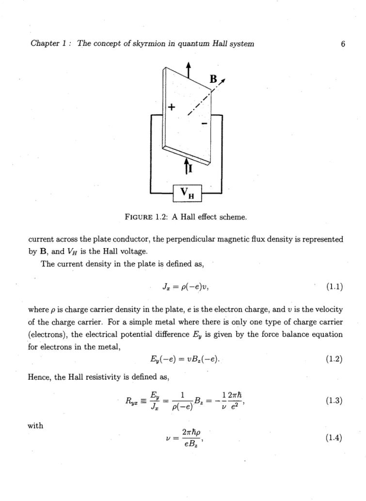
Now, we suppose that there is such a system as shown in Fig. 1.2 [13], where / is the

FIGURE 1.1: A to D represents four cases of Hall effect with different directions of mag-netic fields and electric current. In drawing "A", "1" represents electrons motion which is caused by an electronic potential difference "5" and has been bent by the magnetic field "4" induced by magnetic poles "3". The Hall effect takes on a negative charge at the top edge and a positive charge at the lower edge of the conducting medium "2" in "A". In "B" and "C", the polarization is reversed because of the reversal of the electric current or the magnetic field. For case "D", both current and magnetic field are reversed, which means the polarization is the same as "A".

Chapter 1 : The concept of skyrmion in quantum Hall system 6

FIGURE 1.2: A Hall effect scheme.

current across the plate conductor, the perpendicular magnetic flux density is represented by B , and VH is the Hall voltage.

The current density in the plate is defined as,

Jx = p(-e)v,- (1.1)

where p is charge carrier density in the plate, e is the electron charge, and v is the velocity of the charge carrier. For a simple metal where there is only one type of charge carrier (electrons), the electrical potential difference Ey is given by the force balance equation

for electrons in the metal,

Ey{-e) = vBz(-e). (1.2)

(1.3) Hence, the Hall resistivity is defined as,

*"* ' Jx ~ p(-e) z ~ with 2-irhp 12irh v e2 (1.4)

electrical devices use the Hall effect.

1.1.2 Quantum Hall Effect

In the former section, the relationship between Hall resistivity and magnetic field was linear. But if we restrict the conductor medium from 3-dimension (3D) to 2-dimension (2D) and, at the same time, increase the strength of the external magnetic field, we may observe a strange phenomenon, however, making us believe quantum theory more firmly. This unique phenomenon has been named quantum Hall effect (QHE).

The integer quantization of the Hall conductance was firstly predicted by Ando, Mat-sumoto, and Uemura in 1975 [14]. Then several works reported the observation of the ef-fect in inversion layers of metal-oxide-semiconductor field-efef-fect transistors (MOSFETs). It was in 1980 that Klaus von Klitzing, working with samples developed by Michael Pep-per and Gerhard Dorda, finally found the exactly quantized Hall conductivity [15]. For this contribution, von Klitzing was awarded the 1985 Nobel Prize in physics. After that, the fractional quantum Hall effect (FQHE) was discovered in stronger magnetic field in 1982 by D. Tsui, H. Stomer and A. C. Gossard [16]. Actually, the FQHE is beyond the scope of this report, so that we will not discuss it further.

Nowadays, integer quantum Hall experiments are performed mostly on GaAs-AlGaAs (gallium arsenide) heterostructures, and more recently in graphene. While a low temper-ature phenomenon in GaAs samples, the integer quantum Hall effect can now be observed in graphene at room temperature [17].

In a GaAs-AlGaAs heterostructure at low temperature, the electrons behave as a two-dimensional system. They are confined to the plane perpendicular to the interface

Chapter 1 : The concept of skyrmion in quantum Hall system 8

energies are given by (see Appendix A)

En = tw(n + -),n = 0,1,2,..., (1-6)

- = % (1.7)

m*

in which m* is the effective mass of the electron, and £ = A / % is defined as magnetic length. Hence, the energy of a 2DEG is not continuous under a perpendicular magnetic field, but the number of total quantum states should be the same as that without magnetic field, which means the degeneracy of Landau level is

S m*S eBS $

where ^ ^ is the density of states, and S is the area of the system. The quantum Hall resistivity is experimentally given by a set of plateaus at the exact value

Rxy = ±-Bz = ± = ^ . (1.9)

pe eln n

The resistivity is thus like a staircase as shown in Fig. 1.3. The constant RK = ^nr ~ 25812.807Q.

The physical meaning of the Landau-level filling factor (or filling factor for short) is,

Number of electrons p 2 Pe , >

Number of available states p$ hB There are many applications of quantum Hall effect in several branches of physics, for example, a measurement of the fine structure constant a.

1.2 Topological soliton: skyrmion and antiskyrmion

1.2.1 Soliton and solitary wave

One of the most interesting thing in physics is to study the excitations of a physical system. Interactions existing everywhere in our world may lead to various excitations. Sometimes, the excitation can be treated as a linear response to some perturbation exactly or approximatively. The linear response was thought to be sufficient in most

v = 6 5 4 3 2

Magnetic Field B±

FIGURE 1.3: Hall resistivity contrast between classical Hall effect and quantum Hall

effect. This picture is cited from [6].

parts of physics, but now, we have realized that nonlinear interaction is the real life, which may bring not only chaos, but also excitations that are called solitons or solitary waves, especially when the nonlinearity is weak. In fact a soliton arises in a nonlinear system when both the nonlinear interaction and the dispersion effect are considered, although either of the two may solely lead the collapse of the dynamical system. When both effects are present, the system may reorder to form a stable state, which means the two effects balance each other and a new order is brought by the combination of unstable elements.

Historically, the first observation of a solitary wave was made by a Scottish engineer, John Scott Russell, in August 1834. While he was walking along the Union Canal linking Edinburgh with Glasgow, he saw a rounded smooth well-defined heap of water separated from the prow of a barge brought to stop and proceed without any change of, shape or diminution of speed for over two miles, finally disappeared at the corner of the river. After his report, the research in nonlinearity and solitary wave in hydrodynamics and mathematics began.

In physics, the following definitions of soliton and solitary wave are given (the defini-tion is taken from [18]):

Chapter 1 : The concept of skyrmion in quantum Hall system 10

•i-m

•J-:- • •

t-FIGURE 1.4: Soliton in life, kink ice [19].

A solitary wave is a localized wave that propagates along one space direc-tion only, with undeformed shape.

A soliton is a large amplitude coherent pulse or very stable solitary wave, the exact solution of a wave equation, whose shape and speed are not altered by a collision with other solitary waves.

There are many kinds of solitons. The main types are:

(i) Bell-type soliton, like the solution of Korteweg-de Vries (KdV) equation

ut - 6u • ux + uxxx = 0, (1-11)

whose solution is

u(x,t) = -2n2sech2[K{x-AK2t-xQ)], (1.12)

XQ : constant, (1-13)

where 4K2 is the velocity of the wave.

(ii) Breather (envelope) soliton in nonlinear Schrodinger equation (NLSE)

Civ)

-4 0 4 -V

(iii)

4

4 $ X O

y\.

FIGURE 1.5: The collision of two solitons. whose solution is

u = 2r/sech[2r/(x - x0 - 4£t)] exp[2^x - 4i(£2 - rj2)t - i(j)0], (1.15)

?7, £,</>o : constant. (1-16)

(iii) Kink soliton, e.g. sine-Gordon equation (SGE)

iht — uxx + sin u = 0, whose solution is u v 4 arctan constant exp x — vt (1.17) (1.18) (1.19)

Soliton theory was first studied in hydrodynamics, but the concept of soliton is not limited to this branch of physics. After a few hundred years of development, many branches of physics borrowed the idea of soliton, e.g. optical solitons in optical fiber or other medium (multi-level system medium in optics) have been known for a long time and expected to be used in communications application for its unchanged shape transmission; bell-type (either dark or light soliton) solitons in Bose-Einstein condensation; kinks in

Chapter 1 : The concept of skyrmion in quantum Hall system 12 3.5 3 2.5 2 1.5 1 -10 0 10 20 30 40 50

FIGURE 1.6: A kink and an anti-kink.

Josephson transmission line, and soon.

The kink soliton has a special place in our report, not for its Lorentz invariance (of course, this point should be noticed), but because it is a topological soliton unlike the other two.

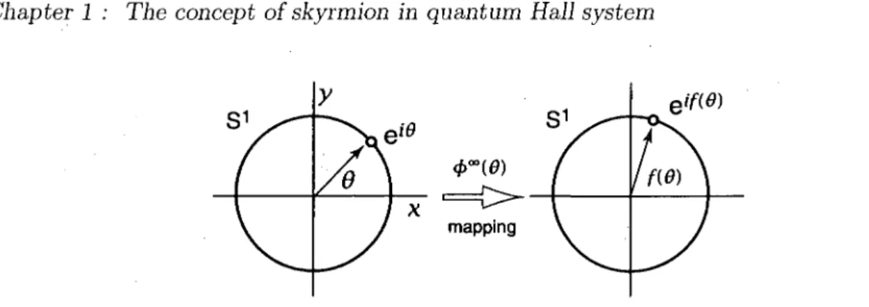
1.2.2 Topological soliton solution of t h e nonlinear sigma model

In order to review the concept of topological soliton, we need to review some mathematical knowledge about homotopy classes (see details and all mapping pictures of this section in Ref. [6]).

Let's begin with an example, a quantized vortex which can be generally written as a complex function,

(f){x)=ve-im, (1.20)

where 9 is the angle of the vector x with respect to the x axis in the xy plane. The density distribution of a vortex is like a Bell-type soliton.

Generally speaking, the hamiltonian of the system should contain the momentum term that is a second derivative of the field. To keep the energy finite asymptotically, we should demand the boundary condition of the vortex to be:

<TW = vo0e-iW\ (1.21)

FIGURE 1.7: (jf° defines the mapping from S1 to another S1. A point in the real space

(normal U(l) group) el6 is mapped to the point in velf^ in the field space uniquely by

(p°°. This is nontrivial.

e-«/(0) __• e-l90 ) the boundary condition is given by

<j>°°(9) = 0°°(x) = v^e -iq6 (1.22)

where q is an integer defining the vorticity of the vortex. If q ^ 0, the vortex is well defined (including the density and phase information) at all points only except at the origin. However, without loss of generalization, we can set

0(0) = 0. (1.23)

The boundary condition defines the asymptotical formula of the vortex, where the 6 6 [0, 2ir] with two endpoints identified. The boundary condition takes a value in the group space U(l) that is identified with a circle S1 because its element is written as e%*. It's not

surprising that both the boundary condition and vortex wave function take value from the U(l) group or S1 circle because the boundary condition gives a unique solution for a

differential equation. Hence, we can say that the boundary condition defines a mapping from U(l) group (the real S1 space) to the field space (another S1 space). The mapping

is illustrated in Fig. 1.7.

We have seen that the field space is grouped into topological sector eigd labeled by q.

The topological sector is called "homotopy classes".

In mathematics, we represent the above mapping (51 to another S1) by the set of

integers,

7r1(51) = Z. (1.24)

Chapter 1 : The concept of skyrmion in quantum Hall system 14

FIGURE 1.8: A mapping from U(l) (S1 circle) to a S2 sphere. The mapped circle in S2

is still a closed curved line that can be continuously shrunk to a point, which means the mapping is trivial.

space (from the left S1 to the right S1 in Fig. 1.7). In physics, the integer Z represents

the topological charge of a topological soliton.

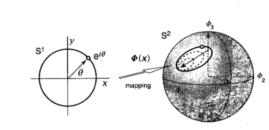
In Fig. 1.8, we show a mapping from S1 to S2, giving a trivial result that means the

homotopy class

7r!(52) = 0. (1.25)

In general, we have the following relationships in homotopy theory,

7r„(5") = Z, nn(Sm) = 0, for n< m, TiniS1) = 0, for n< 1. (1.26) (1.27) (1.28)

Homotopy groups irn(Sm) are not trivial (nonzero) when n ^ m. If the homotopy group

is not trivial, a topological soliton exists in the system. The quantized vortex is a fine example with 7Ti(S'1) ^ 0.

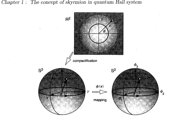
It is now time to introduce the topological solitons called skyrmion or antiskyrmion, which are present in the nonlinear sigma model. The Lagrangian of the O(N) nonlinear sigma model is defined as

Js

(d^) (d^), (1.29)

where Js is the spin stiffness, so that 0 is a TV-component dimensionless field and the

normalization condition gives

FIGURE 1.9: Firstly, compact the xOy plane (R2) to a S2 (in a 3D frame) sphere only

except the north pole where the boundary condition takes value. Then mapping from the

S2 to another S2 (a sphere based on 3 components of the field) is nontrivial, n2 {S2) ^ 0.

Here we use the Einstein's summation convention. Actually, the normalization condition gives the nonlinearity of the system. For simplification, we consider a 3-component field operator, <f> = (fa, fa, fa) defined in 2D. The finite energy condition

E = ^ fd2x(Wfa2 = ^ Uvcj) - fd2x(f>V2(t>

gives the boundary condition

lim V0 = 0, which implies the boundary condition,

lim far) = 0°°,

(1.31)

(1.32)

(1.33)

a constant.

Following the former discussion, the sigma field fax) can define a continuous mapping from the real space Sm to the operator field space 5'3~1. Since 7rm(S'2) ^ 0, there exists a topological soliton named skyrmion (or antiskyrmion). This discussion can be generalized

Chapter 1 : The concept of skyrmion in quantum Hall system 16 to N dimensions. In this case, the skyrmion, existing in the O(N) nonlinear sigma model, is called the C P ^- 1 skyrmion.

Next, we should define the topological charge. The following is still shown in the 0(3) model for simplicity. The 0(3) nonlinear sigma model Lagrangian may describe a spin-spin interaction model. In a planar geometry, a topological current is defined as

•^fcyto = ^^abctad^Mc, (1.34)

which is conserved trivially under the normalization condition,

V4,M = 0- (1-35)

Hence, it's easy to find the charge by integrating the first term of Jgky{x)

Qsky = / d2xJ°sky(x) = — / dPxeabceij<l>adi<i>bdj<l>c, (1.36)

which is defined as the topological charge.

We now give an example of the calculation of the topological charge. We choose the boundary conditions satisfying Eq. (1.30) and (1.33) as,

lim 0i(r) = lim <fe(r) = 0, (1.37)

r—»oo r—»oo

lim 03(r) = 1. (1.38)

r—>oo

Considering a spin or pseudospin polarized ground state, we can find a soliton solu-tion of the nonlinear sigma model (3D for simplicity) located at the origin in the polar coordinates,

2nqrq

& = ^ T ^

'

2Kgr9

*3 = pnj^f

'

>

with a positive q and K. Using this solution with the formula for topological charge, we find that

FIGURE 1.10: The arrows represent the vector field defined in Eq. (1.39) for the left

picture, and the Eq. (1.41) for the right one, respectively.

which is the topological charge of the skyrmion. The other solution is the antiskyrmion form

2Kqrq

^ = r2g + ^C O S( ^ ) >

r2q_K2q

^3 ~ r2q _|_ K2q '

which gives a topological charge Q = —q. Both types of soliton have the same energy

E = AnJs \Qsky\. (1.42)

This is the energy to make a spin texture at constant number of particles. In the next chapter, skyrmion and antiskyrmion will consist in adding or removing an electron from the system. In this case, they will have different energies.

The two vector fields of Eq. (1.39) and (1.41) are shown by the vector plots in Fig. 1.10. At the center of both pictures, vectors point straightly downward, while all vectors are polarized upward at infinity. The projection of vectors on the plane rotates (inversely in two pictures) by 2%, winding around the origin one time, which means the topological charge equals to 1.

In a quantum Hall system (2DEG), the spin textures can be described by the La-(1.41a) (1.41b) (1.41c)

Chapter 1 : The concept of skyrmion in quantum Hah system 18

grangian,

C = -±{d*S){d

S),

where S is the spin operator denned as

Si = X > « ^ * / » ' (1-44)

a,/3

SA = 1. (1.45)

Here \& is the field operator of the electrons and a is the Pauli matrix. According to the discussion of this section, it is possible to excite a soliton (skyrmion or antiskyrmion) of the spin field from the spin polarized ground state. The spin textures given by Eq. (1.39) and (1.41) are a perfect skyrmion and an antiskyrmion respectively. After considering Zeeman effect and Coulomb interaction, the shape of the solitons will change a little from that of Eq. (1.39) and (1.41). Due to the balance of the Zeeman coupling and Coulomb interaction, the state is still a soliton. More details of a physical system (2DEG in a quantum Hall sheet) will be giyen in Chapter 2.

In chapter 1, we have reviewed some knowledge concerning the quantum Hall effect and skyrmion. In the present chapter, we discuss the ground state and excitations of the 2DEG in a monolayer quantum Hall system. In the following content of this thesis, we will pay more attention to the spin and/or pseudo-spin texture in graphene. The reason why the spin textures are so important is that, under certain conditions that we will explain later, the spin textures are the lowest charged-energy excitations, i.e. they are the particles that carry the current [5,20]. We start this chapter by considering real spin textures which are easier to understand than the more abstract valley pseudospin textures.

The simplest excitation is an one-particle excitation, which means only one electron is removed from (or added to) the ground state. The system can be simplified to a couple of energy levels in a strong perpendicular magnetic field because of the Landau quantization (details are given in Appendix A). It is convenient to use the symmetric gauge

A = ^ B x r , 4 = ~By, Ay = \BX,AZ = 0, (2.1)

because we suppose that the excitation occurs in the center of the sample's plane and has a circular symmetry.

For the sake of simplicity, we only consider the case that the quantum Hall sheet is at filling factor v = 1, and energy gap between lowest and the first Landau level hwc

Chapter 2 : Single particle excitations in monolayer quantum Hall system 20

t? ~ % * t> <? %, •<?"% f ' \ e •%

- 1 0 — 5 c — G I — i ; — 5 J — 3 ;

m = 0 1 2 3 4 5

FIGURE 2.1: The spin generated ground state (Landau level n = 0) at filling factor */ = 1 is split by the external magnetic field B . The gap between two levels is the Zeeman bias A B = gfisB, where g is Lande factor and //# is the Bohr magneton. Each blue ball represents one electron at angular momentum m = 0 , 1 , 2 , . . . from left to right respectively.

is much bigger than the Zeeman bias (fou)c 3> g/J-sB). In this case, the Landau mixing

can be neglected. The ground state of the 2DEG at v = 1 is a ferromagnet even if

g = 01. That is because the ferromagnetic state minimizes the exchange interaction

energy of the 2DEG. The Hund's rule suggests that a gas of electron could lower its Coulomb interaction energy by maximizing its total spin. In a metal, this would lead to an increase in the kinetic energy of the electrons because of the Pauli principle. However, in the lowest Landau level, the kinetic energy is quenched by the magnetic field. Hence, electrons can completely fill one Landau level and all share the same spin orientation which we will take as directed along the +z direction [21].' The ground state of such a system can be written as

|G5) = n4,

,

|0), (2.2)

m = 0

where c1 is the creation operator for the lower level as shown in Fig. 2.1, m is the angular

momentum, and N^ is the degeneracy of the Landau level. Moreover, N^ is so big that it can be considered to approach infinity. In this chapter, we use oo instead of N^ in all these kinds of sums and products, and neglect the upper limit oo in all sum and product

F I G U R E 2.2: Quasi-hole state in the left picture and quasi-electron state in the right one. symbol, N6

£ - £ = £;

n - n - n

In this chapter, we only consider the excitation at Landau level n — 0. One electron is removed from the lower spin level or added to the upper spin level as shown in Fig. 2.2.

2.1 Hamiltonian of t h e system in t h e Hartree-Fock

approximation

The hamiltonian of the 2DEG must include the Coulomb interactions. We write it in second quantization He-e a \ E / / * * / * ! > ) * U r W r " rO*^(r')*n,Q(r), He_b = - jf dTdr'nh^nt0{r)^n^v)V{r-v% Hb-b = ^JJdrdr'nlVir-r'), (2.4) (2.5) (2.6) (2.7)

Chapter 2 : Single particle excitations in monolayer quantum Hall system 22

where ^n Q,(r) is the field operator of an electron in the nth Landau level with spin

a,fi = t or | , and rib = 2^2 > is the density of the positive charge of the background. In

the right side of Eq. (2.4), the first term is the Zeeman coupling, the second one He_e stands for the electron-electron Coulomb interaction, the third one He-b is the Coulomb

interaction between the electrons and the positive charge in the background, and the last one Hb-b represents the interaction between the positive charges in the background.

In fact, each Coulomb term in the right side of Eq. (2.4) is divergent. But once we sum over them (i.e. when we take into account the positive background), all divergent terms will cancel exactly. In order to cancel the divergence, we use the expansion

nb = 2n&

= J]K,m|

(2-8)

for the uniform background positive charge density rib, where <pn,m is the wave function

of an electron in the nth Landau level of the mth angular momentum.

In perturbation theory, the field operators can be expanded in terms of eigenstates of the non-perturbed hamiltonian that are obtained in Eq. (A. 17), i.e.

* n , a ( r ) = ^ Vn,m(r)Cn,m,a, ( 2 . 9 a )

m=—n

<

( r ) = £ <

(r)<

,

, (2.9b)

m=—n

where cn<rrita is the annihilation operator of an electron in the nth Landau level of angular

momentum m and spin a. We define cn,m^ = an>m and cn^m^ — bn^m. As we mentioned

before, only the lowest Landau level is considered (no Landau level mixing and no higher Landau levels). So we can keep n = 0 and drop the index n in all operators and functions. Then we put Eq. (2.9) into the hamiltonian of Eq. (2.4) and define the matrix elements

Vmiirn2,m3im4 = J drdrV5imi(rVo,m2(r)V(r - r>*m 3(r,)^o,m4(r')- (2.10) These matrix elements are called P j m m m in Appendix C. Then the hamiltonian can

m,m'=0

T ~ / y 'm,rn,m'm'•

m,m'=0

As in Eq. (2.4), the term in the first line of Eq. (2.11) is the Zeeman energy, the term in the second line is the electron-electron interaction, the term in the third line is the interaction between the electrons and the background positive charge and the last term in the fourth line is the constant energy of the background.

We consider the following states — one-particle excitation states:

M - = I I («-«m

i+^4)|0), (2.12)

m=0

|V)+ = n ( -u-a - - i+^ 6- )6o | 0 ) , (2.13) m = l

whose normalization condition ±{if>\ift)± = 1 gives

\um\2 + \vm\2 = l. (2.14)

If um,vm ^ 0, \ip)- corresponds to an antiskyrmion state and \ip)+ corresponds to a

skyrmion state. Otherwise, \ip)- represents a quasi-hole state and 1-0)+ represents a quasi-electron state.

In Eqs. (2.12) and (2.13) we introduced the quasi-particle operator {ua) + vtf) that is an operator combining electrons in two different spin states. In the mth quasi-particle,

|itm| represents the weight of a spin-up electron and |i>m| represents the weight of a spin-down electron. The (m ± l)th angular momentum electron in the spin-up state is combined with the mth angular momentum electron in the spin-down state if vm ^ 0. We

will see below, that these BCS-like pairs of electrons (as shown in Fig. 2.3) may decrease the energy of the system, because they permit to keep neighboring spins as parallel as

Chapter 2 : Single particle excitations in monolayer quantum Hall system 24

possible hence minimizing the exchange energy cost of an excitation. To compute the energy of the states |^}+ and IV7)-, we need

±{tl)\<4nam>\il>)± = Sm,m> |«m±i|2, (2.15)

±(tp\blnbm>\i))± = 5m,m>\vm\2, (2.16)

±{ip\alnbm>\ip)± = 6m±i)m>u*m±1vm>. (2.17)

We compute the energy of the states | ^ )+ and ^>)_ in the Hartree-Fock approximation (HFA). This HFA is obtained by approximating:

t t / t \ t _ / t \ t amiam2flm3ffim4 > \f lmiam4/am2 a™3 \amia«i31am,2a"mi '\am2a'm3)amiami ~ \am2am4)amia"m,3] % ! % ""sS — > \bm10mi)t>m20rn3 — \ 0m i0 m3) % % 4 + {hL2hm3)b]mJ)rn4-{b]m2bmi)b]mibm3 -am1bm2bm3am4 ~ * \am1a"mi)bm2Om3 — \ Qm i0 m3/ " m2 a m4 ' amiamAy)m2^31 ~ ami"m3\Om2Clm4).

The reason to do a Hartree-Fock approximation is that the Coulomb interaction in the hamiltonian of Eq. (2.11) is impossible to diagonalize or deal with exactly. Actually, the Hartree-Fock approximation is a mean-field method where the interaction between one electron and the other electrons is replaced by the interaction between one electron and the average field of all other electrons. In our case, the HFA gives good agreement between theory and experiment [5].

Finally, we obtain the effective HFA hamiltonian of the system,

H = -gtiBBY^(-aLam + blnbm)+^UH(m)(alnarn + blnbm)

m m -^(Ua(m)alam + UbF(m)blbm) m + Yl (Ui(m)blnam±l + h.C.) m + 0 A-^i Vrn,m,m',mi, (2.18) m,m'

m'

where U^ corresponds to antiskyrmion and f/f.fc corresponds to skyrmion, respectively. In the third line of Eq. 2.18, the lower limit of the sum is m = 0 when one electron is removed (we get Uf), and m = 1 when one electron is added (we get Uik), respectively.

When averaging the hamiltonian, terms like ( Y2iam'arn'}amarn ) should not be counted

twice. This means that /Y^(aL'am')'4nam) —> i E (aLf lm ' ) (aLam ) ^ Hence, the energy of the states \I/J)± are

E± = (H) = -

-^-J2((

^m)-(blb

))

+ E ^

Wmx^i) , (bmibmi)

((alam) + (blb

))

^ / j Vm,mi,mi,m \\amiami) \amUm) + \bmibmi) \bmbm/)

m,mi

~ / j ^ m , m i , m i ± l , m ± l ( flmi±l"mi ) \ V m ± l / + ^ / J •'m.m.mi.mi • \l.2X))

m,m\ m,m\

2.2 Quasi-hole and quasi-particle states

The simplest one-particle excitation states are shown in Fig. 2.2. They are called the quasi-hole and quasi-electron states, i.e. one electron is removed or added to the sys-tem. The energy to create a hole-electron pair can be calculated analytically and be measured directly in experiments. It is important to compare the excitation energies of quasi-particle and spin textures, so that we can decide which state is the lowest charged excitation and justify the theory.

Firstly, the energy of the ground state is the average of the hamiltonian on the ground state \GS) — Y[ a-lnl®)- ^n ^m s c a s e' it's e a sy t ° find U± = 0, (b^bm) = 0 and (aj^a™) = 1.

Chapter 2 : Single particle excitations in monolayer quantum Hall system 26

The hamiltonian of the ground state can be simplified to

m m,m'

2

m,m' m,m'

Hence, the ground state energy is

j ^ 1 ^

EGS = {H)GS = ~-^9^BB 2_^ 1 — ^ 2 ^ Vm,m',m,',m, ( 2 . 2 2 )

m=Q m,m'=0

where N<p is the degeneracy of the Landau level n = 0. In the final formula of the ground state energy, there are only two terms, one is the Zeeman energy and the other one is the Fock (exchange) energy. All Hartree energies ( electron-electron Hartree interaction and electron-background Hartree interaction) cancel exactly.

For the quasi-hole state (shown in the left picture of Fig. 2.2), \h) = Y[m=i am|0)> i-e -there is one electron missing in the m = 0 angular momentum of the 2DEG. Thus, the excitation energy of the hole state is

N$ -. N4> N4>

Eh = (H)h = —-^gflBB y j 1 + ^ 2_j Vm,m,m',m' — 2_j Vm,m,m>,m'

m = l m , m ' = l m = l , m ' = 0

7) / j ' m , m ' , m ' , m i~ 7> / J ^m,m,m',m'i \Z.Zo)

m , m ' = l m , m ' = 0

because (a],ao)/i = 0. Using the fact that Vm,m,m\m' = Ki',m',m,m and Knim',m',m =

Vm',m,m,m', W e g e t

iV0 . N<t> ' N<t>

Eh = (H)h = —-gUsB 2_^ 1 ~ « 2^i ^rn,m',m',m + /_^ ^ 0 , m , m , 0 - ( 2 . 2 4 ) m=l m,m'=0 ro=0

We find that the energy needed to excite one hole is

1 "<t> •, j — 2

AEh = Eh - EGS = -~gfiBB + ] P Vr0,m,n.,o. = -^9^3 + v / ^ ^ »

m = 0 *

Ee = (H)p = ~gfiBB^l + ^gfjiBB-^ ^ Vm,m>,m>,m. (2.26)

m=0 m,m'=0

In the similar way, we obtain the energy to add one electron to the 2DEG,

AEe = Ee- EGS = ^gfiBB, (2.27)

which is only the Zeeman energy of the added electron. It's easy to explain such a simple result: the added electron is placed in the spin-down level. The Hartree energy between the new electron and other electrons in the spin-up level cancel the energy due to the interaction between the background positive charge, and there is no exchange (Fock) energy between electrons of different spins.

Combining our two results, we find that the ferromagnetic liquid state at v = 1 has a transport gap given by

AE

= AE

+ AE

= ^ 1 (j^j , (2.28)

if spin texture states are not considered. This gap can be found experimentally by measuring the temperature dependence of the resistivity pxx ~ e-Aeh/(2fcsT) in the QHE [21].

2.3 Spin textures

In section 2.2 we discussed one type of excitation of the ferromagnetic state at u = 1. We may consider another way to excite the system which involves spin textures.

Chapter 2 : Single particle excitations in monolayer quantum Hall system 28

—O-O-O-Q-O—

FIGURE 2.3: The upper picture sketches the antiskyrmion state (Eq. 2.12) where a0 is

removed. And the lower one represents the skyrmion state (Eq. 2.13), the blue dot is the added electron b0. The BCS-like pairs are formed in spin texture states.

state at v = 1 can be written as

C = ^g»BBASz - ^ (&>S) (dpS) + C (S, S'), (2.29)

with the normalization condition

\S\2 = 1, (2.30)

where ASZ is the spin difference from the ground state, C(S, S') is the Coulomb energy

due to the change in density, and Js is the spin stiffness which is related to the cost in

exchange energy when the spins are no longer parallel.

The field-theoretical approach is good for a smooth field, i.e. the excitations are not too localized (large skyrmions). In order to consider the spin textures of all possible sizes, we will solve our problem not with Lagrangian, but with the microscopic hamiltonian of Eq. (2.18) using a canonical transformation (discussed in Appendix B). We use the hamiltonian and the spin texture states of Eqs. (2.12) and (2.13) derived in section 2.1. In this case, each spin-up electron with mth angular momentum is paired to the spin-down one with (m ± l)th angular momentum (as shown in Fig. 2.3), so that the projection of spin polarization on the xOy plane rotates by 1-K along any path winding around the origin one time.

In each pair, there is only one charge or one electron. The electron has a probability |ttm|2 to be in the mth angular momentum of spin-up level and a probability |fm|2 to be

According to Appendix B and Eq. (B.8), we choose um and vm to be real numbers

without loss of generality. Then, the energy is a function of um and vm:

EV \ 9^BB ST^ / 2 2 \ , V ^ T / fUm1~l . Vmi , \ 2 E(Um,Vm) = — 2_^ ( V l -Vm)+ } _ ^ Ki.m.mi.rm [ ~ ^ ~ + ~y ~ l J Um-1 m ra,rai 4 . V V fUm1-l + V _ l V / _ l V l / (v2 V2 +V2 V2) ' / J vm,m,m1,mi I n ^ 9 J um r, / j vm,mi,mi,m \u m i- lum - l ~ umium) m,mi ^ m,m\

/ j Vm,mi,m^ + \,m+l'^m\'VrniUmVrn + — y ^ ' m , m , m i , m r \£.ol)

2

mi m,m\

We write the energy functional with Lagrangian multipliers \m to include the constraint

due to the normalization condition of Eq. (2.14)

F(um,Vm,Xm) = E(um,Vm) + J2Xrn{Um+Vm-1)- (2- 3 2 )

m

To minimize the functional, we compute

- = 2X

+ 2[-G-J2

"n = "^i^i "T ^ I CJ- y j 'i,i,m,m I fy i " / _, \ ' m,m,i,i *i,m,m,i) VmVi

1 \ m / m=0

dF_ dui

+ 2 ^ Vi^m+hm+iU2mVi - 2 Y^ Vi,m,m+l,i+lUmUiVm = 0, ( 2 . 3 4 )

m=0 m=0

Chapter 2 : Single particle excitations in monolayer quantum Hall system 30

where G = \g^BB.

Equation (2.35) is the normalization condition. Taking Eq. (2.33) xt>j — Eq. (2.34) xitj, we find I G — 2_^ Vii,m,m I ~ I —G — 2_^ ^ i + l . i + l . m . m I UiVi (2.36)

+

+

£"«

S>

which does agree with the main equation (B.3) given by canonical transformation con-dition, the nondiagonal elements being zero. Hence, the two methods give the same self-consistent equations of um and vm as those shown in Eq. (B.7). In fact, there is a

trivial solution um = l,vm = 0 that is the solution of quasi-hole state, but it does not

minimize the energy state (we will see this below). Now, we describe the system in the spin language,

Si = X > ^ * *

5 ± = ~ 2 ~ ~ ' where a1 is the i-th. component of Pauli matrix,

(2.37)

(2.38)

ax =

1 0 / I % 0 / I 0 - 1 (2.39)

We submit the expansions of the field operators, Eq. (2.9), into the spin operators, so that,

S

(r) = £ ( k ( r V

y(

) = Y, ( - ^ (

) ^ ' (

)

i ^ + < ' ( r ) ^ ( r ) t « m )

(2.40b)

1 . , • i % 1 t ' . . . i . / / • , 1 1 - 4 - 2 0 2 4 - 4 - 2 0 2 4

FIGURE 2.4: Density and spin texture of an antiskyrmion. The pictures of this numerical experiment is done under Zeeman bias ^ / X B S / 2 = 0.01, in which all lengths are in units of I and energies are in units of ^ . In all of these numerical computation, only the parameter of Zeeman bias is tunable.

If there is no spin texture i.e. only quasi-particle states are excited, the average value of those operators (2.40) will be trivial (zero). If the average of spin operators are non-trivial, as we mentioned before, there might exist topological soliton minimizing the energy of the system, i.e. antiskyrmion state or skyrmion state. The topological soliton existing as spin texture may decrease the energy compared to quasi-particle state that is a spin polarized state.

After numerically calculating the set of self-consistent equations (B.7). We get a set of um and vm that gives all information about the spin texture states including average

value of spin operator and total energy of the excited state. Furthermore, a real-space graph of the spin texture can be made, as well. Strictly speaking, the spin texture that we get is not an exact skyrmion or antiskyrmion, because the Lagrangian Eq. (2.29) contains the Coulomb and Zeeman couplings, in addition to the gradient term.

It is important to compare the excitation energy of quasi-particle states and spin texturs in order to decide which type of particle will be excited at v = 1. The energies of spin textures can be only obtained numerically.

In Figs. 2.4, 2.5, patterns of spin textures are shown. Firstly, we indicate the anti-skyrmion state where the direction of the spins rotate in a clockwise direction.

Secondly, the skyrmion state is shown, where the spins rotate in the anticlockwise direction.

Chapter 2 : Single particle excitations in monolayer quantum Hall system 32

FIGURE 2.5: Spin texture of skyrmion. All conditions and units are the same as those shown in the case of antiskyrmion in Fig. 2.4.

The size of a skyrmion is the result of a competition between the Zeeman term that opposes spin-flip and favors small skyrmion and the Coulomb energy in the density profile which favors large skyrmion. The spin texture has a large-size if the Zeeman effect vanishes. Conversely, the spin texture collapse to the quasi-particle state if the Zeeman term is large enough.

Finally, we give in Fig. 2.6 the excitation energies of skyrmion and quasi-particle states. We find that the spin texture excitation costs less energy than quasi-electron state at small Zeeman couplings. Hence, the spin texture excitations are the lowest single particle excitation states in such a system instead of quasi-particle state, at low Zeeman energy.

The Zeeman energy can be tuned independently of the magnetic field by straining the sample. This has the effect of modifying the g factor by strain force. Once the Zeeman gap is tuned to be larger than a critical value, the quasi-particle states will occupy the lowest excitation state instead of spin texture's states. That is because the strong Zeeman coupling destroys the spin texture. In our system, we find that the critical value for the transition to quasi-particle excitation is gnsB/2 ~ 0.04(e2//^).

The results that we got in this chapter were first obtained in Ref. [5]. We reproduced them here in order to explain the calculations that need to be done to compute the energy of a spin texture. We will use the same approach in Chapter 4 to compute for the first time the energy of skyrmions in graphene bilayer.

2 "o x UJ 1 0.95 -0.9, quasihole antlskyrmion 0.005 0.01 0.015 gnBB/2 0.02 0.005 0.01 0.015 9HBB/2 0.02

F I G U R E 2.6: Excitation energy comparison between quasi-electron states and spin tex-tures at different Zeeman bias.

1.4 1.3 1.2 1.1 1 10.9 0.8 0.7 0.6 P J i i L - • quasi-particle pair - • skyrmion anti-skyrmion pair

0.005 0.01

9HBB (e2/kl)

0.015 0.02

FIGURE 2.7: The energy comparison between two kinds of single-particle excitations at small Zeeman couplings. The red line represents the energy Aeh to excite a quasi-hole and

quasi-particle pair (given in Eq. (2.28)), while the green curve is the energy (computed numerically) to excite a skyrmion-antiskyrmion pair.

Chapter 3

Quantum Hall crystal phases in

monolayer graphene

Graphite is a very common material in our life, it is also made of the most common atom on earth i.e. carbon. Although some carbon-based materials have been studied for thousands of years, new allotropes have been found recently such as buckyballs and car-bon nanotubes besides diamond and graphite that were discovered long ago. Graphene, another allotrope of carbon, is a single layer of graphite.

Our goal in this chapter is to look for ground states of the 2DEG in graphene in the form of crystal of skyrmions with both spin and valley pseudospin textures. Skyrme crystal phases have been already studied by Cote et al. [9], but they considered only valley pseudospin textures and assumed that spin were completely polarized. In this chapter we want to see if it is possible to admix some amount of real spin texture in the valley pseudospin texture.

We first start by explaining the properties of graphene and in particular the energy spectrum of the 2DEG in graphene in the presence of a perpendicular magnetic field. Then we find out the liquid phases at filling factors v = 1,2,3,4. Finally, we discuss some unusual electronic properties and crystal states such as Wigner and Meron crystals in graphene by numerically solving the equation of motion for the single particle Green's function.

been observed in experiments save the stability of the single layer crystal, because the bending sheet makes the system embedded into the third dimension. Thus, a rippled graphene sheet can be stable at finite temperature.

Another interesting effect observed recently in graphene is the room temperature quantum Hall effect [17]. In semiconductor 2DEG, it can only be observed at very low temperature. In fact, much evidence supports that graphene is a special quantum Hall material in comparison with other 2DEG systems such as GaAs-AlGaAs heterojunctions, MOSFET, etc.. For the normal quantum Hall materials, there is 2-fold degeneracy in each Landau level due to spin. In graphene there is a 4-fold degeneracy of each Landau level. That is because the honeycomb first Brillouin zone has two kinds of inequivalent valleys K and K' as shown below. This extra degeneracy leads to much richer physics as we will see.

3.1.1 Crystal structure

Now, we study in detail why graphene has so many interesting properties. Let's begin with the geometry of this crystal.

Graphene is a 2D honeycomb lattice as shown in Fig. 3.1. There are two C atoms per unit cells. The crystal structure can be represented by two basis vectors a i and a2 in the plane xOy, and has a triangular Bravais lattice. There are two carbon atoms in each unit cell, which we denote by A (red dots) and B (the blue dots) in Fig. 3.1. We choose atoms A as our triangular lattice whose basis vectors are

(3.1a)

a2 = ' a (1,0), (3.1b)

where a = \/3c, c = 1.42A, and c is the distance between two nearest neighbor atoms.

V3

Chapter 3 : Quantum Hall crystal phases in monolayer graphene 36

F I G U R E 3.1: Graphene crystal lattice. Each red atom is linked to its three nearest neighbors by vectors <$i, 62,63. The C atoms can be separated into two kinds of atoms denoted by red (A) and blue (B) dots, i.e. we can divide the whole lattice into two sublattice whose lattice vectors are a i and a i .

We can move one red atom (^4 atom) to any point in the A-sublattice by the translation vector R = n i a i + n2a2. Hence, the reciprocal lattice vectors are given by

2?r , n

b2 =

(3.2a)

(3.2b)

which is also a regular hexagonal lattice as shown in Fig. 3.2.

The three nearest blue neighbor atoms of one red dot are separated by

51

=

(ir>\)

(i^3j>

h = c(0,-l) = o ( 0 , ~ V

FIGURE 3.2: Reciprocal lattice based on {bi, b2J and the first Brillouin zone represented by the red regular hexagon.

The first Brillouin zone that is the smaller regular hexagon plotted in Fig. 3.2. In the first Brillouin zone, there are two inequivalent points respectively, K and K'. Each

K or K' point can be translated to other equivalent K or K' by a combination of the

two basis vectors of the reciprocal lattice. We choose

K K' 2TT a [~3 2v (2 ,0 a ,0 (3.4a) (3.4b)

3.2 Band structure

Each C atom has 4 valence electrons. In graphene, three electrons bind covalently with the three nearest neighbor C atoms. The last valence electron, in the pz orbital, is

responsible for the conductivity of graphene. In the simplest model, we only consider the hopping of electrons between nearest neighbor atoms in the tight binding approximation. In this case, we can write the tight-binding hamiltonian as

H = - t ^ (a\bj + h.c.^ , (3.5)

Chapter 3 : Quantum Hall crystal phases in monolayer graphene 38

where t RJ 2.8 eV is the coupling constant between the two nearest neighbor C atoms in the pz orbital. The value of the second and third nearest neighbors coupling parameters

are 0.1 eV and 0.07 eV, respectively, which is very small in comparison with the nearest neighbor coupling so that the tight binding approximation with the nearest neighbors only is a good approximation. The symbol a; denotes the annihilation operator of electron on a red atom at position i and bj denotes the annihilation operator of electron on a blue atom at position j . Actually, a and b are fermion operators so that they satisfy the commutation relation,

|cJ,d,-J = SCid5ij, (3.6)

all others = 0, (3.7)

where c and d represent a or b. To analyse the system easily, we define the Fourier transformation of a and b:

where N is the total number of crystal sites, c^ is the annihilation operator in momentum space, R e represents R A for c = a, and R B for c = b. We have

{Ck'Ck'j = <Vk', (3 9)

all others = 0. (3.10)

By Fourier transformation, the tight binding hamiltonian can be written as

R S . k (5

- ? u * ) U °

w A

o

w

) ( ; ) ; ™

E+(k) = + x/A(k)A*(k), 1 N/2 E_(k) = - V A ( k ) A * ( k ) , i v/2 Hence, we obtain D^ E+ 0 0 E_

u= v W v^i

With the canonical transformation and quasi-particle operators cMik and c„k

(3.14)

(3.15)

(3.16)

c+k

=W T

\u,

C-,k / V »k

we can diagonalize the tight binding hamiltonian to obtain

H = J2E+

(

)

+,kC+*+E ^- (

)

-,k

-*'

(3.17)

(3,18)

with

A(k) = - * ] > > * • ' = - t ( ef a( *+& ) + c* ( - * + & ) + e - i a ^ ,

the energy bands are given by

E(k) = ±y/\MVf = ±t

\

(3.19)

Chapter 3 : Quantum Hall crystal phases in monolayer graphene 40

FIGURE 3.3: Energy band or dispersion relation and the Dirac's cone.

These dispersions relations are shown in Fig. 3.3. The Fermi level for pure graphene is at the vertex of the Dirac's cone. The valence band is filled by electrons while the conduction band is filled by holes.

Now, we consider the dispersions only around the K and K' points in momentum space where the band structure shown in Fig. 3.3 is almost linear in momentum k. We call the 6 cones at K and K' points the Dirac's cones because the dispersion relation near K and K' is that of a relativistic E = y/pPc2 + mlc4 —> pc massless particle. By the definition of Eq. (3.4), the dispersion around K points is

E(K + p) « ± ^ | p | o , ( | p | « | K | ) , (3.21) by Taylor expansion. In a similar way, we find the same result around the K' points

£(K' + p)*±f*|p|a, |p|«|K'|.

The group velocity at points K or K' is given by

1 dE \/3

VF =

MP7

m^

It is about 1 x 106 m/s, i.e. 300 times smaller than the velocity of light. We can write

the energy in terms of up and | p | as E(p) =

±hvp\p\-Due to the geometric structure of graphene, the electronic dispersion relation is linear near each valley in the first Brillouin zone. In these regions, we must use the Dirac

Firstly, we analyse the wavefunction around the K point:

A(K + k) = -tJ2e

'

5

= -t^ik-SJ™, (3.24) 5

because Yls e%K & = ®- Using the definitions of Eq. (3.3) and the vectors K and K', we

find

A(K + p) = -y-at(px-ipy), (3.25a)

A(K' + p) = + - y a t ipx + ipy). (3.25b)

Around points K and K', we thus have the matrices

^ • ^ - ( V - T J - ^ U T ' -

(3

-

26b)

where 9 = arctan —. Hence, the total Hilbert space of the system is K 0 K ' .

For the isolated K and K' valleys, the eigenfunctions are two-component spinors in the basis {\A, K), \B, K), } and {\A, K'), \B, K')} respectively, where |-4) = I J and