Building Local Maps for Robust Visual Navigation
by
Jeremy
S. Gerstle
Submitted to the Department of Electrical Engineering and Computer
Science
in partial fulfillment of the requirements for the degree of
Master of Engineering in Electrical Engineering and Computer Science
at the
MASSACHUSETTS INSTITUTE OF TECHNOLOGY
February 2001
©
Jeremy S. Gerstle, MMI. All rights reserved.
The author hereby grants to MIT permission to reproduce and
distribute publicly paper and electronic copies of this thesis document
in whole or in part.
Author...
Depw4rment of'/lectrical Engineering and Computer Science February 8, 2001
Certified by..
W.
Leslie P. Kaelbling
Professor of Computer Science and Electrical Engineering
Thesis Supervisor
Accepted by...
...
Arthur C. Smith
Chairman, Department Committee on Graduate Students
MASSACUSETT 1 S
OF TECHNOLOGY
JUL 1 1 2001 BARKFR
LIBRARIES
Building Local Maps for Robust Visual Navigation
by
Jeremy S. Gerstle
Submitted to the Department of Electrical Engineering and Computer Science on February 8, 2001, in partial fulfillment of the
requirements for the degree of
Master of Engineering in Electrical Engineering and Computer Science
Abstract
This thesis describes a robust low-level visual navigation system used to drive Erik, an RWI B21r, robot around cluttered labrooms as well as spacious hallway corridors and playrooms of the Al lab. The system achieves robust navigation of office-like environ-ments in the presence of partially unmodelled noise by combining simple and efficient visual processing, fast mapping and a near-optimal anytime planning algorithm. It is intended to demonstrate that sophisticated near-optimal navigation strategies can be found using fast integration of highly dense approximate visual and odometric data into small, temporary room-sized maps. The navigation algorithm follows from recent research on embedded learning agents and the theory of stochastic optimal control, and can be used as a framework for integrating multiple sources of information into coherent room-level navigation policies. The system is also fairly robust to modest but constrained changes in a number of its internal parameters. In this thesis, I will give an overview of the system's construction, describing the theory behind the inner workings of each subsystem, and analyzing the validity of simplifying assumptions in the context of the robot's operating environment. I will then conclude with the re-sults of several test runs illustrating overall system functionality, and discuss possible improvements that can be made in the future.
Thesis Supervisor: Leslie P. Kaelbling
Acknowledgments
A number of people have lent me their expertise, wisdom, and support throughout
my days at MIT and especially while working on this thesis. First, I would like to thank the entire Learning in Intelligent Systems lab, especially my advisor Professor Leslie Kaelbling for her consistent and helpful insight, extraordinary patience, and for being a true mentor; showing me how to be methodical, critical, unceasing in my pursuit for results, and unwilling to throw in the towel and claim defeat. A special thanks to Bill Smart who taught me the difference between good and bad C/C++ programming technique, for writing SeRF without which I would never have gotten off the ground, and for providing nearly round the clock technical support. Also, a special thanks to Terran Lane for spending significant time helping me understand and improve my algorithm. I would also like to thank Selim Temizer for his helpful insight and hours of code debugging help, along with Kurt Steinkraus for lending me his tcp/ip networking classes without which I might have spent unnecessary time struggling to write my own. Outside of LIS I would also like to thank Phd Sandy Wells for his help with understanding the math of camera calibration, and Polina Golland along those same lines for giving me the idea for camera tilt parameterization and hours of help developing the math to support it. While there are a number of other people in the Al lab that have helped me with this M.Eng thesis, I would like to give a special acknowledgement and thank you to PhD student Michael Wessler who first introduced me to world of reinforcement learning, taught me how to analyze and understand its mathematics, and without whom I might not have had an M.Eng thesis. Additionally, I would like to thank my friend Dan Zelazo for his support and constructive critiques throughout the research process. Romy Nakagawa and Rania Khalaf, and the rest of my friend at MIT for making me take breaks when I thought
I was going to lose my head. And finally, an all important thank you to my family. I am grateful for your unceasing support and love. Especially to my brother Ari for
taking on the undesirable task of helping me proof read and correct this paper in its final hours.
Contents
1 Introduction
1.1 Architecture : System Overview . . . . 2 Obstacle Detector
2.1 Theoretical Overview . . . . 2.1.1 The Ground Plane Constraint . . . . 2.1.2 The Background Texture Constraint . . . . 2.2 Design and Construction . . . . 2.2.1 Edge Detection . . . . 2.2.2 Using the Obstacle Detector for Reactive Control
2.3 Subsystem Analysis . . . .
3 Depth Recovery
3.1 Perspective Projection Camera Model . . . .
3.1.1 Perspective Transform : Affine Equations . . . . .
3.1.2 Projective Geometry . . . .
3.2 Camera Calibration . . . .
3.3 Recovering Floor Coordinates . . . .
4 Occupancy Grid Map
4.1 Constructing Occupancy Grids . . . .
4.1.1 Background on Use and Application to Vision . . . . 4.1.2 Integrating Occupancy Evidence . . . .
9 12 15 . . . . 15 . . . . 16 . . . . 16 . . . . 19 . . . . 19 . . . . 20 . . . . 22 24 . . . . 24 . . . . 25 . . . . 27 . . . . 28 . . . . 30 35 35 36 37
5 Navigation : The Planning Module
5.1 The Agent-Environment Feedback Model ...
5.1.1 Overview of Markov Decision Processes . . . .
5.1.2 Sidebar : On the Applicability of the MDP Framework
5.1.3 Solving finite MDPs . . . .
5.2 Value Iteration and Planning Algorithm . . . .
5.2.1 Stopping Criteria : Planning Time verse Control Time
5.2.2 Incorporating Proprioceptive Knowledge . . . .
5.2.3 Optimal Behavior : Exploitation verse Exploration . .
6 Actuator Control
6.1 Base Actuation . . . .
6.2 Pan-Tilt Actuation . . . .
7 Results
7.1 System Analysis . . . .
7.1.1 The Problem with Camera Tilt . . . .
7.1.2 Map Size Parameters . . . .
7.1.3 Probability and Certainty Parameters . . . .
7.2 Conclusion and Future Work . . . .
A Calibration Code 43 . . . . 43 . . . . 45 . . . . 47 . . . . 52 . . . . 54 . . . . 54 57 . . . . 59 61 61 62 64 64 65 67 69 70 72
List of Figures
1-1 The Navigation Task : Local Signposts give global information . . . . 9
1-2 Block Diagram of System Interactions. . . . . 12
2-1 The Ground Plane Constraint . . . . 17
2-2 Processing an Image into a Radial Depth Map . . . . 18
2-3 Comparison of Edge Detectors : detector used by Erik picks up the legs of the table but also more shadows. . . . . 20
2-4 Partitions of the Radial Depth Map : 1(t), r(t), c(t) marked. ... 21
3-1 Perspective Projection Camera Model . . . . 25
3-2 Calibration Pattern : Black tape reference points, and red circles show their calculated reprojection. . . . . 29
3-3 Recovery of Floor Coordinates : World coordinate system rigidly at-tached to the floor. . . . . 32
3-4 Accuracy of Floor Coordinate Recovery . . . . 33
4-1 RDM gives grid cell occupancy information. . . . . 38
4-2 Evolution of an Occupancy Grid . . . . 42
5-1 The Agent-Environment Feedback Model . . . . 43
5-2 Planning Algorithm Employed on Erik . . . . 48
5-3 Evolving belief state : cooler colors indicate lower map occupancy, and lower total expected cost to goal in the corresponding plan. . . . . 50
5-4 The value function and policy mature with time and exploration. The maps on the left are occupancy grids with stable wall obstacles clearly defining the boundary of the explored space. The associated value function which it generates is to its right. . . . . 58 5-5 The Modified Transition Function : Erik's diameter is three grid cells
in length . . . . . 59
7-1 Obstacle Detector fails leading to imminent collision. . . . . 66
List of Tables
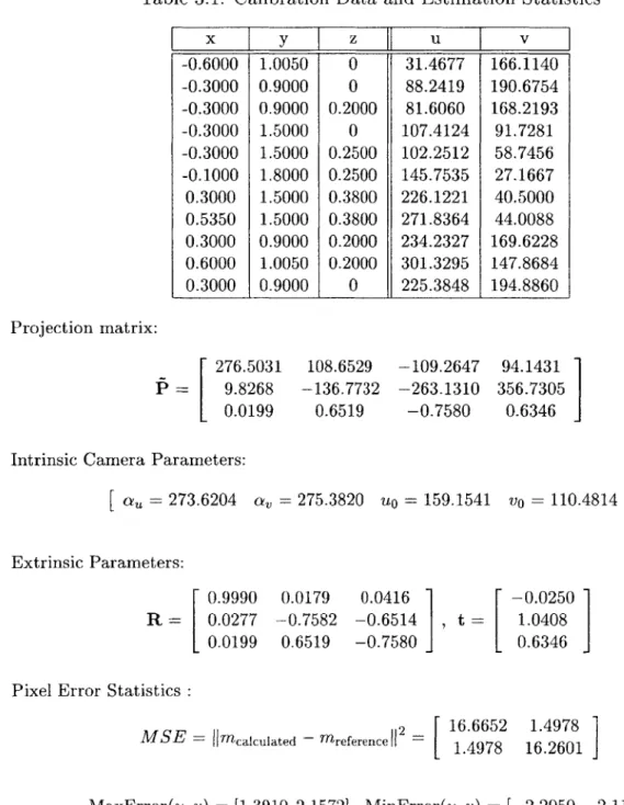
3.1 Calibration Data and Estimation Statistics . . . . 31
Chapter 1
Introduction
Rm916 by heaing alon tis Path 0? 1?btFigure 1-1: The Navigation Task : Local Signposts give global information
Suppose you blind-folded a person, dragged him or her to room 916 of the Al lab, took off their blindfold and told them to go to the conference room at the end of the hallway (presuming they've never even been in the Al lab before). Assuming they understand what a hallway is, and can read the label on the door of the conference room, the task is trivial: leave room 916, walk straight down the hallway, and near the end look for the conference room door. However, suppose the hallway is blocked
person would probably still be able to find his way by finding a door opening to the hallway on the other side of the building which also connects to the conference room. Finding the door and piecing together how rooms connect is the process of forming a topological map, a graph of landmarks (nodes) connected by rooms and corridors (edges). Navigating within rooms and corridors to discover passable ways of getting to known landmarks requires avoiding obstacles and methods for getting to the each "signpost". A mobile robot that can navigate rooms and corridors well without getting stuck in local minima will stand a better chance of discovering new landmarks and eventually knowledge of the underlying graph structure. The construction of a framework for learning robust visual navigation policies for robots in an office building environment therefore begins with a low-level navigator that can recognize obstacles and avoid getting stuck in local minima. This is the impetus for the system built in this thesis.
The inspiration for building the navigation system described in this thesis came from Ian Horswill's work on Polly, a vision based mobile robot that could give tours of the 7th floor of the Al lab. Polly used simple visual machinery and purely reactive control processes in a subsumption like architecture[2] to achieve its navigation tasks. While its simple machinery required very little computational power, the overall ef-ficiency of the controller was due to the specialization of each of its subsystems to its task and environment. The ability of each subsystem to perform its given task was therefore highly dependent on the degree to which idealized assumptions made
by the specialized subsystem matched a given environment. Polly could easily
re-cover from errors in its high level navigation modules due to their interdependent interaction with the environment. If the robot got confused or lost, it could wander around relying on its obstacle avoidance routine to keep it from bumping into things until its place recognition system triggered on something that would re-localize it. The robot's recovery was therefore dependent on its embedding in the environment, it had no method for replanning: changing its path intelligently once its current plan failed.
By keeping track of where obstacles are in the world a robot can account for
errors in perception and can recover quickly from failure in its high-level navigation subsystems by replanning. This is the formula for the navigation system described in this thesis. Gathering local information into a global occupancy grid data structure, Erik our RWI B21r robot, captures a cumulative history of what it has seen, and continously replans given its current state of information.
Figure 1-2: Block Diagram of System Interactions.
1.1
Architecture : System Overview
The navigation system consists of five subsystems:
* Obstacle Detector - produces immediate information describing where obstacles
are in the robot's visual field relative to its base.
* Depth Recovery - converts local image pixel data into global map coordinates.
* Occupancy Grid Map - integrates obstacle detector data over time to construct
a map of the probability of occupancy at discretized locations in the global or world coordinate frame.
* Path Planner - combines information from the occupancy grid and robot
odom-etry instructing the robot which immediate control actions to take.
* Actuator Control - applies the appropriate control to execute the path planner's instructions, and checks overall system sanity, possibly overriding the planner's instructions when needed.
Each of these subsystems is built to work in a modular fashion such that any one subsystem can be swapped out and replaced by another bearing the same input-output relationship and satisfying a basic set of constraints. Figure 1.2 illustrates the overall system processing.
The Obstacle Detector used is borrowed from Ian Horswill's work on low-level visual collision avoidance for mobile robot navigation. The detector takes as input a video stream from the robot and produces a radial depth map, a description of relative distance along the floor from the robot's center to obstacles in its field of view that project up significantly from the ground plane. Details of the detector's functionality are described in chapter 2. It is worth mentioning here that this particular choice of detector has led to certain overall system design considerations which might be dispensed with given another choice of obstacle detector. The detector makes a reasonable assumption about the robot's operating environment, namely that the floor in an office environment is is textureless at a large scale. This assumption imposes certain constraints which may impact the reliability of the occupancy grid and path planning subsystems if violated. Other detectors, discussed at the end of this thesis, may allow for a more flexible system.
The Occupancy Grid Map module is adapted from the technique pioneered by Moravec and Elfes [8], and has been used by numerous mobile robot researchers including Kaelbling, et al. [9]. The occupancy grid map receives the result of passing the radial depth map found by the Obstacle Detector through the Depth Recovery module, and combines it with odometric information taken from the robots shaft encoders to produce a global description of where the robot perceives these obstacles. Using a well constructed update rule, it then integrates this new information given a prior belief of occupancy for each grid cell. The resulting set of occupancy values between 0 and 1 for each grid location, are likened to probabilities of occupancy and constitute a belief state for the robot agent acting in a partially observable Markov environment[7]. By making a static world assumption, i.e., that the robot is the
only one moving, the problem of acting optimally in such environments becomes deterministic at each time step, and well known dynamic programming solutions can
be employed. This issue is discussed at further length in chapter 4.
The Path Planner module computes a near-optimal navigation policy conditioned on the robot's belief state at each time step. The policy allows the robot to deter-mine the best action given its current location in the occupancy grid in constant time. Chapter 5 takes an in-depth look at the governing theory behind the conti-nous replanning approach for navigation and details the conditions under which this approach is optimal.
Finally, the last stage is the Actuator Control subsystem which applies the nec-essary translation and rotation velocities to the base to execute the action computed from the Path Planner's policy given the robot's current grid cell state. This system also controls the camera head's pan and tilt which can greatly influence the robot's perception of the environment and can aid in reducing overall system error.
Together these subsystems form a single competent behavior for our robot: to navigate carefully within rooms and hallways without running into obstacles and without getting stuck in dead ends. It is a basic building block with which large-scale landmark based topological mapping can be achieved. Although system does a good
job of planning given the information it has seen, and under most circumstances only
has to make minor adjustments to the current policy given new information, there are a number of problems with the current implementation. Most of the failures of this system stem from the robot's inability to servo control well enough to follow plans accurately for sufficient lengths of time. This can sometimes lead to large errors in perception from which the system cannot recover. To the degree to which this system therefore exhibits competent behavior, although theoretically grounded, requires significantly more debugging and testing to prove its effectiveness.
Chapter 2
Obstacle Detector
2.1
Theoretical Overview
Horswill broke the problem of collision avoidance down into the two difficult subprob-lems of obstacle recognition and depth recovery. In his investigations Horswill was able to derive a set of constraints and idealizations of the robot agent's environment which, if satisfied, would allow the agent to employ simple mechanisms for the solution of each subproblem. His visual collision-avoidance routine which was implemented on both Polly and Frankie, two (now retired) vision-based robots, as well on robots
by researchers elsewhere, empirically validated these assumptions. More importantly,
the ubiquitous employment of his algorithm on robots outside this lab is testimony that simple machinery well tailored to the environment or a specific task can reduce the complexity of the agent's computation.
Every visual navigation algorithm makes certain assumptions about the appear-ance of objects and obstacles in the environment. Different algorithms can be seen as embodying different assumptions about the appearance of obstacles in the environ-ment [5]. The Obstacle Detector exploits the fact that it is often easier to recognize the background than to recognize an obstacle. Following closely Horswill's arguments, we note several characteristics which seem generally true for a mobile robot operating
* Obstacles generally project up significantly from the floor, i.e., walls, file cabi-nets, chairs, etc.
" The carpeted floor surface in most office environments is generally textureless
at a moderate scale.
" The environment is uniformly illuminated by overhead fluorescents so no
shad-ows are cast.
These assumptions about the operating environment generate two constraints, the Ground Plane Constraint (GPC), and the Background Texture Constraint (BTC), which simplify the Obstacle Detector by allowing us to tailor it to the given environ-ment.
2.1.1
The Ground Plane Constraint
The GPC embodies the assumption that obstacles that project up from the ground plane form a boundary with the floor whose distance is directly proportional to the height of the corresponding boundary edge in the robot's camera image. A 1-d per-spective projection camera model tells us this relationship exactly: distance to the obstacle base D is related via similar triangles to pixel height h of the base edge in the robot's camera image. Figure 2.1 illustrates this model. It is assumed that overall distance from the robot base to the obstacle can be recovered fully from D, and the distance to the intersection of the optical axis with the floor calculated from simple geometry. Consequently, any operator which seperates ground plane pixels in the image can be used to detect obstacles and reconcile relative depth information.
2.1.2
The Background Texture Constraint
The BTC embodies the assumption that the floor surface in the office environment is a nearly textureless one. The carpeted surface in many office environments consists of a uniform color with some gritty texture: a DC component plus high frequency noise. This noise can usually be removed while preserving the DC component by
l-D Projective Camera Model
image Screen
pImage
ScreenIage een i~~
D
Bottom of Image Center of Projection
--- Image Screen
Obstacle Distance'
i i i
Figure 2-1: The Ground Plane Constraint
applying a smoothing operator; low-pass filtering the image with a cutoff at Wlmage, the lowest spatial frequency of the carpet's high frequency component as it appears in the image. If w is the lowest spatial frequency of the carpet's high frequency noise spectrum, it will appear in the image with frequency
wdmage
= (2.1)
for image plane parallel to the ground and looking down from a distance d through a lens with focal length
f.
Changing the camera's orientation effectively changes d and therefore can only increase this frequency, so the low-pass filter will be invariant with respect to changes in the robot camera's view orientation. Since an edge detector effectively functions as a band-pass filter, by tuning it so that its high cutoff is lessthan Wlmage, we preserve only the boundaries between areas of different DC offsets.
Li mm - -
-E(l(t)) < 4
Color Enhanced Sobelized Threshold Detection
Polar Graph of Radial Depth Map
Figure 2-2: Processing an Image into a Radial Depth Map.
coordinate system. By applying the bottom projection operator
b(J) = min u: J(u, v) = 1 U
(2.2)
to E(I(t)) the edge detected image found by applying the edge detection operator
E(-) to 1(t), the robot's camera image at time t, we obtain the radial depth map
RDMt(u)
RDMt(u) = b(E(I(t))), (2.3)
a mapping from direction to the amount of freespace in that direction. Figure 2.2 illustrates the tranformation from image to radial depth map; the bottom frame shows the radial depth map displayed as a polar graph with image pixel height measuring radius in the robot's radial field of view. Noise in the RDM resulting from the edge detection process, although difficult to see in the color shaded image, is typically ignored in subsequent data processing.
2.2
Design and Construction
2.2.1
Edge Detection
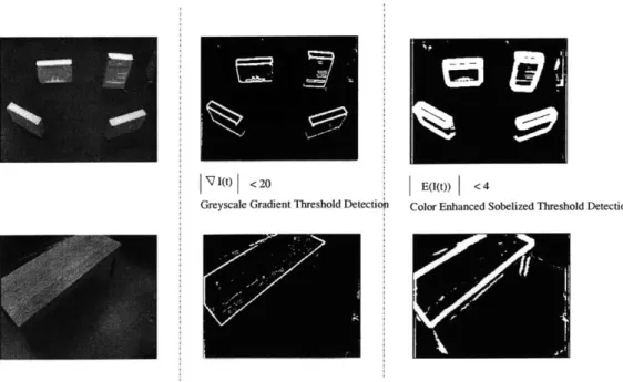
The choice of E(-) will, in general, trade off robustness to environment variability and speed of computation. The detection algorithm used on Erik requires significantly more computation than the gradient threshold edge detection employed by Horswill for processing Polly's greyscale image stream. Specifically, the edge detection process works by first separating the image into RED, GREEN, and BLUE color plane images (r, g, b). A histogram profile is calculated for each, and the maximum intensity for each histogram is found as well as the maximum over all color planes. We then apply smoothing to each image before convolving with a Sobel edge detection filter, a standard edge detection filter often used in robot vision because of its high tolerance to variability in illumination conditions. The seperate edge strength images are then averaged together. However, we set to zero the edge strength of any pixel that comes from the edge image of maximum color plane intensity, for which the intensity value is reasonably close to the maximum value. This reduces the detector's dependence on uniform lighting by helping to eliminate edges which come from the reflectance of overhead lights on the floor even in the presence of slowly changing floor color perception. The resulting averaged edge strength image is then thresholded to give a binary edge detected image. Compared with thresholding the image resulting from applying a first-order gradient differencing operator, the visual processing described here requires approximately O(n) pixels more computation. The detector used has been found to be much more robust to changes in room lighting and to shadow-casting objects which violate the GPC, like tables and chairs. In Figure 2.3, which shows the comparison between the two detectors for a set of styrofoam blocks and for a wood grained table, the color enhanced detector used by Erik picks up the table legs and the table shadows and chairs in the background, but also incorporates shadows cast by the styrofoam blocks. So the tradeoff in extra computation for more robust detection in the face of constraint violations is somewhat offset by the perception of somewhat fuzzier or enlarged obstacles. This is not necessarily a bad thing when
(t) < 20
Greyscale Gradient Threshold Detectiop
E(I(t)) <4
Color Enhanced Sobelized Threshold Detection
Figure 2-3: Comparison of Edge Detectors : detector used by Erik picks up the legs of the table but also more shadows.
considering the problem of obstacle avoidance, and can even be viewed as providing an additional boundary cushion or error margin.
2.2.2
Using the Obstacle Detector for Reactive Control
For a holonomic robot with a relatively low center of gravity, a simple reactive obstacle avoidance control system can readily be constructed from RDMt (u) whose qualitative behavior is invariant with respect to any strictly increasing function
f(-)
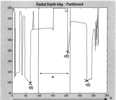
applied to RDMt(u). This is important for a reactive controller because it obviates the need to find the transformation mapping pixel distance to true metric distance as a function of radial direction. Horswill's collision avoidance routine, described here for completeness, bears similar relation to the scheme employed by the Actuator Control module for both head and base actuation. The controller partitions RDMt(u) intoFigure 2-4: Partitions of the Radial Depth Map : 1(t), r(t), c(t) marked.
three freespace functions, left, right, and center:
1(t) = minn<nRDMt(u)
r(t) = minu>uRDMt(u) (2.4)
c(t) = mini1.,_,<mRDMt(u)
where u, is the u coordinate of the center column of the image, and w is an implementation-dependent width paramter. Figure 2.4 shows the values for the radial depth map from a single image and pose of the styrofoam blocks (w is taken to be approximately twenty percent of the field of view). Although translation and rotation are coupled for a holonomic base, treating them as approximately separable allows us to model each degree of freedom by a first-order, zero delay subsystem. This allows for simple proportional control of the form:
0(t) = co(l(t) - r (t)) (2.5)
where 0(t) is the rotational velocity of the robot, v(t) is its translational velocity,
dmin is the closest the robot should ever come to an obstacle, and co, c, are user
defined controller gains. This controller will cause the robot to turn in the direction of greater freespace at a rate proportional to the difference in freespace in the left and right hemispheres of its field of view; and drive forward or backward proportional to its distance from the nearest obstacle in view. This is a reasonable choice for reactive control. When the robot is in open space the robot can move quickly and turns only a little in each control cycle. In more cluttered spaces, the projection of obstacles in the image has more drastic influences, and the robot will turn more and slow down to avoid impending collision. If the robot can actively tilt its head, the robot can keep the nearest object in its field of view at near constant height in the image by applying the head tilt control law:
0(t) - co(c(t) - do) (2.6)
where 0(t) is the head tilt velocity, and do is the desired distance to the nearest obstacle and should be greater than dmin. This will stabilize c(t) about the desired operating point causing the robot to continuously drive forward at near constant velocity, except when the limits of head tilt are reached. Unfortunately, at the time of writing, the pan-tilt unit had trouble smoothly actuating, so the camera head had to be locked in a static downward tilt for the system tests results discussed in this thesis. The negative impact this had on overall system functionality is discussed in chapter 7.
2.3
Subsystem Analysis
Horswill's algorithm preforms well under a variety of real indoor environments where noise caused by carpet stains, specular reflection off metallic surfaces, irregular or non-uniform lighting resulting in strong shadows, violate the algorithm's idealizations. The algorithm's failure modes under these less-than-perfect conditions usually results
in safe behavior since the robot's image operators prefer false-positives (the floor is really clear, but something is detected) to false-negatives (the floor is obstructed, but nothing is detected).
Horswill's algorithm is a purely reactive control mechanism: it forgets about ob-stacles once they are out of view. Combined with other perceptual processes and reactive controllers in a subsumption architecture [2] a robot agent can be directed to traverse hallway corridors and open atriums all the while relying on the obstacle avoidance routine to steer it toward freespace. However, navigation requires more than just reacting to what can be directly sensed: it requires some memory of recent experience, and a good sense of how to efficiently use this knowledge to achieve its goal oriented task.
Chapter 3
Depth Recovery
In order to aggregate visual information over time, the robot transforms a radial depth map RDMt(u) into approximate metric depth information. It will then integrate this transformed data into its temporary occupancy grid, the discrete 2-D map in floor coordinates that represents the robot's current beliefs about where obstacles are in the world. The inverse of the perspective projection transform found from doing a linear constrained optimization with known calibration points proved to be accurate enough for this purpose.
3.1
Perspective Projection Camera Model
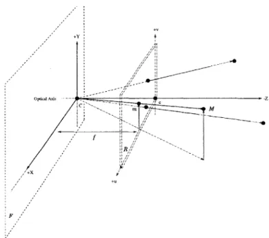
Figure 3.1 illustrates the perspective projection camera model. In this model per-spective rays or lines between points in the real world M(x, y, z) and a point of convergence known as the center of projection (COP) intersect the image or retinal plane R at points m(u, v). The perspective ray running perpendicular to R, and passing through c is called the optical axis, and the COP sits at a distance f, a focal length away. We are free to choose the origin C of our world coordinate system to be fixed at the COP with the z-axis pointing along the optical axis. This configuration is called the standard coordinate system of the camera, and defines the focal plane F to be the xy-plane. The perspective transform will allow us to describe the relationship between points in the image and points in any world coordinate system more easily.
+ 4
Optical Axis
fI
F
Figure 3-1: Perspective Projection Camera Model
3.1.1
Perspective Transform : Affine Equations
Following closely the derivation of the perpective projection transform described in [4], we see from our camera model that that the relationship between image coordinates and 3-d space coordinates via similar triangles can be written as:
U V
-f
x y z
(noting c sits at -f along the z - axis). The affine equations which then describe a point in the image are given by
-f U = -x z -f V = y; z
however, if the axes of the retinal plane have different scalings due to the geometry of the lens or imaging array elements, and the retinal plane origin is not aligned with
c, then these equations become U = + UO (3.1) z - f kv -= y + vo, (3.2)
where (uo, vo) are the image coordinate offsets of c, and ku, k, are the proper scalings of the retinal plane axes. Letting au = -fku and a, = -fk,, we can write this
equation linearly as U au 0 UO 0 V = 0 a, VO 0 (3.3) S 0 0 1 0 where ur =U/S v=V/S ifS O. (3.4)
According to the equation, as z approaches zero, the 3-d point M will be in the focal plane of the camera, and u and v will approach infinity. The set of points for which S = 0 are called the points at infinity and illustrate that the equation is
projective, i.e., defined up to a scale factor
[4].
If we allow for a different choice of world coordinate system, we can describe M',
our 3-d point M expressed in terms of the standard coordinate system, by the equation
M' = RRM + t, (3.5)
where Rj is a rotation matrix about the 3-d coordinate vector x' and t is the world coordinate system origin's translation vector offset in the standard coordinate system's frame.
3.1.2
Projective Geometry
Projective coordinates allow us to embed this affine transformation in our imaging equation using a linear algebra operation, by defining our world coordinates relative to a scale factor T. Using the projective coordinate (X, Y, Z, T) of M(x, y, z) we can rewrite the imaging equation as:
U V = S
-v-
-[
a 0 0 0 av 0 UO VO 1 0 0 0-I
X Y z T (3.6)which we write in matrix form as
f~n =
5=1
(3.7)The tilde notation is used here to denote a matrix or vector that lies in a projective space. Note this differs from equation 3.3 in that both image and world coordinates are defined up to a scale factor. We can always recover the true world coordinate
by dividing through by T, in other words, M(x, y, z) = M(X/T, Y/T, Z/T). Our coordinate transformation in equation 3.5 is invariant with respect to scale factor T,
so we can write it as:
MI' = R + t (3.8)
where
Rxyz 03
and
-t
0
We can concatenate these expressions into a single 4x4 matrix
~Rxyz t
K=-03 1
and the imaging equation for arbirtrary choice of retinal and world coordinate systems can then be written more simply as
~hn=M (3.9)
where P SK. Faugeras[4] gives a geometric interpretation of the row vectors of the
matrix P; they define the focal plane and the line joining the optical center to the origin of the coordinates in the retinal plane.
3.2
Camera Calibration
The process of camera calibration is the estimation of the matrix
P
from a set of known 2-d image and 3-d world point correspondences. If we think of the 3x4 matrix P as[
P p the concatenation of a 3x3 matrix P and a 3x1 vector T we again see the imaging equation as the affine transformU X
V =P y + (3.10)
S z
For N calibration points, let ni be the set of homogeneous image reference points, and Mi their corresponding 3-d world points. The projection matrix can be found
Reprojection of Calibration Points
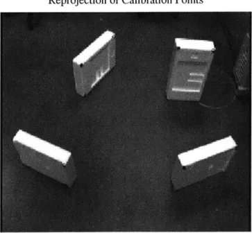
Figure 3-2: Calibration Pattern : Black tape reference points, and red circles show their calculated reprojection.
by minimizing a least-squares cost function of the form
E = ||i~n - (PM + )2(3.11)
with respect to P and P'. By writing the relationship between the affine coordinates of the reference points Mi and mi linearly, and adding the constraint that the plane of points at infinity has unit energy to avoid the trivial zero solution, this equation can be solved as a constrained linear least squares problem.
Let pi be the ith row of matrix P, and ]j5 be the ith element of row vector P; then affine equation 3.10 can be rewritten as:
PI- uip3M + Pi - UiP3 0
pM- vp Mi + P2 - =
This defines a system of 2N homogeneous linear equations in the unknowns of the elements of the projection matrix for our N calibration point pairs. In matrix notation we write
AP = 0
where A is a 2N x 12 matrix depending on the 3-D and 2-D calibration point pairs,
and p is the 12 x 1 vector [PT, 1i, P2, P2, P , P3]. Since f is defined up to a scale
factor, we avoid the trivial solution
P
= 0, by finding a solution as the minimizationof ||Aq| subject the constraint that
ItP3
12 1.Glossing over some details, we have 2N equations for each point pair correspon-dence, and 12 unknowns, therefore for N > 6 points a solution to our equation exists. In practice, the camera should be calibrated about its operating position, i.e. tilted down at some fixed angle, and more many more points than needed, widely scattered to cover the complete viewing area should be used to improve the accuracy of the results. In addition, these points should be sampled at various heights from the floor plane to avoid ill-conditioned or badly scaled matrix inversions in finding a solution. Table 3.1 shows the calibration point correspondences, the found projection matrix, and error statistics for the calibration pattern shown for a fixed camera tilt position of qf -0.8rad downward from horizontal at a height of 1.245m. Figure 3.2 shows the calibration pattern, and reprojection of the 3-D reference points. A Matlab code implemention of this calibration technique is included in Appendix A, and an in depth look at the process of constrained minimization and the conditions under which it will succeed for the equations described here can be found in [4].
3.3
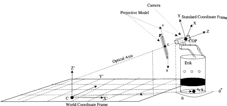
Recovering Floor Coordinates
The robot's camera is mounted facing forward on a "Directed Perception" pan-tilt unit which sits atop the robot's body only a few centimeters behind its front face. With the camera at a fixed tilt, the estimated projection matrix P accounts for any
Table 3.1: Calibration Data and Estimation Statistics x y z u v -0.6000 1.0050 0 31.4677 166.1140 -0.3000 0.9000 0 88.2419 190.6754 -0.3000 0.9000 0.2000 81.6060 168.2193 -0.3000 1.5000 0 107.4124 91.7281 -0.3000 1.5000 0.2500 102.2512 58.7456 -0.1000 1.8000 0.2500 145.7535 27.1667 0.3000 1.5000 0.3800 226.1221 40.5000 0.5350 1.5000 0.3800 271.8364 44.0088 0.3000 0.9000 0.2000 234.2327 169.6228 0.6000 1.0050 0.2000 301.3295 147.8684 0.3000 0.9000 0 225.3848 194.8860 Projection matrix: 276.5031 P - 9.8268 0.0199 108.6529 -136.7732 0.6519 -109.2647 -263.1310 -0.7580 94.1431 356.7305 0.6346
I
Intrinsic Camera Parameters:
[
a, = 273.6204 a, = 275.3820 uo = 159.1541 vo = 110.4814]
Extrinsic Parameters: 0.9990 0.0277 0.0199 0.0179 -0.7582 0.6519 0.0416 -0.6514 -0.7580I,
-0.0250 1.0408 0.6346I
Pixel Error Statistics :ISE = ncalculated -T e -112 16.6652 M-mreference -= 1.4978 1.4978
1
16.2601 MaxError(u, v) = [1.3910,2.1572], MinError(u, v) = [-2.2050, -2.1157]Camera
Projective Model
r Standard Coordinate Frane X Ernk V ZZ U 00 0 Y1 C
x0
World Coordinate Frame
Figure 3-3: Recovery of Floor Coordinates: World coordinate system rigidly attached to the floor.
deviation of the camera's mounting from perfect on-center alignment. The goal here is to recover the 3-d world coordinates of points in the image given that the imaged point came from a point on the floor. According to the projective transformation above, we can find our world coordinates based on the homogeneous image coordinates from the following recovery equation:
X U
y[ = P-
[
- P 1 p. (3.12)Z S
However, the robot only knows the affine image coordinates (u, v), and must deter-mine the homogeneous scale factor S. Using a 3-D world coordinate system fixed to the ground plane with z-axis normal and pointing up as in Figure 3.3, the scale factor
Recovery of Image Points from World Coordinates
Figure 3-4: Accuracy of Floor Coordinate Recovery
ijth component, and Pi be the ith component of
f,
then for z = 0 we haveW31(U - ) + W32(V - P2) + w 33(S - P3) = 0, (3.13)
which upon substitution for U = uS and V = vS and some rearranging of terms gives
the solution
S = W31P1 + W32P2 + W33P3 (3.14)
w31u + W32v + w33
from which the floor coordinates x and y can be found from backsubstitution of
S into the recovery equation. However, recovery of the floor coordinates changes
with translation and rotation of the robot. A standard change of coordinates is performed to map floor coordinates (x, y) obtained from the recovery equation, into true global floor coordinates (x', y'), based on the robot's estimated heading 0 and
position (xr, yr):
x' cos(O) sin(6) x x
y
[
- sin() cos(9)1 [y:
In the current implementation, this odometric information is taken from shaft en-coders in the robot's base, but could be made more robust if estimated from optical
flow, or by map based realignment. Figure 3.4 illustrates the reprojection of the floor
coordinates calculated from a radial depth of the styrofoam block calibration image. From this picture we see the accuaracy of our calibration, i.e., where the robot thinks these objects are in the world.
Chapter 4
Occupancy Grid Map
4.1
Constructing Occupancy Grids
Robust navigation requires planning, and planning requires having a map. With the ability to recover the real world coordinates of image pixels lying on the floor, the robot builds a map of the floor space for its surrounding environment. The mapping technique employed was derived from the occupancy grid method pioneered
by Moravec and Elfes [8]. An occupancy grid is a finite element 2-D grid which models the accumulation over time and space of information collected from a sensor or group of sensors. This technique, which has been employed by numerous robot researchers, discretizes the floor space of the room into uniform blocks, or grid cells, and assigns to each a value between 0.0 and 1.0 measuring the degree to which the robot believes there is an obstacle somewhere in that cell. While occupancy grids are easy to build and maintain, the accuracy of the robot's sensing information decays over long distances, and so we intend to use the occupancy grid fairly locally, for crossing a room, for example then throw them away. The robot will build more abstract, topological maps for large-scale navigation.
4.1.1
Background on Use and Application to Vision
While the occupancy grid mapping technique has been used extensively for sonar sensing robots, its employment for vision based robots has not had as wide appeal. One reason for this maybe the added complexity of transforming image pixel data into metric depth information, or because until recently cheap on-board off-the-shelf hardware capable of processing such information in real time has not been available.
A more likely reason is the awkwardness of using vision to construct occupancy grids.
Sonar sensing robots generally get information about a bounded 360 degree view around the robot at each time instance, while a robot with a forward looking camera must look around to acquire similar information. Some researchers have even gone to the extent of using a ceiling facing camera with an ultra-wide field of view and then accounting for image warp in software, as a means of dealing with the irregularity of the robot's sense-space geometry. Regardless of the reason for its lack of widespread appeal, vision based grid maps can be as robust as their sonar equivalent.
The nature of vision data also differs significantly from sonar data. In vision, the resolution of a single pixel and the overall field of view is dependent only on the camera's focal length. Sonar data is generally sparse: the field of view sampled from a single sonar is approximately a 30' conic wedge. Vision is also a passive sensor, recovering depth information indirectly. Sensor noise in vision, apart from that resulting from the camera's pixel acquisition electronics, is dependent on the degree to which the depth recovery model's assumptions match the given environment. The algorithm used in this paper prefers false-positives to false-negatives. On the other hand, sonar suffers from the problem of "missing objects", because reflections off corners known as specular reflection and wave absorbtion by roughly textured surfaces makes obstacles seem far away or absent. Since this sensor noise is usually modelled as an additive gaussian process with variance as an increasing function of range, the average of several adjacent sonar sensor readings is usually used to reduce its chances of error over time. Erik is typical of most grid mapping research robots, having 24 sonars arranged in a ring around its midsection. Although the height of the robot's
sonar ring dictates the maximum sensing distance as the boundary where the sonar's conic wedge intersects the floor, its effective sensing distance may be considerably smaller given the sensitivity of the sonar's receiver electronics.
4.1.2
Integrating Occupancy Evidence
In this thesis work, we applied a Bayesian update rule for the integration of newly acquired freespace/obstacle information into the occupancy grid. The update rule we used is like the one employed by Thrun at CMU [11] for use on sonar sensing robots, but is modified for use with visual sensing.
The update proceeds as follows. Each radial depth map (RDM) that the robot gets gives information about occupied and free areas in its field of view. We recover floor coordinates for pixels in the image which generated the RDM under the assumption that all pixels were imaged from the floor, and map them into grid cells. Now we have to combine the newly sensed evidence with our previous beliefs about the state of the world. We make the assertion that data is "new" if and only if the robot's pose has changed significantly. This helps simplify the update rule by allowing us to assert a greater degree of conditional independence between sensor samples given the state of the world. Formally speaking, we only perform an update if
AS > ASthresh
where As = st - st- is the change in robot pose since the previous update, ASthreh
is some user defined threshold, and st = (x, Y, Obase, Ohead, &head) is the robot's pose at
time t. Next we define
X
(U, V) : (U, V) F- (X, y)as the mapping from image pixel (u, v) to the grid cell containing floor coordinate
(x, y) under the supposition that every pixel lies on the ground; then we can find the
-Erik 0 00 ---- - --- --- --- 1...0 Unoccupied Cells Occupied Cells Unknown
Figure 4-1: RDM gives grid cell occupancy information.
to construct observations for each grid cell (x, y) given the robot's pose, which we describe mathematically via the function
r
occupied 0(x,y) (St) unoccupiedunknown
if Eu s.t. X(u, RDMt(u)) = (x, y), if $ v > RDMt(u) s.t. X(u, v) = (x, y),
otherwise.
This functions says that we should declare a grid cell: occupied if there exist any pixels in the RDM which map into it, unoccupied if and only if all pixels that map into it come from pixels below the height of the RDM, and unknown if pixels mapping into it are above the RDM or otherwise. Figure 4.1 illustrates for us the observation of an RDM.
It is convenient to interpret the output of this observation function as sampling a random process where each sample yields an i.i.d random variable having
Pr(OCC(x,y) | 0() Z.
Y'
C
World Coordinate Frame
(the notation Oik) denotes the kth observation for grid cell (Xly)
(x,
y)). This probabilityof occupancy given the kth observation is extremely difficult to model. Although such models may be learned by training neural networks, we have chosen to design our model by hand. Lacking a proper probability distribution of conditional occupancy given observation, a simpler approach was taken in this thesis, whereby the user chooses update rates a and / that satisfy the constraints
pr(OC("Y I 0 (k)
Pr(occ(2,)
|
(X = occupied) < a 1.0 - Pr(occ(,y) I 04xy> = unoccupied) > 3.The parameters a and 3 allow us to assign a degree of trust to our observations. We'll assign larger values of a and
#
if we have reason to believe that our sensor can be trusted, and lower values in noisier environments where our obstacle detector is more likely to make mistakes. This simple modelling allows us to approximate a measure of the true probability of occupancy for grid cell (x, y), as the probability of occupancy for grid cell (x, y) conditioned on all observations,Pr(occ(,) 1 0(), t ,(2) ... , O( ).
If we assume that each "process sample" is taken at significantly different robot
pose, we can assume a modest degree of conditional independence, in other words, Pr(occ(,y)
I
O ) Pr(occ(x,y) O(")), if k :4 k', even though the statistics( k)Y (k')
of observation Pr(Ok) ) and Pr(O(k)) are usually dependent. This assumption is difficult to justify. In fact, we argue that it is probably not true and will depend on the correlation decay time of our measurements. The difficulty in determining a good sensor model hinges on the fact that this is a complicated function of the robot's velocity and varies spatially in the image plane for different tilt angles, and lighting conditions. The remaining derivation of the Bayesian update process treats our pseudo-sensor model as though it were legitimate according to the assumption of conditional independence.
Bayesian Updating
Given a sensor model whose output for update k is
pr(occ(",Y) I ON'k)
we can estimate the probability of occupancy given N observations iteratively by successive application of Bayes' rule and the assumption of conditional independence. Without detailing the derivation, the resulting update is captured by the formula
Pr(occ(X,Y) O() (,)y,) ... , ((N)
Pr(OCC(x,y) 1 0') N Pr(ocC(XY) O()
Pr(occ(,J) 1 0' )k2 - Pr(occ(X,Y) I O )
1 - Pr(OCC(x,y))
Pr(Occ(XY))
(4.2)
where Pr(occ(,y)) is the prior probability for occupancy, sometimes referred to as the background occupancy, and is representative of the average occupancy of a grid cell in a mature map [11]. In our experiments, we found that good occupancy grids are constructed when the background occupancy is approximately 0.35 for hallways, but should be higher in more cluttered environments like the lab room where Erik resides.
Modifications to the Rule
The following change to the occupancy probability update equation was applied, to
accomodate for the lack of a direct sensor model:
Pr( occ(x,y) 1 0() 0(2) O(N))
(, (x)' ' (x,y)
1 Nc Pr(occ(xy) ) -1...,
S-1 + N 2P c() (x)(t) = occupied,
1 - + Hk2 1_Pr(occ(, 1 Pr(occ( ,y), I O k Pr(ocC( ,)) / i ()Pr(occ(,()) )(t) = unoccupied,
1 -1+ )I fN k=2I-r~cq~y y (k) xy) Ixy() -1rocx,) fOXl)t = u ncuidk o R
(i _ Pr(occ(x,,y) I O~k 1-Pr(occq,,y))
k=
+ 1-Pr(occ(x,y) 10 (k) Pr OCC (X,) Y) if 0(,Y) (t) -unknown.
(4.3)
Since the occupancy grid probability represents all previous applications of the up-date rule, the previous value can be substituted for the probability of occupancy conditioned on all previous observations. In the case where O(,y) (t) = unknown, the occupancy probability is unchanged. Figure 4.2 gives an example of the evolution of the occupancy grid as the robot drives around the lab room. The images on the left show a snapshot of what the robot sees (the pink shading indicates pixels above the RDM). The images on the right depict the occupancy grid map. The blue square marks the robot's position at the labelled control step, white areas indicate freespace, black areas are obstacles, and grey areas have not yet been explored. Between control steps t = 4 and t = 90, not shown in the sequence, the robot has driven around the
room and discovered the back wall. Control steps t = 90 and t = 91 shows the robot
viewing the same styrofoam blocks from an alternate viewing angle. We can clearly distinguish the layout of these blocks on the floor; they are the dark obstacles at near the bottom of the explored space in the map at step t = 91.
0
CNl
C,,
NC,.
Chapter 5
Navigation: The Planning Module
5.1
The Agent-Environment Feedback Model
Environment
State
Action
0 0 0 0
Figure 5-1: The Agent-Environment Feedback Model
Consider the problem of robot navigation as represented by an agent in an envi-ronment for which a state-space description can be written. The state-space evolves according to a Markov process, and the action of the agent is described as a function of the current state at every point in time. For the system described in this thesis,
the occupancy grid captures the robot's belief about the underlying structure of this process. As the robot drives around it continuously gains information which it aggre-gates into its occupancy grid. In the limit of a large number of observations, grid cell occupancies approach their final or mature values with probability 1. Therefore, any description of the state of the world that has a counter-factual belief for a grid cell's occupancy in the interim, must have a transition probablity of 0. For example, the state of the world would be contradicted if the robot occupied a group of grid cells that it earlier claimed were occupied by something else. The universe of belief states about the world is therefore constantly shrinking as more grid cell's occupancy be-comes known with certainty; the Markov process is converging to a steady-state and is in fact converging to a single unique state of the world we call the full-information state. Explicitly speaking, as it drives around integrating information collected at dif-ferent poses, the occupancy grid becomes increasingly refined according to a Bayesian updating process, and the robot's belief about the global structure becomes known with certainty.
The robot's behavior is affected by its current state of knowledge about the world. Conversely, the rate of flow and content of information about the world are affected
by the robot's action choices in each period. For example, the appearance of a box
in a narrow hallway may mean that the most direct path is blocked and that the robot should look for an alternate route to its goal or desired destination, possibly through another room or hallway corridor it has not yet seen. Clearly, its actions (actuator velocities) alter its pose, possibly exposing previously unseen details of the world which may cause it to react differently in the future. In addition, the robot
may pay a penalty for not finding an alternative route quickly enough. Perhaps it is in need of a recharge and every second it spends looking for a way around the hallway obstacle, the longer it will have to spend at the charging dock. The robot's navigation strategy should therefore try to seek out the best possible alternative as the route that allows the robot to get to the goal in the shortest amount of time. Navigating efficiently in this sense is then tantamount to finding a trajectory through the state-space that minimizes the cumulative cost for getting to the goal. Since the
robot's future is largly dependent on its current actions, position, and knowledge of the global space, we look to the theory of Markov decision processes (MDP)s and optimal control for finding good navigation strategies.
5.1.1
Overview of Markov Decision Processes
An MDP models the synchronous interaction that takes place between a goal seeking agent and its environment as it tries to minimize some cumulative cost function. In general it is defined by a set of states, action, the one-step dynamics of the environ-ment, and a penalty signal. Formally we define this penalty signal which passes from the environment to the agent as a sequence of numbers, ct
C
R. Since the agent's goal is to minimize the total amount of penalties it receives while interacting with the environment, we define the cumulative cost Ct as the sum of penalties paid at each future time step:Ct ct+1+ ct+2 + ct+3 + + cT
where T is a final time step, or the end of an episode (finite-horizon). We can also define the discounted cost for continuing or non-episodic tasks T = oo (infinite-horizon), as:
00
Ct = ct+1 + 'yct+2 + 'Y2 ct+3 + Z yk ct+k+l
k=O
where the discount factor y E [0, 1] measures the degree to which future costs will impact current decisions.
We represent a finite-state MDP by the tuple, (S, A, T, C) where:
" S the finite set of states in the world.
" A the finite set of actions for every state.
" T : S x A x S -+ [0,1] is the set of transition probabilities, and T(s, a, s')
Pr(st+1 = s' I st = s, at = a), defines the transition probability function, which quantifies the one-step dynamics of the state-space as the probability of going to state s' from state s by taking action a.
* C : S x A -+ C defines the costs for being in each state s, and acting according to some behavior policy.
C(s, a) = E [ct+i
I
st = s, at = a, st+1 = s'1represents the immediate or expected value of the next penalty paid for transi-tioning to s' taking action a in state s.
In general, the expected cumulative cost will be dependent on the trajectory that the agent follows over the course of an episode or lifetime in the infinite-horizon case. The agent's trajectory is the direct consequence of its actions, which are selected by the agent in each state according to some control or policy 7r(s, a): a mapping from
situations (states) to actions defined with respect to a value function - a function of state (or of state-action pairs) that estimates how good it is for an agent to be in a particular state (or to perform a particular action in a given state) [10]. The policy function 7r*, characterizes optimal behavior for the agent, and is the unique mapping of situations (states) to actions that minimizes the expected discounted future cost
E E itct