HAL Id: hal-00280305
https://hal.archives-ouvertes.fr/hal-00280305
Submitted on 19 Feb 2021
HAL is a multi-disciplinary open access
archive for the deposit and dissemination of
sci-entific research documents, whether they are
pub-lished or not. The documents may come from
teaching and research institutions in France or
abroad, or from public or private research centers.
L’archive ouverte pluridisciplinaire HAL, est
destinée au dépôt et à la diffusion de documents
scientifiques de niveau recherche, publiés ou non,
émanant des établissements d’enseignement et de
recherche français ou étrangers, des laboratoires
publics ou privés.
Analysis of ground-measured and
passive-microwave-derived snow depth variations in
midwinter across the northern Great Plains
A.T.C. Chang, R.E.J. Kelly, E.G. Josberger, R.L. Armstrong, J.L. Foster,
N.M. Mognard
To cite this version:
A.T.C. Chang, R.E.J. Kelly, E.G. Josberger, R.L. Armstrong, J.L. Foster, et al.. Analysis of
ground-measured and passive-microwave-derived snow depth variations in midwinter across the northern Great
Plains. Journal of Hydrometeorology, American Meteorological Society, 2005, 6, pp.20-33.
�hal-00280305�
Analysis of Ground-Measured and Passive-Microwave-Derived Snow Depth Variations
in Midwinter across the Northern Great Plains
A. T. C. CHANG,* R. E. J. KELLY,⫹ E. G. JOSBERGER,# R. L. ARMSTRONG,@ J. L. FOSTER,*AND
N. M. MOGNARD&
* Hydrological Sciences Branch, Laboratory for Hydrospheric Processes, NASA Goddard Space Flight Center, Greenbelt, Maryland ⫹ Goddard Earth Sciences and Technology Center, University of Maryland, Baltimore County, Baltimore, Maryland
# U.S. Geological Survey, Tacoma, Washington
@ National Snow and Ice Data Center, University of Colorado, Boulder, Colorado & Centre d’Etudes Spatiales de la Biosphère, Toulouse, France
(Manuscript received 3 February 2004, in final form 26 August 2004)
ABSTRACT
Accurate estimation of snow mass is important for the characterization of the hydrological cycle at different space and time scales. For effective water resources management, accurate estimation of snow storage is needed. Conventionally, snow depth is measured at a point, and in order to monitor snow depth in a temporally and spatially comprehensive manner, optimum interpolation of the points is undertaken. Yet the spatial representation of point measurements at a basin or on a larger distance scale is uncertain. Spaceborne scanning sensors, which cover a wide swath and can provide rapid repeat global coverage, are ideally suited to augment the global snow information. Satellite-borne passive microwave sensors have been used to derive snow depth (SD) with some success. The uncertainties in point SD and areal SD of natural snowpacks need to be understood if comparisons are to be made between a point SD measurement and satellite SD. In this paper three issues are addressed relating satellite derivation of SD and ground mea-surements of SD in the northern Great Plains of the United States from 1988 to 1997. First, it is shown that in comparing samples of ground-measured point SD data with satellite-derived 25⫻ 25 km2pixels of SD
from the Defense Meteorological Satellite Program Special Sensor Microwave Imager, there are significant differences in yearly SD values even though the accumulated datasets showed similarities. Second, from variogram analysis, the spatial variability of SD from each dataset was comparable. Third, for a sampling grid cell domain of 1°⫻ 1° in the study terrain, 10 distributed snow depth measurements per cell are required to produce a sampling error of 5 cm or better. This study has important implications for validating SD derivations from satellite microwave observations.
1. Introduction
With the continued growth in world population and industrial and commercial productivity, demands on global water resources have increased greatly. For ef-fective water resources management there is a need to accurately quantify the various components of the hy-drological cycle at different space and time scales. Snow is a renewable water resource of vital importance in large portions of the world and is one of the major hydrological cycle components. It is also a major source of water storage and runoff for many parts of the world. For example, in the western United States snow con-tributes over 70% of total water resources. To better predict snow storage and detect trends in the variations of water resources, accurate snowpack information with known error characteristics is necessary.
Traditionally, rulers, fixed snow stakes, and snow boards are used to measure the snow depth (SD) at a point. In general, point measurements of SD produce high quality data representative of a small location (⬍10 m scale length). To monitor SD in a temporally and spatially comprehensive manner, optimum interpo-lation of the points must be undertaken (Brasnett 1999; Brown et al. 2003). However, the spatial representativ-ity of point measurements in a basin or at larger scale is uncertain (Atkinson and Kelly 1997). Furthermore, the spatial density of SD measurements in most parts of the world is rather low. Thus, the accuracy of spatially in-tegrated point measurements of SD needs to be as-sessed carefully.
Spaceborne scanning microwave sensors, which cover a wide swath and can provide rapid repeat global coverage, are ideally suited to augmenting global snow measurements. For example, passive microwave radi-ometers such as the Scanning Multifrequency Micro-wave Radiometer (SMMR) on Nimbus-7 and Seasat-A and the Defense Meteorological Satellite Program
Corresponding author address: Richard Kelly, NASA Goddard
Space Flight Center, Hydrological Sciences Branch, Code 974, Bldg. 33, Greenbelt, MD 20771.
E-mail: rkelly@glacier.gsfc.nasa.gov
(DMSP) Special Sensor Microwave Imager (SSM/I) have been utilized to retrieve global SD. To assess the representativity of satellite-derived SD, it is necessary to determine how and whether the point SD measure-ments can be compared with the spaceborne-derived SD that typically represents about 25⫻ 25 km2in area. The uncertainties in point and areal SD measure-ments of natural snowpacks need to be understood if comparisons are to be made between point SD mea-surements and satellite-derived SD. The statistical ability of the snow depth, as represented by the vari-ogram, has a direct effect on the accuracy of SD derived from satellite data. Consequently, it is essential that the magnitude and cause of any variability is clearly de-fined for robust global validation of satellite-derived SD. In this paper we use sparsely distributed SD data from the National Weather Service (NWS) cooperative station network and SSM/I-derived SD data to study large-scale snow distribution.
To understand the snow-distribution characteristics from ground-measured SD, it is necessary to know the density of point SD measurements and the defined SD areal accuracy. Geostatistical analysis can be used to gain a better understanding of the spatial variability of snow depth in large areas, such as the northern Great Plains. Although there are large portions of the world where the spatial density of point-measured SD is less then 1 per 10 000 km2(approximately about the area of
1° latitude by 1° longitude), the aims of this study are to understand and quantify statistically the uncertainties associated with sparse sampling of SD over a regional scale, and to determine how these uncertainties affect the validation of global SD derivations from satellite observations at a local to regional scale. The aim of this study is to find out how well remote sensing–derived SD can be validated by current ground-measured point SD data, specifically
1) How well does ground-measured SD compare with satellite-derived SD?
2) What are the characteristics of snow spatial distri-bution?
3) What are the sampling criteria for making ground snow measurements so they can be used to validate satellite-derived SD, given a predefined accuracy re-quirement?
Throughout the paper we refer to ground SD, which refers to the measurement of snow depth at a point made by a temporary ruler or permanent ruled staff. The snow depth is the accumulated vertical thickness of snow from the ground to the snow–air interface at any given moment.
2. Background
Any remote sensing technique that can estimate ac-curately snow storage is of great benefit for global
wa-ter cycle research and wawa-ter resources applications. With spaceborne satellite sensor data, global snow measurements can be achieved. Spaceborne sensors can image the earth with spatial resolutions varying from tens of meters (e.g., visible and infrared spectrom-eter; synthetic aperture radar) to tens of kilometers (e.g., passive microwave radiometers). Visible and in-frared sensor applications to snow are limited to clear-sky occurrences and are sensitive only to snow surface properties, while passive microwave sensors are solar illumination independent and are sensitive to snow vol-ume properties. Both remote sensing approaches have been used to monitor snow cover areas. With the im-provement in satellite instrumentation, regional and lo-cal slo-cales can now be mapped effectively. Passive mi-crowave sensors have been used to monitor continen-tal-scale snow cover area extent in the Northern Hemisphere for several years (Chang et al. 1987). How-ever, passive microwave retrieval methods of snow wa-ter equivalent (SWE) and/or SD are less mature than visible (VIS)/IR sensor mapping approaches and often result in large uncertainties from retrievals at the global scale (e.g., Armstrong and Brodzik 2001, 2002).
Microwave brightness temperature measured by spaceborne sensors originates from radiation from 1) the underlying surface, 2) the snowpack, and 3) the atmosphere. The atmospheric contribution is usually small at microwave frequencies and can be neglected over most snow-covered areas, especially at higher lati-tudes. In this paper, therefore, we neglect the atmo-spheric effects when extracting snowpack parameters from satellite data. Snow crystals within snowpacks are effective at scattering upwelling microwave radiation, and the microwave signature of a snowpack depends on both the number of scatterers and their scattering effi-ciency. The degree of scattering is frequency depen-dent, with higher frequency (shorter wavelength) radia-tion scattered more than lower frequency (longer wave-length) radiation. The deeper the snowpack, the more snow crystals there are available to scatter microwave energy away from the sensor. Hence, microwave bright-ness temperatures are generally lower for deep snow-packs, with a larger number of scatterers, than they are for shallow snowpacks, with fewer scatterers (Matzler 1987; Foster et al. 1997). The scattering effect increases rapidly with effective snowpack grain size; for example, when a depth hoar layer is present. Such large snow crystals often develop in thin snowpacks that are sub-ject to cold air temperatures at the snow surface and a large thermal and vapor gradient through the pack. This can result in very strong signals from thin snow-packs, as observed by Josberger et al. (1996) in a com-parison of microwave observations and snowpack ob-servations from the upper Colorado River basin. Based on radiative transfer theory, Chang et al. (1987) suc-cessfully developed a method to derive SWE using SMMR observations. SSM/I data have been used rou-tinely to infer the SWE in prairie and boreal forest
regions of Canada (Goodison and Walker 1995; Goita et al. 2003). Derksen et al. (2002) found that the time series of SSM/I SWE remains within 10 to 20 mm of surface measurements in the Canadian prairie. Walker and Silis (2001) reported derived snow cover variations over the Mackenzie River basin. Their algorithm was tested using “ground truth” in situ data and shows that the inferred SWE estimates generally underestimate the measured SWE by between 10 to 30 mm. The deri-vation of an accurate algorithm is complicated by the snow crystal metamorphism that occurs through the winter. To model this effect, Josberger and Mognard (2002) and Mognard and Josberger (2002) developed an algorithm for the U.S. northern Great Plains that includes a proxy for crystal growth based on air tem-perature. Kelly et al. (2003) coupled a spatially and temporally varying empirical grain growth expression with a radiative transfer model to derive SD in the Northern Hemisphere. All of these results encourage us to study further the interaction of microwaves with snow parameters to derive a validated algorithm with known errors.
Ideally, it is recognized that SWE is closely related to the volume of snowpack stored in a basin. However, global SWE datasets are not available; rather SD is the quantity that is recorded at many weather station loca-tions. Snow depth is measured at a point, usually from a ruler or snow board. In the high latitudes the distri-butions of liquid precipitation (rain) and solid precipi-tation (snow) are very similar. Precipiprecipi-tation gauges also have been used to record accumulated snowfall, al-though such devices are often subject to large uncer-tainties (Yang et al. 1998, 1999, 2000). Precipitation gauges are also sparsely distributed around the globe with large regional variations in spatial density. For ex-ample, in Germany there may be three–five stations in a 25⫻ 25 km2area (Rudolf et al. 1994). In the United
States there are some areas with one station in 25⫻ 25 km2while in some areas of Russia, for example, there is
typically only one station in area 100⫻ 100 km2. Snow courses provide more detailed measurements of snow parameters located at discrete sites along a defined transect; however, they are even sparser in occurrence. Thus, with ground SD data more readily available for comparison with satellite derivations, ground SD mea-surements are the prime validation source used in this study. Also, since SD is the most widely measured vari-able, we use the SD form of the microwave retrieval algorithm from Chang et al. (1987) in this study.
3. Snow field descriptions and data used in the study
The northern Great Plains study region covers a geo-graphical area from 42° to 49°N and 91° to 104°W. The test area is about 800 000 km2. This encompasses the
states of North Dakota, South Dakota, and Minnesota.
The geomorphology of this area is rather homoge-neous. For example, the Roseau River in Minnesota and Manitoba, Canada, is a typically small basin that flows into the Red River. The Roseau basin has rela-tively low relief (⬍500 m) with a mixture of cropland and forests (hardwoods and conifers). Recently Jos-berger et al. (1998) reported a comparison of the sat-ellite and aircraft remote sensing snow water equivalent estimates in this region. They found that in this prairie ecosystem passive microwave observations could be used to derive SWE. This area, therefore, is ideal for studying the characteristics of ground SD measure-ments and microwave-derived snow depths.
Snow depth retrievals were performed using obser-vations from SSM/I instruments aboard DMSP F-8,
F-11, and F-13 platforms. Ground snow depth
measure-ments, archived by the NWS and obtained from the cooperative network of observers, were collected for the study region. These ground measurements consist of daily weather observations of temperature, precipi-tation, snowfall, and snowpack thickness at more than 351 stations in the area, although this number varies from year to year. Typically, the snow depth informa-tion is collected daily but with a long time lag before the data become available. Cooperative station data for 12 February each year from 1988 to 1997 were used in the analysis. Figure 1 shows the location of the ground SD data within the northern Great Plains (NGP) study re-gion. All data were georeferenced to the equal area scaleable earth grid (EASE-grid). The SSM/I data were obtained from the National Snow and Ice Data Center (NSIDC) in 25⫻ 25 km2EASE-grid projection (Arm-strong and Brodzik 1995). For the SSM/I, with the ex-ception of 1994, our analysis focused on the mean of 3 days (10–12 February) for each year of 10 yr (from 1988 to 1997). This averaging process ensured complete cov-erage of the study region for the selected date. In 1994, because of incomplete SSM/I coverage, the 3-day mean was shifted to 27–29 January. Only morning SSM/I passes were used in the analysis (approximately 0400– 0600 local time).
The NWS cooperative station data can take some time to become available. This time frame represents a 10-yr period when paired observations of SSM/I data (launched in 1987) and NWS cooperative station data were available. These 3 days were chosen since they represent a time in winter when the snowpack is poten-tially at its most stable and extensive, with minimal liquid water content. Figure 2 shows five time series plots of mean daily minimum air temperature and mean daily snow depth from 1 January to 28 February at the five selected cooperative stations identified in Fig. 1. The data demonstrate that not only were the mean daily minimum temperatures well below 0°C, at this time of year the standard deviation of snow depth was generally small, as shown by the error bars in the snow depth time series. By undertaking the analysis for the same time in consecutive years, potentially consistent
biases in the data (either satellite or ground) could be identified. It was also decided that the analysis would focus only on midwinter snow packs. It is recognized that SSM/I-derived SDs in the early season underesti-mate field-measured conditions because snow is often highly discontinuous in space and time (Armstrong and Brodzik 2001). Also, in late winter and early spring, the presence of melt–refreezing events and snow that con-tains free liquid water is known to be a very challenging environment for SD estimates from passive microwave instruments (Stiles and Ulaby 1980). To investigate in-stances when confidence was high that only relatively stable and dry snowpacks were present, therefore, this research is concerned with SD estimates derived from passive microwave instruments during midwinter con-ditions only (January and February).
4. Data analysis
a. Comparisons of paired ground snow depth measurements and passive microwave snow depth estimates
Statistical analysis of paired ground SD and SSM/I SD for each year (from 1988 through 1997) and the 10-yr composite show that the SSM/I estimates gener-ally compare well with the ground SD measurements. Table 1 gives summary statistics for each year plus com-posite means. The mean ground SD is highly variable from year to year (1.5 to 45.4 cm). In the 10-yr period, there are 3 yr when SD is less than 10 cm, 5 yr when SD
is between 10 and 30 cm, and 2 yr when SD is greater than 30 cm. The corresponding range of SSM/I-derived mean SD (1.7 to 43.4 cm) is similar to the ground SD measurements, with the total composite mean SD from SSM/I estimates almost identical to that of the ground data. The correlation between yearly mean ground SD and SSM/I SD values for the period is 0.82.
The difference between ground SD and SSM/I-derived SD varies from year to year. The maximum difference of the means was 18.4 cm (1994). The mini-mum difference of the mean was found to be 0.1 cm in 1990. Generally there is a greater variation of snow depths observed for the ground data than the satellite-derived data. This is because the variability of snow at a point tends to be greater than that observed for a footprint that is a smoothed, integrated signal from within an instantaneous field of view. A statistical hy-pothesis test, the paired t test, was used to determine whether or not there were significant differences be-tween the ground and SSM/I-derived SD. The paired t statistic (t) is defined as
t⫽
共ⲐN1Ⲑ2兲, 共1兲
where and are the mean and standard deviation of the paired differences of the two variables (ground SD and SSM/I SD), and N is the number of data pairs (McClave and Dietrich 1979). For N⬎ 30, in this case
N⬎ 250, t follows approximately a normal distribution.
The hypothesis of difference is rejected if|t| ⬍ 1.96 at
FIG. 1. Shaded relief map showing the location of the snow depth measurement points within the northern Great Plains study region. The highlighted and numbered stations are sites used in Fig. 2.
Fig 1 live 4/C
the 95% confidence level. The paired t statistics are included in Table 1. Inspection of the t values shows no systemic pattern from year to year. There are 8 yr with |t| ⬎ 1.96 and 2 yr (1990 and 1997) with |t| ⬍ 1.96. For those years where the value of t is larger than 1.96, there is a significant difference between the ground SD and SSM/I-derived SD at 95% level confidence. The paired t-test value is –1.13 for the composite 10-yr dataset. The mean difference between the ground SD and satellite SD is 0.4 cm. However, the standard de-viation of the difference is 18.7 cm, which is slightly larger than both the accumulated ground and SSM/I snow depth means (17.9 and 18.3 cm, respectively). Overall, for half of the years the SSM/I-derived SDs are less than the ground SDs, and for the remaining 5 yr
they are more than the ground SDs. No significant ex-planation could be found to explain this feature for these bulk statistics. It is possible, however, that snow-pack stratigraphy variations at the local scale (and within the 25⫻ 25 km2SSM/I pixels) have an important
effect on microwave responses from the snow. While we assume in the retrieval algorithm that grain size and density are constant, spatial and temporal variations in snow stratigraphy can play a significant role in attenu-ating the upwelling radiation (Matzler 1987). Changes in the vertical properties of the snowpack are generally caused by thermal and vapor gradients through the snowpack along with the surface melt and refreezing of water (Colbeck 1982). Unfortunately, no information in the data is available on these properties for this
re-FIG. 2. Graphs of mean daily snow depth and mean daily minimum air temperature for Jan and Feb for 1988–97. The five selected sites are identified in Fig. 1. The error bars in the mean snow depth represent the standard deviation for the 2-month period.
search. It is probable, however, that variations in den-sity and grain size contributed to variations in SSM/I-derived SD in addition to variations in SD accumula-tion.
Measurement error is an important factor explaining why ground and satellite data have different statistical characteristics. Snow depth measured at a point reflects snow accumulation subject to local microscale pro-cesses, while SSM/I-derived SD reflects mean snow conditions, subject to controls at the local to regional scale. For example, wind speed is the most important environmental factor contributing to the undermea-surement of snow at a point (Goodison et al. 1989). In the NGP region, high wind speeds are common and cause a system bias error. At cooperative stations, typi-cally snow rulers or snow boards are used to measure SD. To obtain a representative SD measurement under snow drifting or snow scouring conditions, careful judg-ment by the observer is required. Assuming that such processes occurred with equal frequency over the study domain, a varying positive (drifting) or negative (scour-ing) bias from year to year might also help to explain why for half of the years the bias is positive and the other half negative.
b. An assessment of the spatial variation of
ground-measured and passive-microwave-derived snow depth
Large spatial and temporal variations exist in global and local snow cover extent and volume (Frei and Rob-inson 1999). Errors of these variations are not very well understood, although it is important for better climate observation. It is necessary to better understand the spatial characteristics of different scales of SD. Jacob-son (1999) defined five spatial-scale lengths of weather parameters: planetary scale (⬎10 000 km), synoptic scale (500 to 10 000 km), mesoscale or regional varia-tion (2 to 2000 km), microscale (2 mm to 2 km), and molecular scale (⬍2 mm). In the NGP study region, we are concerned with the characterization of snow distri-bution at the microscale and mesoscale.
From the t-test values of the previous section,
meso-scale (SSM/I) and micromeso-scale (ground) comparisons of snow depth revealed that for 8 out of the 10 yr, signifi-cant differences existed between these two datasets. However, when the data were aggregated over a longer time period (10 yr), the |t| value was less than 1.96, suggesting that when averaged over successive years the two datasets are not significantly different. To fur-ther understand these characteristics, analysis of the spatial variability of the two datasets was undertaken. The variogram, the central tool of geostatistics, can be used to examine the spatial dependency of a vari-able. It provides an unbiased description of the scale and pattern of spatial variation. Observations of a se-lected property are often modeled by a random vari-able, and the spatial set of random variables covering the region of interest is known as a random function (Isaaks and Srivastava 1989). A sample of a spatially varying property is commonly represented as a region-alized variable (e.g., as a realization of a random func-tion). The semivariance (␥) may be defined as half the expected squared difference between the random func-tions Z(x) and Z(x⫹ h) at a particular lag h. The semi-variogram (hereafter referred as semi-variogram), defined as a parameter of the random function model, is then the function that relates semivariance to lag:
␥共h兲⫽ 1Ⲑ2 E兵关Z共x兲⫺ Z共x⫹ h兲兴2其, 共2兲 where E is the ensemble mean of pairs. The sample va-riogram␥(h) can be estimated for p(h) pairs of obser-vation or realizations, [Z(xl⫹ h), l ⫽ 1, 2, . . . . p(h)], by ␥共h兲⫽ 1Ⲑ2p共h兲
兺
l⫽1 p共h兲 关Z共xl兲⫺ Z共xl⫹ h兲兴 2 . 共3兲A mathematical function or model is usually fitted to the experimental values, which are discrete, to repre-sent the true variogram of the region, which is continu-ous. The experimental values are often erratic because they are subject to error. In general, the variogram model is either unbounded (increases indefinitely with lag) or bounded (increases to a maximum value of semivariance, known as the sill, at a finite positive lag,
TABLE1. Ten years of mean () and standard deviation () of paired ground and SSM/I snow depth estimates and the paired
t-test values.
Year N Pairs Ground m (cm) Ground s (cm) SSM/I m (cm) SSM/I s (cm) Paired t value
1988 256 23.1 17.1 19.5 11.6 4.04 1989 265 16.3 19.0 14.3 11.6 2.24 1990 339 1.8 5.6 1.7 4.2 0.68 1991 351 1.5 4.1 4.4 11.3 ⫺5.57 1992 281 6.7 9.5 7.8 11.8 ⫺1.99 1993 269 19.5 11.0 29.4 15.5 ⫺9.54 1994 266 39.1 19.3 20.7 10.5 18.02 1995 271 10.3 12.2 22.7 19.5 ⫺12.15 1996 254 20.3 23.7 24.9 17.3 ⫺2.80 1997 275 45.4 29.9 43.4 13.8 0.96 1988–97 2762 17.9 21.9 18.3 17.9 ⫺1.13
known as the range a). The sill is equal to the a priori variance (that defined for an infinite region) of the random function (RF), while the range indicates the limit to spatial dependence, beyond which data are sta-tistically uncorrelated. Often the model approaches and intercepts the ordinate at some positive value of semivariance known as the nugget variance c0. The
nug-get variance results from measurement error (Atkin-son 1993), the uncertainty in estimating the variogram from a sample, the uncertainty in model fitting, and spatially dependent variation acting at scales finer than the sampling interval. The structured component of variation c1is then the sill minus the nugget variance, so
that c0⫹ c1⫽ sill.
For each dataset, variograms were computed for the ground and SSM/I data using GSTAT software (Pebesma and Wesseling 1998). As an example, Fig. 3 shows the variograms with spherical models of SD fit-ted for the ground data and the SSM/I data for 1988. For the variograms of ground measurements, the vari-ograms were calculated using the sparsely distributed ground data for each year. The experimental
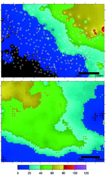
vari-ograms were, therefore, not always smooth in defini-tion. In the case of the SSM/I data, all pixels in the study region were used for each year to produce the variograms. Therefore, the variograms are “smooth” in character. Authorized models were fitted to all experi-mental variograms using a least squares criterion (Pebesma and Wesseling 1998) with the exception of the ground data for 1990 and 1991 when the experi-mental variograms were unbounded. The reason for the lack of structure for these 2 yr is probably because there was so little snow accumulated at the stations (means of 1.8 and 1.5 cm). These means are substantially com-posed of 0-cm measurements such that very little spatial variation was present. For two datasets (1996 ground and 1997 SSM/I), data were detrended using first-order polynomials; this was because a trend in the data pro-duced unbounded variograms. Unlike the 1990 and 1991 data for the ground SD measurements, appre-ciable snow accumulation was present in both 1996 and 1997, and clear-direction snow accumulation gradients were present (NE to SW in the case of the 1996 ground data and NW to SE for the SSM/I-derived SD). These directional trends were caused by the presence of syn-optic-scale variations of snow depth, which can be present at the large regional scale. As stated earlier, this research aims to test passive-microwave-derived SDs, which are calculated at the local to regional scale, so larger synoptic-scale variations are considered an un-wanted trend in the data. Figure 4 shows the SSM/I-derived SD for 1997 and kriging interpolation of ground-measured snow depth for 1996, based on the variogram derived using the method below. The SSM/ I-derived SD data reveal a northwest to southeast trend, while the ground-measured data reveal a south-west to northeast trend of snow depth.
The main parameters of interest for the comparative analysis were the nugget variance and the range. Vari-ograms were computed and estimated to a maximum lag of 1000 km at 25-km lag separations (the support of the SSM/I data). Spherical variogram models were fit-ted to the variograms using the weighfit-ted least squares criterion. Table 2 shows the model ranges and nugget variances for the ground and the satellite snow depth dataset. The mean values are also shown. Note that the SSM/I means are area integrated and are different from the means of the ground-measured SD, which are the means of sparsely distributed snow depth measure-ments. The variograms for the SSM/I and ground SD data for each of the 10 days show some broad simi-larity with respect the mean snow depths for each year. For example, the nugget variance increases with in-creasing mean snow depth for both datasets, suggesting that representation of microscale effects of snow distri-bution is not possible for thicker snowpacks. The range decreases with increased mean snow depth in both ground and SSM/I datasets, also suggesting that snow depth variability is smaller over short distances only
FIG. 3. Variograms of (a) ground measurements of snow depth and (b) SSM/I estimates of snow depth for the Red River basin for 12 Feb 1988.
when the snow is thick. For shallower snowpacks, the spatial variability is small over comparatively larger dis-tances.
With respect to differences in variogram structure between ground- and satellite- derived snow depth data, four variogram pairs (SSM/I-derived and ground-measured) have range differences less than 200 km, one pair has a range difference between 200 and 300 km, two have differences between 300 and 400 km, and one pair has a difference between 400 and 500 km. Further-more, applying the paired t test to the SSM/I and ground SD variogram range data in Table 2 gives a|t| value of 0.32, and the critical t value for a sample of 8 is 2.37. These results suggest that there is an overall gen-eral agreement between the spatial correlation length of SD derived from the SSM/I retrievals and ground measurements for the 10-yr period. This agreement
re-flects the fact that in both datasets the range tends to be larger for shallower snowpacks while it is smaller for thicker snowpacks. However, it should be noted that this is a generalized pattern and that there are differ-ences in spatial correlation lengths between ground SD measurements and SSM/I SD estimates at the interan-nual scale. The range differences are probably caused by the differences in snow accumulation processes act-ing at the local scale (e.g., snow redistribution) that affect point measurements made by a ruler and those acting at a local to regional scale (e.g., development of complex stratigraphy) that affect the snowpack micro-wave responses.
c. Error analysis and determination of the required sampling procedures of ground snow depth measurements
Before determining how many point snow depth measurements are needed to achieve a specified SD areal accuracy, it is necessary to understand the error characteristics of satellite-derived SD and ground SD measurements. Data from both SD sources are subject to systematic and nonsystematic or random errors. For ground SD measurements, there might be both system-atic and random errors associated with each measure-ment. Systematic errors from ground-measurement data are attributed to the situation of the ruler and its representativity of the local conditions (Goodison et al. 1981). Ideally, several measurements are needed to produce a representative sample, but such information is usually not available in the cooperative data archive so that inferences about ground systematic errors can-not be made. For satellite SD data, both systematic and random errors are associated with the retrieval algo-rithm and are referred to as retrieval errors (Bell et al. 1990). Systematic biases are known to exist in relation to vegetation cover and snowpack parameterization of the algorithms. While the quantification of these errors is the focus of ongoing studies (e.g., see Derksen et al. 2003), in general, the error biases are consistent as con-firmed by the results in Table 1. For the satellite SD derivations, therefore, we assume a constant systematic error because the study location and the study date each year are constant. In this study, therefore, the er-ror term in both datasets that we use to determine the accuracy achievable from a predefined number of ground SD points is the random error term of the total error.
A technique for estimating the random error of rain-fall estimates, described in Chang et al. (1993), requires a pair of independent variables (i.e., precipitation gauge measurements and satellite estimates). Applying their methodology to snow depth retrievals, ground SD estimates and satellite-derived SD values are denoted as g and s, respectively, and it is assumed that there are random errors associated with these estimates. Thus, we can write
FIG. 4. Snow depth estimates from ground interpolated data for (top) 10 Feb 1996 using a simple inverse distance weighted inter-polation routine and from (bottom) SSM/I SD estimates for 10–12 Feb 1997. The circles in the top panel represent the locations of ground point measurements.
Fig 4 live 4/C
g⫽具g典⫹ egcm,
s⫽具s典⫹ escm, 共4兲
where具 典 represent ensemble averaging over different number of ground SD categories, and egand esare the
random errors associated with independent SD esti-mates of the ground and satellite variables. Assuming that the estimates are unbiased with uncorrelated er-rors,
具eg典⫽具es典⫽ 0 and
具eges典⫽ 0. 共5兲
The error terms egand escontain errors due to ground
point sampling and satellite retrievals from the ensem-ble averaging. We can express the mean square differ-ence of ground measurements and satellite estimates as
具共g⫺ s兲2典⫽共具g典⫺具s典兲2⫹具共e g⫺ es兲
2典cm2. 共6兲
Equation (6) states the mean square difference be-tween the ground SD and satellite-derived SD values is the variance due to the random error.
For the 10-yr dataset (1988–97), 1°⫻ 1° grid cells of latitude and longitude (approximately 104 km2) were used as the study framework to investigate the random errors. The center of each grid cell was located at every half degree of latitude and longitude with the origin of each grid cell located at the southwest corner. All grid cells were classified according to the number of point ground SD measurements within the cell, a measure of the spatial density of SD sites. To ensure that no forest cover was included in the analysis, using a map of forest cover identified in Foster et al. (1997), any 1°⫻ 1° grid cell containing a forest fraction greater than 1% was discarded. The frequency distribution of sites per cell varied from 1 SD site to 10 SD sites per cell and is plotted in Fig. 5. The most frequent category was three SD sites per cell, which had 159 cells. Typically 22 SSM/I SD retrieval points were located within each
TABLE2. Variogram characteristics of ground-measured SD and SSM/I-retrieved snow depth data. Note SSM/Iare area averages rather than the paired averages shown in Table 1.
Ground data SSM/I data Difference
Year Ground (cm) Range a (km) Nugget c0 (cm2) SSM/I (cm) Range a (km) Nugget c0 (cm2) Absolute range difference (km) 1988 23.1 863 116.0 17.5 389 5.3 474 1989 16.3 836 1.0 13.8 595 2.5 241
1990 1.8 N/A N/A 5.2 952 2.0 N/A
1991 1.5 N/A N/A 11.5 1040 3.4 N/A
1992 6.7 459 3.3 12.6 776 5.0 317 1993 19.5 727 61.8 26.9 667 0.0 60 1994 39.1 365 45.7 17.7 533 0.8 168 1995 10.3 756 7.3 22.6 563 2.1 193 1996 20.3 645 54.1 26.5 541 0.0 104 1997 45.4 334 245.8 35.9 662 24.5 328
1°⫻ 1° grid cell and linearly averaged to produce a cell mean.
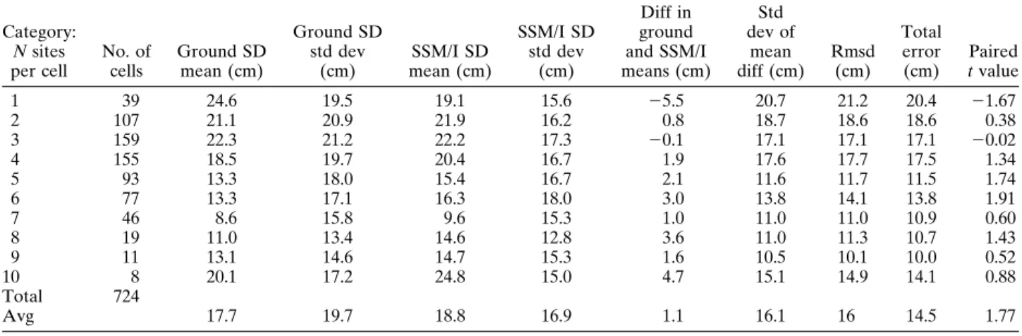
Table 3 shows the number of cells with N ground SD sites, the mean and standard deviation of ground SD and satellite SD, the mean difference between the ground SD and satellite SD (mean difference ⫽ 具g典 ⫺ 具s典) and the standard deviation of the differences, the root-mean-square of the difference (rmsd) between ground and satellite SD [rmsd⫽ 具(g ⫺ s)2典1/2]. By
re-arranging Eq. (6) above, the total error (具(eg⫺ es)典) was
calculated and is also shown in Table 3. The total error can also be written as
具e2典1Ⲑ2⫽共具eg 2
典⫹具es 2
典兲1Ⲑ2cm. 共7兲
The paired t statistic of the means was also computed. Overall, in Table 3, the mean difference and rmsd between ground and satellite SD was 1.1 and 16.0 cm, respectively. The mean difference between ground SD and SSM/I SD for each category is relatively small. From the paired t test, none of the |t| values were greater than 1.96, suggesting there was no significant difference between the mean ground and satellite-de-rived SD values. Additionally, the standard deviation of the mean difference (16.1 cm) is about the same as the mean of satellite and ground SD for each category (18.2 cm). An important characteristic of these data is that the rmsd decreases as the number of ground SD sites per cell increases, suggesting that the number of sites within a box might influence estimated random error. The total error decreases from 20.4 cm for one ground SD site to 10.0 cm at nine sites, supporting the possi-bility that the number of SD sites might influence the estimated error.
Figure 6 shows a series of graphs of SSM/I-derived snow depth, averaged for each 1°⫻ 1° grid cell plotted against the average snow depth from ground measure-ments. Each graph represents data for each year. The size of circles represents the number of ground samples
per cell for each year, and cells with more than five ground measurements are shaded gray. The diagonal line represents 100% agreement between SSM/I and ground data. For 1988, 1989, and 1996, there appears to be good agreement between datasets especially for cells with more than five ground measurements per grid cell. The unshaded circles, which have less than six sites per 1°⫻ 1° grid cell, tend to be located farther away from the line of agreement. For 1992, 1994, and 1995, the biases indicated by the mean snow depth data in Table 1 are demonstrated; for 1992 and 1995, there is an over-estimation of snow depth by the SSM/I, and in 1994 there is an underestimation. For the underestimation bias in 1994, the smaller (open) circles tend to be lo-cated within the complement of larger circles, while for the overestimation years (1992 and 1995) the smaller circles are more randomly distributed in the graphs. For 1993, the SSM/I tends to overestimate the ground-measured snow depth, although the grid cells with a greater density of ground measurements tend to be clustered. Grid cells with fewer ground sites are more widely dispersed in both graph dimensions. For 1997, the SSM/I overestimates and underestimates the snow depth (which explains why the difference between means in Table 1 is small). In general, Fig. 6 suggests that better understanding of the relationship between SSM/I estimates and ground-measured snow depth data can be obtained if a greater spatial density of ground sites is available to undertake the comparison.
The number of point measurements needed to rep-resent a physical parameter within a predefined error range depends on the spatial variability within the area and the accuracy requirements. For precipitation stud-ies, there have been several studies that addressed the sampling errors of the spatial variance of precipitation. In precipitation estimates, sampling error dominates the total error (Bell et al. 1990). Bell et al. (1990), Huff-man (1997), and Chang and Chiu (1999) reported that
TABLE3. The number of cells, mean, and standard deviation of ground SD and SSM/I SD estimates; mean difference between ground and SSM/I SD estimates, and the standard deviation of these differences; rmsd between the ground and SSM/I SD estimates; the nonsystematic errors of ground and SSM/I SD; and paired t-test value between ground and SSM/I SD for each ground SD measure-ment-site category. Category: N sites per cell No. of cells Ground SD mean (cm) Ground SD std dev (cm) SSM/I SD mean (cm) SSM/I SD std dev (cm) Diff in ground and SSM/I means (cm) Std dev of mean diff (cm) Rmsd (cm) Total error (cm) Paired t value 1 39 24.6 19.5 19.1 15.6 ⫺5.5 20.7 21.2 20.4 ⫺1.67 2 107 21.1 20.9 21.9 16.2 0.8 18.7 18.6 18.6 0.38 3 159 22.3 21.2 22.2 17.3 ⫺0.1 17.1 17.1 17.1 ⫺0.02 4 155 18.5 19.7 20.4 16.7 1.9 17.6 17.7 17.5 1.34 5 93 13.3 18.0 15.4 16.7 2.1 11.6 11.7 11.5 1.74 6 77 13.3 17.1 16.3 18.0 3.0 13.8 14.1 13.8 1.91 7 46 8.6 15.8 9.6 15.3 1.0 11.0 11.0 10.9 0.60 8 19 11.0 13.4 14.6 12.8 3.6 11.0 11.3 10.7 1.43 9 11 13.1 14.6 14.7 15.3 1.6 10.5 10.1 10.0 0.52 10 8 20.1 17.2 24.8 15.0 4.7 15.1 14.9 14.1 0.88 Total 724 Avg 17.7 19.7 18.8 16.9 1.1 16.1 16 14.5 1.77
FIG. 6. Scatterplots of SSM/I-derived snow depth against ground station snow depth for all years except 1990 and 1991 when there was little snow accumulation. The size of circles represent the number of ground measurement sites per 1°⫻ 1° grid cell. Shaded circles represent grid cells with more than five snow depth ground measurements.
the relationship between sample error of spatial vari-ance () and the number of samples is of the form 2⬃
1/n for precipitation. Rudolf et al. (1994) reported a similar error estimation relationship of the form 2 ⬃ 1/n1.11in a 2.5°⫻ 2.5° grid domain of gauge
precipita-tion data. In this snow study we attempt to determine the number of samples required for SD estimates at a 1°⫻ 1° grid domain within a limit of sampling error . To be 95% confident that the true mean is within⫾ of the observed mean, the number of samples (N ) re-quired is (Snedecor and Cochran 1967)
2⫽
共1.96兲2ⲐN ⬇ 42ⲐN, 共8兲 where is the standard deviation of the variable.
From Eq. (7), the total error具e2典1/2can be calculated
by the square root of the sum of ground SD error 具e2 g典
and satellite error 具e2
s典. The ground SD mean error is
dominated by ground-site sample configuration, espe-cially the site spatial density. The satellite error is caused by algorithm error and is not directly related to the ground-site spatial density. Since the snowfield of the NGP area is rather uniform (relatively homoge-neous low-height vegetation and snowpack properties), it is possible to make the assumption that the satellite algorithm error is probably about the same for all grid cells. By calculating es using Eq. (8) for each grid cell
category (number of ground sites per cell in Table 3), the calculated mean esfor all categories is 8.8 cm (with
a standard deviation of less than 1.0 cm). By incorpo-rating this value with the total error from Eq. (6) (also shown in Table 3), egcan be individually estimated for
each category using Eq. (8). It is then possible to opti-mize a model fit using the least squares criterion of e2
gin
proportion to 1/N. The result is e2g⫽ 466.7/N. Figure 7
shows the estimated sampling error for different num-bers of ground sites per grid cell and the fitted model. The ground SD error varies from about 20 cm for 1 site per grid cell and decreases to 7 cm for 10 sites per cell.
In other words, in order to achieve 5-cm accuracy, more than 10 ground SD measurement sites within a grid cell are required. This is an important outcome since it de-fines a limitation to the error characteristic as a func-tion of the measurement-site spatial density at this grid cell scale (i.e., 1°⫻ 1° of latitude and longitude).
5. Summary and discussion
Ten years of ground SD data were used to evaluate the single SSM/I-footprint-derived SD for northern Great Plains snowfields during midwinter. From year to year comparisons, 8 out of 20 yr had significant differ-ences between ground and SSM/I derived SD data. The mean ground SD for the 10-yr composite was 17.9 cm with a standard deviation 21.9 cm, while the SSM/I-derived SD was 18.3 cm with a standard deviation of 17.9 cm. The 10-yr mean difference between ground SD and SSM/I-derived SD was 0.4 cm, which is not statis-tically significant.
The variograms of ground SD and SSM/I derived SD were comparable. The absolute geostatistical range dif-ferences between ground SD and SSM/I SD is less than 500 km. In general, the ranges decreased as the snow depth increased, suggesting that for thinner snowpacks, the correlation lengths increase, while for thicker snow-packs they decrease. Also, the nugget variances were larger for thicker snowpacks, suggesting that there is more unresolved variation at each sample point when greater snow accumulations are present.
Comparisons of the 1°⫻ 1° latitude–longitude grid-ded data showed that the yearly differences of ground SD and SMM/I SD were not significant. The 10-yr com-posite mean and standard deviation of the ground SD was 17.7 and 19.7 cm, respectively, and the SSM/I-derived SD was 18.8 and 16.9 cm, respectively. The mean difference between ground and satellite-derived SD was 1.1 cm and was not significant. The standard deviation of the difference between ground and SSM/I SD was slightly smaller (16.1 cm) than the comparison for point data (18.7 cm).
For the composite mean of the 10-yr period, this re-search suggests that at the 1°⫻ 1° grid cell scale, SSM/I data can be used effectively to map snow depth in the NGP area. At the interannual time scale, however, there was both agreement and disagreement between ground and SSM/I-derived SD data. When the spatial density of ground SD measurements is increased, we suggest that snow depth spatial variability can be cap-tured by the SSM/I retrieval algorithm and has a calcu-lated error of 8.8 cm. In comparing the SSM/I data with ground measurements, the advantage of increasing the number of measurements sites within a grid cell is re-ported. The modeled sampling error curve of ground SD measurements is about 22 cm for 1 site, 7 cm for 10 sites, and for more than 10 sites less than 7 cm on a 1°⫻ 1° grid cell domain. This curve relating estimation
FIG. 7. Estimated ground SD error vs number of SD measurement sites.
error with number of measurements sites per cell shows that for the northern Great Plains area, the sampling error does not reduce quickly, even as the number of ground SD sites approaches 10. In the context of global snow depth estimates, this research demonstrates that it is rather difficult to quantify the global SD accuracy by using only the limited ground SD data where measure-ment-site density is often less than one per 1° ⫻ 1° of latitude and longitude. Perhaps, therefore, the only way to use these spatially limited datasets is to scale up (average) both the passive microwave data and the ground measurements to a grid cell size that is in excess of 1° ⫻ 1° of latitude and longitude. Even then, in certain parts of the world where ground data are very sparse, comprehensive validation of passive microwave estimates of snow depth may not be possible without a dedicated ground or aircraft field campaign.
The Advanced Microwave Scanning Radiometer (AMSR) was launched on board the Japanese
Ad-vanced Earth Observing Satellite-II (ADEOS-II) and
the U.S. Earth Observation System (EOS) Aqua satel-lite in 2002. AMSR can provide the best ever spatial resolution multifrequency passive microwave radiom-eter observations from space [18-GHz channel instan-taneous field of view (IFOV) is 27 ⫻ 16 km2and 36-GHz channel IFOV is 14 ⫻ 8 km2]. This capability
provides us with an opportunity to estimate surface snow mass quantities at finer spatial resolutions than have been possible with previous microwave instru-ments and so is an opportunity to improve snow depth observations both with respect to spatial resolution and accuracy of retrieval. However, for field experiments designed to test satellite observations, the ground-sampling network requires careful planning to ensure snow cover parameters such as SD are accurately mea-sured.
Acknowledgments. We thank three anonymous
ref-erees for their most helpful and insightful comments. We are also grateful to the editor of the Journal of
Hydrometeorology for his valuable assistance.
REFERENCES
Armstrong, R. L., and M. Brodzik, 1995: An earth-gridded SSM/I data set for cryospheric studies and global change monitor-ing. Adv. Space Res., 10, 155–163.
——, and ——, 2001: Recent Northern Hemisphere snow extent: A comparison of data derived from visible and microwave satellite sensors. Geophys. Res. Lett., 28, 3673–3676. ——, and ——, 2002: Hemispheric-scale comparison and
evalua-tion of passive-microwave snow algorithms. Ann. Glaciol., 34, 38–44.
Atkinson, P. M., 1993: The effect of spatial resolution on the experimental variogram of airborne MSS imagery. Int. J.
Re-mote Sens., 14, 1005–1011.
——, and R. E. J. Kelly, 1997: Scaling-up point snow depth data in the U.K. for comparison with SSM/I imagery. Int. J. Remote
Sens., 18, 437–443.
Bell, T. L., A. Abdullah, R. L. Martin, and G. R. North, 1990:
Sampling errors for satellite-derived tropical rainfall: Monte Carlo study using a space–time stochastic model. J. Geophys.
Res., 95, 2195–2205.
Brasnett, B., 1999: A global analysis of snow depth for numerical weather prediction. J. Appl. Meteor., 38, 726–740.
Brown, R., B. Brasnett, and D. Robinson, 2003: Gridded North American monthly snow depth and snow water equivalent for GCM evaluation. Atmos.–Ocean, 41, 1–14.
Chang, A. T. C., and L. S. Chiu, 1999: Nonsystematic errors of monthly oceanic rainfall derived from SSM/I. Mon. Wea.
Rev., 127, 1630–1638.
——, J. L. Foster, and D. K. Hall, 1987: Nimbus-7 derived global snow cover parameters. Ann. Glaciol., 9, 39–44.
——, L. S. Chiu, and T. T. Wilheit, 1993: Random errors of oce-anic monthly rainfall derived from SSM/I using probability distribution functions. Mon. Wea. Rev., 121, 2351–2354. Colbeck, S. C., 1982: An overview of seasonal snow
metamor-phism. Rev. Geophys. Space Phys., 20, 45–61.
Derksen, C., E. LeDrew, A. Walker, and B. Goodison, 2002: Time-series analysis of passive microwave derived central North American snow water equivalent (SWE) imagery.
Ann. Glaciol., 34, 1–7.
——, Walker, and B. Goodison, 2003: A comparison of 18 winter seasons of in situ and passive microwave-derived snow water equivalent estimates in western Canada. Remote Sens.
Envi-ron., 88, 271–282.
Foster, J. L., A. T. C. Chang, and D. K. Hall, 1997: Comparison of snow mass estimates from a prototype passive microwave snow algorithm, a revised algorithm and snow depth clima-tology. Remote Sens. Environ., 62, 132–142.
Frei, A., and D. A. Robinson, 1999: Northern Hemisphere snow extent: Regional variability 1972–1994. Int. J. Climatol., 19, 1535–1560.
Goita, K., A. Walker, and B. Goodison, 2003: Algorithm devel-opment for the estimation of snow water equivalent in the boreal forest using passive microwave data. Int. J. Remote
Sens., 24, 1097–1102.
Goodison, B. E., and A. E. Walker, 1995: Canadian development and use of snow cover information from passive microwave satellite data. Passive Microwave Remote Sensing of Land–
Atmosphere Interactions, B. Choudhury et al., Eds., VSP
Press, 245–262.
——, H. L. Ferguson, and G. A. McKay, 1981: Measurement and data analysis. Handbook of Snow: Principles, Processes,
Man-agement and Use, D. M. Gray and D. H. Male, Eds.,
Perga-mon Press, 191–274.
——, B. Sevruk, and S. Klemm, 1989: WMO solid precipitation measurement intercomparison: Objectives, methodology, analysis. Atmospheric Deposition, J. W. Delleur, Ed., IAHS Publication 179, 57–64.
Huffman, G. J., 1997: Estimates of root-mean-square random er-ror for finite samples of estimated precipitation. J. Appl.
Me-teor., 36, 1191–1201.
Isaaks, E. H., and R. M. Srivastava, 1989: Applied Geostatistics. Oxford University Press, 580 pp.
Jacobson, M. Z., 1999: Fundamentals of Atmospheric Modeling. Cambridge University Press, 656 pp.
Josberger, E. G., and N. M. Mognard, 2002: A passive microwave snow depth algorithm with a proxy for snow metamorphism.
Hydrol. Processes, 16, 1557–1568.
——, P. Gloersen, A. Chang, and A. Rango, 1996: The effects of snowpack grain size on satellite passive microwave observa-tions from the upper Colorado River basin. J. Geophys. Res.,
101 (C3), 6679–6688.
——, N. M. Mognard, B. Lind, R. Matthews, and T. Carroll, 1998: Snowpack water-equivalent estimates from satellite and air-craft remote-sensing measurements of the Red River basin, north-central U.S.A. Ann. Glaciol., 26, 119–124.
Kelly, R. E. J., A. T. C. Chang, L. Tsang, and J. L. Foster, 2003: Development of a prototype AMSR-E global snow area and
snow volume algorithm. IEEE Trans. Geosci. Remote Sens.,
41, 230–242.
Matzler, C., 1987: Applications of the interaction of microwave with the natural snow cover. Remote Sens. Rev., 2, 259–387. McClave, J. T., and F. H. Dietrich II, 1979: Statistics. Dellen, 681
pp.
Mognard, N. M., and E. G. Josberger, 2002: Northern Great Plains 1996/97 seasonal evolution of snowpack parameters from passive microwave measurements. Ann. Glaciol., 34, 15–23.
Pebesma, E. J., and C. G. Wesseling, 1998: GSTAT, a program for geostatistical modeling, prediction and simulation. Comput.
Geosci., 24, 17–31.
Rudolf, B., H. Hauschild, W. Rueth, and U. Schneider, 1994: Ter-restrial precipitation analysis: Operational method and re-quired density of point measurements. Global Precipitation
and Climate Change, M. Desbois and F. Desalmand, Eds.,
NATO ASI Series, Vol. 126, Springer-Verlag, 173–186.
Snedecor, G. W., and W. G. Cochran, 1967: Statistical Methods. 6th ed. Iowa State University Press, 593 pp.
Stiles, W. H., and F. T. Ulaby, 1980: The active and passive mi-crowave response to snow parameters. 1. Wetness. J.
Geo-phys. Res., 85, 1037–1044.
Walker, A. E., and A. Silis, 2001: Snow cover variations over the Mackenzie River basin derived from SSM/I passive micro-wave satellite data. Ann. Glaciol., 34, 8–14.
Yang, D., B. Goodison, S. Ishida, and C. Benson, 1998: Adjust-ment of daily precipitation data at 10 climate stations in Alaska: Application of World Meteorological Organization intercomparison results. Water Resour. Res., 34, 241–256. ——, and Coauthors, 1999: Quantification of precipitation
mea-surement discontinuity induced by wind shields on national gauges. Water Resour. Res., 35, 491–508.
——, and Coauthors, 2000: An evaluation of the Wyoming gauge system for snowfall measurement. Water Resour. Res., 36, 2665–2677.