HAL Id: hal-00003139
https://hal.archives-ouvertes.fr/hal-00003139
Submitted on 21 Nov 2019
HAL is a multi-disciplinary open access
archive for the deposit and dissemination of
sci-entific research documents, whether they are
pub-lished or not. The documents may come from
teaching and research institutions in France or
abroad, or from public or private research centers.
L’archive ouverte pluridisciplinaire HAL, est
destinée au dépôt et à la diffusion de documents
scientifiques de niveau recherche, publiés ou non,
émanant des établissements d’enseignement et de
recherche français ou étrangers, des laboratoires
publics ou privés.
quantum spin models
Sylvain Capponi, Andreas Laeuchli, Matthieu Mambrini
To cite this version:
Sylvain Capponi, Andreas Laeuchli, Matthieu Mambrini.
Numerical contractor renormalization
method for quantum spin models. Physical Review B: Condensed Matter and Materials Physics
(1998-2015), American Physical Society, 2004, 70 (10), pp.104424. �10.1103/PhysRevB.70.104424�.
�hal-00003139�
an effective Hamiltonian with longer ranged interactions up to a certain cutoff using the CORE algorithm and
(ii) solving this new model numerically on finite clusters by exact diagonalization and performing finite-size
extrapolations to obtain results in the thermodynamic limit. This approach, giving complementary information to analytical treatments of the CORE Hamiltonian, can be used as a semiquantitative numerical method. For ladder-type geometries, we explicitely check the accuracy of the effective models by increasing the range of the effective interactions until reaching convergence. Our results in the perturbative regime and also away from it are in good agreement with previously established results. In two dimensions we consider the plaquette lattice and the kagomé lattice as nontrivial test cases for the numerical CORE method. As it becomes more difficult to extend the range of the effective interactions in two dimensions, we propose diagnostic tools(such as the density matrix of the local building block) to ascertain the validity of the basis truncation. On the plaquette lattice we have an excellent description of the system in both the disordered and the ordered phases, thereby showing that the CORE method is able to resolve quantum phase transitions. On the kagomé lattice we find that the previously proposed twofold degenerate S = 1 / 2 basis can account for a large number of phenom-ena of the spin 1 / 2 kagomé system. For spin 3 / 2, however, this basis does not seem to be sufficient. In general we are able to simulate system sizes which correspond to an 8⫻8 lattice for the plaquette lattice or a 48-site
kagomé lattice, which are beyond the possibilities of a standard exact diagonalization approach.
DOI: 10.1103/PhysRevB.70.104424 PACS number(s): 75.10.Jm, 75.40.Mg, 75.40.Cx
I. INTRODUCTION
Low-dimensional quantum magnets are at the heart of current interest in strongly correlated electron systems. These systems are driven by strong correlations and large quantum fluctuations—especially when frustration comes into play— and can exhibit various unconventional phases and quantum phase transitions.
One of the major difficulties in trying to understand these systems is that strong correlations often generate highly non-trivial low-energy physics. Not only is the ground state of such models generally not known but also the low-energy degrees of freedom cannot be easily identified. Moreover, among the techniques available for investigating these sys-tems, not many have the required level of generality to pro-vide a systematic way to derive low-energy effective Hamil-tonians.
Recently the contractor renormalization(CORE) method was introduced by Morningstar and Weinstein.1The key idea
of the approach is to derive an effective Hamiltonian acting on a truncated local basis set, so as to exactly reproduce the low energy spectrum. In principle the method is exact in the low-energy subspace, but only at the expense of having a
priori long range interactions. The method becomes most
useful when one can significantly truncate a local basis set and still restrict oneself to short range effective interactions. This, however, depends on the system under consideration and has to be checked systematically. Since its inception the CORE method has been mostly used as an analytical method to study strongly correlated systems.2–4 Some first steps in
using the CORE approach and related ideas in a numerical framework have also been undertaken.5–8
The purpose of the present paper is to explore the numeri-cal CORE method as a complementary approach to more analytical CORE procedures, and to systematically discuss its performance in a variety of low-dimensional quantum magnets, both frustrated and unfrustrated. The approach con-sists basically of numerical exact diagonalizations of the ef-fective Hamiltonians. In this way a large number of interest-ing quantities are accessible, which otherwise would be hard to obtain. Furthermore, we discuss some criteria and tools useful to estimate the quality of the CORE approach.
The outline of the paper is as follows: In Sec. II we will review the CORE algorithm in general and discuss some particularities in a numerical CORE approach, both at the level of the calculation of the effective Hamiltonians and the subsequent simulations.
In Sec. III we move to the first applications on one-dimensional(1D) systems: the well-known two-leg spin lad-der and the three-leg spin ladlad-der with periodic boundary con-ditions in the transverse direction (three-leg torus). Both systems exhibit, generically, a finite spin gap and a finite magnetic correlation length. We will show that the numerical CORE method is able to get rather accurate estimates of the ground state energy and the spin gap by successively increas-ing the range of the effective interactions.
In Sec. IV we discuss two-dimensional(2D) systems. Be-cause in 2D a long-ranged cluster expansion of the interac-tions is difficult to achieve, we will discuss some techniques to analyze the quality of the basis truncation. We illustrate these issues on two model systems, the plaquette lattice and the kagomé lattice. The plaquette lattice is of particular in-terest as it exhibits a quantum phase transition from a disor-dered plaquette state to a long-range ordisor-dered Néel
magnet, which cannot be reached by a perturbative approach. We show that a range-two effective model captures many aspects of the physics over the whole range of parameters. The kagomé lattice on the other hand is a highly frustrated lattice built of corner-sharing triangles. For spin 1/2 it has been studied both numerically and analytically and it is one of the best-known candidate systems for a spin liquid ground state. A very peculiar property is the exponentially large number of low-energy singlets in the magnetic gap. We show that already a basic range two CORE approach is able to devise an effective model which exhibits the same exotic low-energy physics. For higher half-integer spin, i.e., S = 3 / 2, this simple effective Hamiltonian breaks down; we analyze how to detect this, and discuss some ways to im-prove the results.
In Sec. V we conclude and give some perspectives. Fi-nally three appendices are devoted to(i) the density matrix of local building block,(ii) the calculation of observables by energy considerations, and(iii) some general remarks on ef-fective Hamiltonians coupling antiferromagnetic half-integer spin triangles.
II. CORE ALGORITHM
The contractor renormalization(CORE) method has been proposed by Morningstar and Weinstein in the context of general Hamiltonian lattice models.1Later, Weinstein applied
this method with success to various spin chain models.2For a review of the method we refer the reader to these original papers1,2 and also to a pedagogical article by Altman and
Auerbach3which includes many details. Here, we summarize
the basic steps before discussing some technical aspects which are relevant in our numerical approach.
CORE Algorithm:
(1) Choose a small cluster (e.g., rung, plaquette, triangle, etc.) and diagonalize it. Keep M suitably chosen low-energy states.
(2) Diagonalize the full Hamiltonian H on a connected graph consisting of Nc clusters and obtain its low-energy
states兩n典 with energies n.
(3) The eigenstates兩n典 are projected on the tensor product space of the states kept and Gram-Schmidt orthonormalized in order to get a basis 兩n典 of dimension MNc. As it may
happen that some of the eigenstates have zero or very small projection, or vanish after the orthogonalization it might be necessary to explicitely compute more than just the lowest
MNceigenstates兩n典.
(4) Next, the effective Hamiltonian for this graph is built as
hNc=
兺
n=1 MNcn兩n典具n兩. 共1兲
(5) The connected range-Nc interactions hNc
conn are
deter-mined by substracting the contributions of all connected sub-clusters.
(6) Finally, the effective Hamiltonian is given by a cluster expansion as HCORE=
兺
i hi+兺
具ij典 hij+兺
具ijk典 hijk+ ¯ . 共2兲This effective Hamiltonian exactly reproduces the low-energy physics provided the expansion goes to infinity. How-ever, if the interactions are short-range in the starting Hamil-tonian, we can expect that these operators will become smaller and smaller, at least in certain situations. In the fol-lowing, we will truncate at range r and verify the conver-gence in several cases. This converconver-gence naturally depends on the number M of low-lying states that are kept on a basic block. In order to describe quantitatively how “good” these states are, we introduce the density matrix in Sec. IV.
When the number of blocks increases, a full diagonaliza-tion is not always easy and one is tempted to use a Lanczos algorithm in order to compute the low-lying eigenstates. In that case, one has to be very careful to resolve the correct degeneracies, which is known to be a difficult task in the Lanczos framework. In practice such degeneracies arise when the cluster to be diagonalized is highly symmetric. If the degeneracies are ignored, often a wrong effective Hamil-tonian with broken SU(2) symmetry is obtained. As a conse-quence we recommend to use specialized LAPACK routines whenever possible.
In the present work we investigate mainly SU(2) invariant Heisenberg models described by the usual Hamiltonian
H =
兺
具ij典JijSi· Sj, 共3兲
where the exchange constants Jij will be limited to
short-range distances in the following. As a consequence of the SU(2) symmetry, the total spin of all states is a good quan-tum number. This also has some effects when calculating the effective Hamiltonian. It is possible to have situations where a low energy state has a nonzero overlap with the tensor product basis, but gets eliminated by the orthogonalization procedure because one has already exhausted all the states in one particular total spin sector by projecting states with lower energy.
Once an effective Hamiltonian has been obtained, it is still a formidable task to determine its properties. Within the CORE method different routes have been taken in the past. In their pioneering papers Morningstar and Weinstein have chosen to iteratively apply the CORE method on the preced-ing effective Hamiltonian in order to flow to a fixed point and then to analyze the fixed point. A different approach has been taken in Refs. 3 and 4: There the effective Hamiltonian after one or two iterations has been analyzed with mean-field like methods and interesting results have been obtained. Yet another approach—and the one we will pursue in this paper—consists of a single CORE step to obtain the effective Hamiltonian, followed by a numerical simulation thereof. This approach has been explored in a few previous studies.5–7The numerical technique we employ is the exact diagonalization (ED) method based on the Lanczos algo-rithm. This technique has easily access to many observables and profits from the symmetries and conservation laws in the problem, i.e., total momentum and the total Sz component.
of dimensions up to⬃50 million, however the matrices con-tain significantly more matrix elements than the ones of the microscopic Hamiltonian we start with.
III. LADDER GEOMETRIES
In this section, we describe results obtained on ladder systems with 2 and 3 legs, respectively.
We want to build an effective model that is valid from a perturbative regime to the isotropic case Jij= J = 1. We have
chosen periodic boundary conditions(PBC) along the chains in order to improve the convergence to the thermodynamic limit.
A. Two-leg Heisenberg ladder
The 2-leg Heisenberg ladder has been intensively studied and is known to exhibit a spin gap for all couplings.9,10
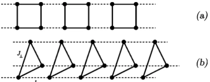
In order to apply our algorithm, we select a 2⫻2 plaquette as the basic unit[see Fig. 1(a)]. The truncated sub-space is formed by the singlet ground-state (GS) and the lowest triplet state.
Using the same CORE approach, Piekarewicz and Shep-ard have shown that quantitative results can be obtained within this restricted subspace.5 Moreover, dynamical
quan-tities can also be computed in this framework.6
Since we are dealing with a simple system, we can com-pute the effective models including rather long-range inter-actions(typically, to obtain range-4 interactions, we need to compute the low-lying states on a 2⫻8 lattice with open boundary conditions which is feasible, although it requires a large numerical effort). It is desirable to compute long-range effective interactions since we wish to check how the trun-cation affect the physical results and how the convergence is reached.
In a second step, for each of these effective models, we perform a standard exact diagonalization (ED) using the Lanczos algorithm on finite clusters up to Nc= 12 clusters
(N=48 sites for the original model). The GS energy and the spin gap are shown in Fig. 2. The use of PBC allows us to reduce considerably finite-size effects since we have an ex-ponential convergence as a function of inverse length. CORE results are in perfect agreement with known results and the successive approximations converge uniformly to the exact results. For instance, the relative errors of range-4 results are 10−4for the GS energy and 10−2 for the spin gap. This fast
convergence is probably due to the rather short correlation
length in an isotropic ladder (typically 3–4 lattice spacings11).
B. 3-leg Heisenberg torus
As a second example of ladder geometry, we have studied a 3-leg Heisenberg ladder with PBC along the rungs. This property causes geometric frustration which leads to a finite spin-gap and finite dimerization for all interchain coupling
J⬜,12,13contrary to the open boundary condition case along
the rungs, which is in the universality class of the Heisenberg chain.
1. Perturbation theory
The simple perturbation theory is valid when the coupling along the rung 共J⬜兲 is much larger than between adjacent rungs共J储兲. In the following, we fix J⬜= 1 as the energy unit and denote␣= J储/ J⬜.
On a single rung, the low-energy states are the following degenerate states, defined as
兩↑L典 =
冑
1 3共兩↑↑↓典 +兩↑↓↑典 + 2兩↓↑↑典兲, 兩↓L典 =冑
1 3共兩↓↓↑典 +兩↓↑↓典 + 2兩↑↓↓典兲, 兩↑R典 =冑
1 3共兩↑↑↓典 + 2兩↑↓↑典 +兩↓↑↑典兲, 兩↓R典 =冑
1 3共兩↓↓↑典 + 2兩↓↑↓典 +兩↑↓↓典兲, 共4兲where = exp共i2/ 3兲. The indices L and R represent the momentum of the 3-site rung ky= 2/ 3 and −2/ 3,
respec-tively. They define two chiral states which can be viewed as
FIG. 1. (a) 2-leg ladder. Basic block is a 2⫻2 plaquette. (b) 3-leg torus with rung coupling J⬜and inter-rung coupling J储.
FIG. 2. Ground-state energy per site and spin gap of a 2⫻L
Heisenberg ladder using CORE method with various range r using PBC. For comparison, we plot the best known extrapolations(Ref. 10) with arrows.
pseudo-spin states with operators on each rung defined by +兩·R典 = 0, +兩·L典 = 兩·R典, −兩·R典 = 兩·L典, −兩·L典 = 0, z兩·R典 =1 2兩·R典, z兩·L典 = −1 2兩·L典.
These states have in addition a physical spin 1/2 described by.
Applying the usual perturbation theory for the inter-rung coupling, one finds12,14
Hpert= − N 4 + ␣ 3
兺
具ij典i·j共1 + 4共i + j − +i−j+兲兲, 共5兲where N is the total number of sites.
This effective Hamiltonian has been studied with DMRG and ED techniques and it exhibits a finite spin gap ⌬S
= 0.28 J储and a dimerization of the ground state.12,13
Here we want to use the CORE method to extend the perturbative Hamiltonian with an effective Hamiltonian in the same basis for any coupling.
2. CORE approach
As a basic unit, we choose a single 3-site rung. The sub-space consists of the same low-energy states as for the per-turbative result [Eq. (4)] which are fourfold degenerate (2 degenerate S = 1 / 2 states). We can apply our procedure to compute the effective interactions at various ranges, in order to be able to test the convergence of the method.
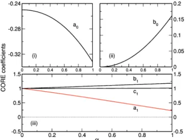
First, we write down the range-2 contribution under the most general form which preserves both SU共2兲 (spin) sym-metry and simultaneous translation or reflection along all the rungs: Hr=2= Na0+
兺
具ij典共b0i z j z + c0共i + j − +i−+j兲兲 +i·j共a1+ b1i z j z + c1共i + j − +i−+j兲兲. 共6兲 In the perturbative regime given in(5), the only nonvan-ishing coefficients are given by: a0= −1 / 4, a1=␣/ 3, and c1= 4␣/ 3.
The parameters of the effective Hamiltonian can be ob-tained and their dependence as a function of the inter-rung coupling ␣ is shown in Fig. 3. We immediately see some deviations from the perturbative result since coefficients in panel(i) and (ii) are nonzero and become as important as the other terms in the isotropic limit. Surprisingly, we observe that c1follows its perturbative expression on the whole range
of couplings whereas a1deviates strongly as one goes to the
isotropic case but does not change sign.
In order to study how the physical properties evolve as a function of J储/ J⬜, we have computed the GS energy and the spin gap both for a small-coupling case and in the isotropic limit, up to range 5 in the effective interactions.
3. Small inter-rung coupling
We have chosen J储/ J⬜= 0.25 which corresponds to a case where perturbation theory should still apply. Using ED, we
can solve the effective models on finite lattices and in Fig. 4, we plot the scaling of the GS energy and of the spin gap as a function of the system length L. Even for this rather small value of J储/ J⬜, our effective Hamiltonian can be considered
as an improvement over the first order perturbation theory. Moreover, we observe a fast convergence with the range of interactions and already the range-3 approximation is almost indistinguishable from ED results.
The estimated gap is 0.16J储 and correspond to a lower
bound since ultimately the gap should converge exponen-tially to its thermodynamic value. Our value is consistent with the DMRG one12共⬃0.2J
储兲, and is already reduced
com-pared to the strong coupling result12共⌬
S= 0.28J储兲. 4. Isotropic case
We apply the same procedure in the isotropic limit. As expected, the convergence with the range of interactions is much slower than in the perturbative regime. We show in Fig. 5 that indeed the ground state energy converges slowly and oscillates around the correct value. These oscillations come from the fact that, in order to compute range-r interac-tions, one has to study alternatively clusters with an even or odd number of sites. Since this system has a tendency to form dimers on nearest-neighbor bonds, it is better to com-pute clusters with an even number of sites.
For the spin gap, we find accurate results even with lim-ited range interactions. In particular, we find that frustration induces a finite spin gap⯝0.11 J储 in that system. As in the previous case, this is a lower bound which is in perfect agreement with DMRG study.12
Moreover, we observe that the singlet gap vanishes in the thermodynamic limit as 1 / L2 (data not shown), similar to a
related study.13This singlet state at momentum along the chains corresponds to the state built in the generalized Lieb-Schultz-Mattis argument.15 Here, the physical picture is a
FIG. 3. (Color online) CORE coefficients [see Eq. (6)] for two
coupled triangles as a function of the inter-rung coupling ␣
= J储/ J⬜. The parameters were computed using range-2 CORE. The coefficients in panel(iii) have been divided by their values in the perturbative limit. They therefore all start at 1.
twofold degenerate GS due to the appearance of spontaneous dimerization.
5. Spinon dispersion relation for the spin tube
One of the advantages of this method is to be able to get information on some quantum numbers(number of particles, magnetization, momentum,. . .). For example, the effective Hamiltonian Heffstill commutes with translations along the
legs, with the total Sztotandzso that we can work in a given
momentum sector共kx, ky兲 with a fixed magnetization Sz
tot. By
computing the energy in each sector, we can compute the dispersion relation.
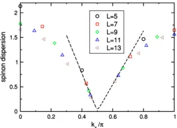
In order to try to identify if the fundamental excitation is a spinon, we compute the energy difference between the low-est S = 1 / 2 state when the length is odd共L=2p+1兲 and the extrapolated GS energy obtained from the data on systems with even length 2p and 2p + 2. The data are taken from CORE with range-4 approximation. In Fig. 6, we plot this dispersion as a function of the longitudinal momentum, rela-tive to the GS with L = 2p.
We observe a dispersion compatible with a spinonlike dis-persion, which is massive with a gap at/ 2⯝0.05⯝⌬S/ 2.
This result is consistent with a picture in which the triplet excitation⌬S is made of two elementary spinons. With our
precision, it seems that the spinons are not bound but we cannot exclude a small binding energy.
We have a good overall agreement with results obtained in the strong interchain coupling regime.13
FIG. 4. GS energy per site and spin gap for a 3⫻L Heisenberg torus with J储/ J⬜= 0.25. Results are obtained using the CORE method at various range r.
FIG. 5. Same as Fig. 4 for the isotropic case J储= J⬜= 1.
FIG. 6. (Color online) Spinon dispersion relation (see text) as a function of longitudinal momentum(in units of). We only plot the lowest branch corresponding to ky= ± 2/3. The odd lengths run from 5 to 13. The lines are guide to the eyes for an extrapolation on both sides of/2.
Therefore, with CORE method, we have both the advan-tage of working in the reduced subspace and not being lim-ited to the perturbative regime. Amazingly, we have observed that for a very small effort (solving a small cluster), the effective Hamiltonian gives much better results (often less than 1% on GS energies) than perturbation theory. It also gives an easier framework to systematically improve the ac-curacy by including longer range interactions.
For these models, the good convergence of CORE results may be due to the fact that the GS in the isotropic limit is adiabatically connected to the perturbative one. In the fol-lowing part we will therefore study 2D models where a quantum phase transition occurs as one goes from the pertur-bative to the isotropic regime.
IV. TWO-DIMENSIONAL SPIN MODELS
In this section we would like to discuss the application of the numerical CORE method to two dimensional quantum spin systems. We will present spectra and observables and also discuss a novel diagnostic tool—the density matrix of local objects—in order to justify the truncation of the local state set.
One major problem in two dimension is the more elabo-rate cluster expansion appearing in the CORE procedure. Es-pecially our approach based on numerical diagonalization of the resulting CORE Hamiltonian faces problems once the CORE interaction clusters wrap around the boundary of the finite size clusters. We therefore try to keep the range of the interactions minimal, but we still demand a reasonable de-scription of low energy properties of the system. We will therefore discuss some ways to detect under what circum-stances the low-range approximations fail and why.
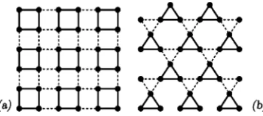
As a first example we discuss the plaquette lattice[Fig. 7(a)], which exhibits a quantum phase transition from a gapped plaquette-singlet state with only short ranged order to a long range ordered antiferromagnetic state as a function of the interplaquette coupling.16–19We will show that the CORE
method works particularly well for this model by presenting results for the excitation spectra and the order parameter. It is also a nice example of an application where the CORE method is able to correctly describe a quantum phase transi-tion, thus going beyond an augmented perturbation scheme. The second test case is the highly frustrated kagomé lat-tice[Fig. 7(b)] with noninteger spin, which has been inten-sively studied for S = 1 / 2 during the last few years.20–24 Its
properties are still not entirely understood, but some of the features are well accepted by now: There is no simple local order parameter detectable, neither spin order nor valence bond crystal order. There is probably a small spin gap present and most strikingly an exponentially growing num-ber of low energy singlets emerges below the spin gap. We will discuss a convenient CORE basis truncation which has emerged from a perturbative point of view23,25,26 and
con-sider an extension of this basis for higher noninteger spin. A. Plaquette lattice
The CORE approach starts by choosing a suitable decom-position of the lattice and a subsequent local basis truncation. In the plaquette lattice the natural decomposition is directly given by the uncoupled plaquettes. Among the 16 states of an isolated plaquette we retain the lowest singlet[K=共0,0兲] and the lowest triplet [K=共,兲]. The standard argument for keeping these states relies on the fact that they are the lowest energy states in the spectrum of an isolated plaquette.
As discussed in Appendix A, the density matrix of a plaquette in the fully interacting system gives clear indica-tions whether the basis is suitably chosen. In Fig. 8 we show the evolution of the density matrix weights of the lowest singlet and triplet as a function of the interplaquette cou-pling. Even though the individual weights change signifi-cantly, the sum of both contributions remains above 90% for all J
⬘
/ J艋1. We therefore consider this a suitable choice for a successful CORE application.A next control step consists in calculating the spectrum of two coupled plaquettes, and one monitors which states are targeted by the CORE algorithm. We show this spectrum in Fig. 9 along with the targeted states. We realize that the 16 states of our tensor product basis cover almost all the low energy levels of the coupled system. There are only two trip-lets just below the S = 2 multiplet which are missed.
FIG. 7.(a) The plaquette lattice. Full lines denote the plaquette
bonds J, dashed lines denote the inter-plaquette coupling J⬘.(b) The trimerized kagomé lattice. Full lines denote the up-triangle J bonds, dashed lines denote the down-triangle coupling J⬘. The standard
kagomé lattice is recovered for J⬘/ J = 1.
FIG. 8. (Color online) Density matrix weights of the two most important states on a strong(J-bonds) plaquette as a function of
J⬘/ J. These results were obtained by ED with the original Hamil-tonian on a 4⫻4 cluster.
In a first application we calculate the spin gap for differ-ent system sizes and couplings J
⬘
/ J. The results shown in Fig. 10 indicate a reduction of the spin gap for increasingJ
⬘
/ J. We used a simple finite size extrapolation in 1 / N in order to assess the closing of the gap. The extrapolation lev-els off to a small value for J⬘
/ J艌0.6. The appearance of a small gap in this known gapless region is a feature already present in ED calculation of the original model,19 andthere-fore not an artefact of our method. It is rather obvious that the triplet gap is not a very accurate tool to detect the quan-tum phase transition within our numerical approach. We will see later that order parameter susceptibilities are much more accurate.
It is well known that the square lattice共J
⬘
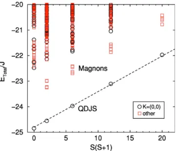
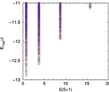
/ J = 1兲 is Néel ordered. One possibility to detect this order in ED is tocal-culate the so-called tower of excitation, i.e., the complete spectrum as a function of S共S+1兲, S being the total spin of an energy level. In the case of standard collinear Néel order a prominent feature is an alignment of the lowest level for each S on a straight line, forming a so-called “quasidegener-ate joint st“quasidegener-ates” (QDJS) ensemble,27 which is clearly
sepa-rated from the rest of the spectrum on a finite size sample. We have calculated the tower of states within the CORE approach (Fig. 11). Due to the truncated Hilbert space we cannot expect to recover the entire spectrum. Surprisingly however the CORE tower of states successfully reproduces the general features observed in ED calculations of the same model:28 (a) a set of QDJS with the correct degeneracy and
quantum numbers (in the folded Brillouin zone); (b) a re-duced number of magnon states at intermediate energies, both set of states rather well separated from the high energy part of the spectrum. While the QDJS seem not to be affected by the CORE decimation procedure, clearly some of the magnon modes get eliminated by the basis truncation.
In order to locate the quantum phase transition from the paramagnetic, gapped regime to the Néel ordered phase, a simple way to determine the onset of long range order is desirable. We chose to directly couple the order parameter to the Hamiltonian and to calculate generalized susceptibilities by deriving the energy with respect to the external coupling. This procedure is detailed in Appendix B. Its simplicity re-lies on the fact that only eigenvalue runs are necessary. Simi-lar approaches have been used so far in ED and QMC calculations.29,30
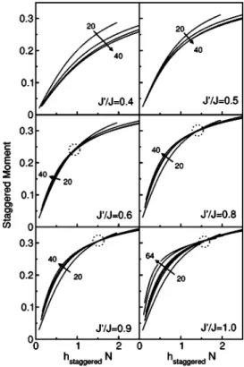
Our results in Fig. 12 show the evolution of the staggered moment per site in a rescaled external staggered field for different interplaquette couplings J
⬘
and different system sizes (up to 8⫻8 lattices). We note the appearance of an approximate crossing of the curves for different system sizes, once Néel LRO sets in. This approximate crossing relies onFIG. 9. (Color online) Low energy spectrum of two coupled
plaquettes. The states targeted by the CORE algorithm are indicated by arrows together with their SU共2兲 degeneracy.
FIG. 10. (Color online) Triplet gap for effective system sizes between 20 and 52 sites, as a function of the interplaquette coupling
J⬘/ J. For J⬘/ J艌0.5 a simple extrapolation in 1/N is also displayed. These results compare very well with ED results on the original model(Ref. 19).
FIG. 11.(Color online) Tower of states obtained with a range-2
CORE Hamiltonian on an effective N = 36 square lattice (9-site
CORE cluster) in different reduced momentum sectors. The tower of states is clearly separated from the decimated magnons and the rest of the spectrum.
the fact that the slope of mL共hN兲 diverges at least linearly in
N in the ordered phase.30 We then consider this crossing
feature as an indication of the phase transition and obtain a value of the critical point Jc/ J = 0.55± 0.05. This estimate is
in good agreement with previous studies using various methods.17–19We have checked the present approach by
per-forming the same steps on the two leg ladder discussed in Sec. III A and there was no long range magnetic order present, as expected.
B. Kagomé systems with half-integer spins
In the past 10 years many efforts have been devoted to understand the low energy physics of the kagomé antiferro-magnet(KAF) for spins 1/2.20–24At the theoretical level, the
main motivation comes from the fact that this model is the only known example of a two-dimensional Heisenberg spin liquid. Even though many questions remain open, some very exciting low-energy properties of this system have emerged. Let us summarize them briefly: (i) the GS is a singlet 共S = 0兲 and has no magnetic order. Moreover no kind of more exotic ordering (dimer-dimer, chiral order, etc.) have been detected using unbiased methods;(ii) the first magnetic ex-citation is a triplet共S=1兲 separated from the GS by a rather small gap of order J / 20;(iii) more surprisingly the spectrum
appears as a continuum of states in all spin sectors. In par-ticular the spin gap is filled with an exponential number of singlet excitations:Nsinglets⬃1.15N;(iv) the singlet sector of
the KAF can be very well reproduced by a short-range reso-nating valence bond approach involving only nearest-neighbor dimers.
From this point of view, the spin 1/2 KAF with its highly unconventional low-energy physics appears to be a very sharp test of the CORE method. The case of higher half-integer spins S = 3 / 2 , 5 / 2 , . . . KAF is also of particular inter-est, since it is covered by approximative experimental realizations.31 Even if some properties of these experimental
systems are reminiscent of the spin 1/2 KAF theoretical sup-port is still lacking for higher spins due to the increased complexity of these models.
In this section we discuss in detail the range-two CORE Hamiltonians for spin 1/2 and 3/2 KAF considered as a set of elementary up-triangles with couplings J, coupled by down-triangles with couplings J
⬘
[see Fig. 7(b)]. The coupling ratio will be denoted by␣= J⬘
/ J. Before going any further into the derivation of the CORE effective Hamiltonian let us start with the conventional degenerate perturbation theory results. Note that in the perturbative regime these two approaches yield the same effective Hamiltonian.As described in Appendix C, the most general two-triangle effective Hamiltonian involving only the two spin 1/2 degrees of freedom on each triangle can be written in the following form: H = Na0共␣兲 +
兺
具i,j典共b0共␣兲i · eijj· eij+ a1共␣兲i·j + b1共␣兲i·j共i· eij兲共j· eij兲 + c1共␣兲i·j共i· eij+j· eij兲兲. 共7兲In the spirit of Mila’s approach23 for spin 1/2 the first order
perturbative Hamiltonian in ␣can easily be extended to ar-bitrary half-integer spin S:
Hpert.=␣
9i·j⫻ 共1 − 2共2S + 1兲i· ea兲共1 − 2共2S + 1兲j· eb兲 共8兲 and the coefficients of(7) in the perturbative limit are given as a1共␣兲=␣/ 9, b1共␣兲=共4␣/ 9兲共2S+1兲2, c1共␣兲=−共2␣/ 9兲共2S
+ 1兲, b0共␣兲=0, and a0共␣兲=共1/4−S共S+1兲兲/2.
1. Choice of the CORE basis
As discussed in the previous paragraph we keep the two degenerate S = 1 / 2 doublets on a triangle for the CORE basis. In analogy to the the plaquette lattice we calculate the den-sity matrix of a single triangle embedded in a 12 site kagomé lattice for both spin S = 1 / 2 and S = 3 / 2, in order to get infor-mation on the quality of the truncated basis. The results dis-played in Fig. 13 show two different behaviors: while the targeted states exhaust 95% for the S = 1 / 2 case, they cover only⬇55% in the S=3/2 case. This can be considered a first indication that the range-two approximation in this basis might break down for S⬎1/2 half integer spin, while the approximation seems to work particularly well for S = 1 / 2,
FIG. 12. Staggered moment per site as a function of the rescaled applied staggered field for the plaquette lattice and different values of J⬘/ J. Circles denote the approximate crossing point of curves for different system sizes. We take the existence of this crossing as a phenomenological indication for the presence of Néel LRO. In this way the phase transition is detected between 0.5⬍Jc⬘/ J⬍0.6, con-sistent with previous estimates. The arrows indicate curves for in-creasing system sizes: 20, 32, 36, 40 and also 52, 64 for the isotro-pic case.
thereby providing independent support for the adequacy of the basis chosen in a related mean-field study.23
We continue the analysis of the CORE basis by monitor-ing the evolution of the spectra of two coupled triangles in the kagomé geometry(cf. Fig. 22 below) as a function of the intertriangle coupling J
⬘
, as well as the states selected by the range-two CORE algorithm. The spectrum for the spin S = 1 / 2 case is shown in Fig. 14. We note the presence of a clear gap between the 16 lowest states—correctly targeted by the CORE algorithm—and the higher lying bands. This can be considered an ideal case for the CORE method. Based on this and the results of the density matrix we expect the CORE range-two approximation to work quite well.We compare these encouraging results with the spectrum for the spin S = 3 / 2 case displayed in Fig. 15. Here the situ-ation is less convincing: very rapidly 共J
⬘
/ Jⲏ0.45兲 the lowenergy states mix with originally higher lying states and the CORE method continues to target two singlets which lie high up in energy when reaching J
⬘
/ J = 1. We expect this to be a situation where the CORE method will probably not work correctly when restricted to range-two terms only.Based on the two-triangle spectra shown above we used the CORE algorithm to determine the coefficients of the gen-eral two-body Hamiltonian Eq.(7). For an independent deri-vation, see Ref. 32. The coefficients obtained this way are shown in Figs. 16 and 17 for S = 1 / 2 and S = 3 / 2, respec-tively. In the limit ␣Ⰶ1 the coefficients can be obtained from the perturbative Hamiltonian [Eq. (8)]. There are two classes of coefficients in both cases: a0and b0are zero in the perturbative limit, i.e., they are at least second order in ␣. The second class of coefficients(a1, b1, c1) are linear in ␣.
For improved visualization we have divided all the coeffi-cients in the second class by their perturbative values. In this
FIG. 13. (Color online) Density matrix weights of the different total spin states in a triangle of a 12 site kagomé cluster with S = 1 / 2 and S = 3 / 2 spins. These results are obtained for the
homoge-neous case␣=1.
FIG. 14.(Color online) Spectrum of two coupled triangles in the
kagomé geometry with S = 1 / 2 spins. The entire lowest band
con-taining 16 states is successfully targeted by the CORE algorithm.
FIG. 15.(Color online) Spectrum of two coupled triangles in the
kagomé geometry with S = 3 / 2 spins. The 16 states targeted by the
CORE algorithm are indicated by the arrows and their degeneracies.
FIG. 16. (Color online) Coefficients of the CORE range-two
Hamiltonian for two coupled S = 1 / 2 triangles. The coefficients in panel (iii) have been divided by their values in the perturbative limit.
way we observe in Fig. 16 that coefficients b1and c1change
barely with respect to their values in the perturbative limit. However a1has a significant subleading contribution, which leads to a rather large reduction upon reaching the ␣= 1 point. It does however not change sign.
The situation for the S = 3 / 2 case in Fig. 17 is different: while the coefficients b1 and c1 decrease somewhat, it is mainly a1which changes drastically as we increase␣.
Start-ing from 1 it rapidly goes through zero共␣⬇0.07兲 and levels off to roughly⫺7 times the value predicted by perturbation theory as one approaches␣= 1. In this case it is rather obvi-ous that this coefficient will dominate the effective Hamil-tonian. We will discuss the implications of this behavior in the application to the S = 3 / 2 kagomé magnet below.
Let us note that the behavior of the a1 coefficient is
mainly due to a rather large second order correction in per-turbation theory. Indeed we find good agreement with the values obtained in the perturbative approach of Ref. 26.
2. Simulations for S = 1 / 2
After having studied the CORE basis and the effective Hamiltonian at range two in some detail, we now proceed to the actual simulations of the resulting model. We perform the simulations for the standard kagomé lattice, therefore ␣= 1. We will calculate several distinct physical properties, such as the tower of excitations, the evolution of the triplet gap as a
FIG. 17. (Color online) Coefficients of the CORE range-two
Hamiltonian for two coupled S = 3 / 2 triangles. The coefficients in panel (iii) have been divided by their values in the perturbative limit.
FIG. 18.(Color online) Tower of states obtained with a
range-two CORE Hamiltonian on an effective N = 27 kagomé lattice
(9-site CORE cluster). There is a large number of low-lying states in each S sector. The symbols correspond to different momenta.
FIG. 19. (Color online) Spin gap of the kagomé S=1/2 model
on various samples, obtained with the CORE method (range-two
and three). Exact diagonalization result are also shown for compari-son where available.
FIG. 20. (Color online) Logarithm of the number of states
within the magnetic gap. Results obtained with the CORE range-two Hamiltonian. For comparison exact data obtained in Refs. 21 and 22 are shown. The dashed lines are linear fits to the exact diagonalization data.
function of system size and the scaling of the number of singlets in the gap. These quantities have been discussed in great detail in previous studies of the kagomé S = 1 / 2 antiferromagnet.20–24
First we calculate the tower of excitations for a kagomé
S = 1 / 2 system on a 27 sites sample. The data are plotted in
Fig. 18. The structure of the spectrum follows the exact data of Ref. 21 rather closely; i.e., there is no QDJS ensemble visible, a large number of S = 1 / 2 states covering all mo-menta are found below the first S = 3 / 2 excitations and the spectrum is roughly bounded from below by a straight line in
S共S+1兲. Note that the tower of states we obtain here is
strik-ingly different from the one obtained in the Néel ordered square lattice case; see Fig. 11.
Next we calculate the spin gap using the range-two CORE Hamiltonian. Results for system sizes up to 48 sites are shown in Fig. 19, together with ED data where available. In comparison we note two observations:(a) the CORE range-two approximation seems to systematically overestimate the gap, but captures correctly the sample to sample variations. (b) the gaps of the smallest samples (effective N=12,15) deviate strongly from the exact data. We observed this to be a general feature of very small clusters in the CORE ap-proach. In order to improve the agreement with the ED data we calculated the two CORE range-three terms containing a closed loop of triangles. The results obtained with this ex-tended Hamiltonian are shown as well in Fig. 19. These ad-ditional terms improve the gap data somewhat. We now find the CORE gaps to be mostly smaller than the exact ones. The precision of the CORE gap data is not accurate enough to make a reasonable prediction on the spin gap in the thermo-dynamic limit. However we think that the CORE data is compatible with a finite spin gap.
Finally we determine the number of nonmagnetic excita-tions within the magnetic gap for a variety of system sizes up to 39 sites. Similar studies of this quantity in ED gave evi-dence for an exponentially increasing number of singlets in the gap.21,22We display our data in comparison to the exact
results in Fig. 20. While the precise numbers are not ex-pected to be recovered, the general trend is well described
with the CORE results. For both even and odd N samples we see an exponential increase of the number of these nonmag-netic states. In the case of N = 39 for example, we find 506 states below the first magnetic excitation. These results em-phasize again the validity of the two doublet basis for the CORE approach on the kagomé spin 1/2 system.
3. Simulations for S = 3 / 2
We have also simulated the CORE Hamiltonian obtained above for S = 3 / 2. While the energy per site is reproduced roughly, unfortunately the spectrum does not resemble an antiferromagnetic spin model, i.e., the groundstate is polar-ized in the spin variables. This fact is at odds with prelimi-nary exact diagonalization data on the original S = 3 / 2 model.33We therefore did not pursue the CORE study with
this choice of the basis states any further. Indeed, as sug-gested by the analysis of the density matrix and by the evo-lution of the spectrum of two coupled triangles, we consider this a breakdown example of a naive range-two CORE ap-proximation. It is important to stress that the method indi-cates its failure in various quantities throughout the algo-rithm, therefore offering the possibility of detecting a possible breakdown.
As a remedy in the present case we have extended the basis states to include all the S = 1 / 2 and S = 3 / 2 states on a triangle (i.e., keeping 20 out of 64 states). Computations within this basis set are more demanding, but give a better agreement with the exact diagonalization results. At the present stage we cannot decide whether the breakdown of the 4 states CORE basis is related only the CORE method or whether it implies that the kagomé S = 1 / 2 and S = 3 / 2 sys-tems do not belong to the same phase.
V. CONCLUSIONS
We have discussed extensively the use of a novel numeri-cal technique—the so-numeri-called numerinumeri-cal contractor
renormal-FIG. 22. The two-triangle problem. ␣ is the coupling ratio
J⬘/ J.
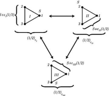
FIG. 23. Three ways of coupling the three spins S on a triangle into a total spin 1 / 2 state. Each construction is related to the two others by the 3j symbols(see text).
ization(CORE) method—in the context of low-dimensional quantum magnetism. This method consists of two steps:(i) building an effective Hamiltonian acting on the low-energy degrees of freedom of some elementary block; and(ii) study-ing this new model numerically on finite-size clusters, usstudy-ing a standard exact diagonalization or similar approach.
Like in other real-space renormalization techniques the effective model usually contains longer range interactions. The numerical CORE procedure will be most efficient pro-vided the effective interactions decay sufficiently fast. We discussed the validity of this assumption in several cases.
For ladder type geometries, we explicitely checked the accuracy of the effective models by increasing the range of the effective interactions until reaching convergence. Both in the perturbative regime and in the isotropic case, our results on a 2-leg ladder and a 3-leg torus are in good agreement with previously established results. This rapid convergence might be due to the small correlation length that exists in these systems which both have a finite spin gap.
In two dimensions, we have used the density matrix as a tool to check whether the restricted basis gives a good enough representation of the exact states. When this is the case, as for the plaquette lattice or the S = 1 / 2 kagomé lattice, the lowest order range-two effective Hamiltonian gives semi-quantitative results, even away from any perturbative regime. For example we can successfully describe the plaquette lat-tice, starting from the decoupled plaquette limit through the quantum phase transition to the Néel ordered state at homo-geneous coupling. Furthermore we can also reproduce many aspects of the exotic low-energy physics of the S = 1 / 2
kagomé lattice.
Therefore within the CORE method, we can have both the advantage of working in a strongly reduced subspace and not being limited to the perturbative regime in certain cases.
We thus believe that the numerical CORE method can be used systematically to explore possible ways of generating low-energy effective Hamiltonians. An important field is for example the doped frustrated magnetic systems, where it is not easy to decide which states are important in a low-energy description, and therefore the density matrix might be a help-ful tool.
APPENDIX A: DENSITY MATRIX
In this appendix we introduce the density matrix of a ba-sic building block in a larger cluster of the fully interacting problem as a diagnostic tool to validate or invalidate a par-ticular choice of retained states on the basic building block in the CORE approach.
In previous applications of the CORE method, the choice of the states kept relied mostly on the spectrum of an isolated building block. While this usually gives reasonable results it is not a clear a priori where to place the cut-off in the spec-trum.
The density matrix of a “system block” embedded in a larger “super block” forms a key concept in the density ma-trix renormalization group (DMRG) algorithm invented by White in 1992 (Ref. 34) and is at the heart of its success. Based on this and related ideas35 we propose to monitor the
density matrix of the basic building block embedded in a larger cluster and to retain these states exhausting a large fraction of the density matrix weight.
Consider now a subsystemA embedded in a larger
sys-temB. Suppose that the overall system B is in state 兩⌿典 (e.g.,
the ground state). We write the wave function as 兩⌿典 =
兺
a,b
a,b兩a典丢兩b典, 共A1兲
where the sum index a runs over all states inA and index b over all states in B\A. The density matrix A of the sub-systemA is then defined as
a,a⬘ A =
兺
b a,ba⬘,b * . 共A2兲The eigenvalues of A denote the probability of finding a certain state a inA, given the overall system in state 兩⌿典.
Practically we calculate the ground state of the fully in-teracting system on a medium size cluster by exact diagonal-ization, and then obtain the density matrix of a basic building block, e.g., a four site plaquette. The density matrix of a building block is a rather local object, so we expect that results on intermediate size clusters are already accurate on the percent level. The density matrix spectra shown in Figs. 8 and 13 have been obtained in this way. In the models con-sidered, a density matrix weight of the retained states of at least 90% yielded reasonable results within a range-two CORE approximation. It is possible to allow for a lower overall weight, at the expense of increasing the range of the CORE interactions.
APPENDIX B: OBSERVABLES IN THE NUMERICAL CORE METHOD
The calculation of observables beyond simple energy re-lated quantities is not straightforward within the CORE method, as the observables need to be renormalized like the Hamiltonian in the first place.3,6
A somewhat simpler approach for measurements of sym-metry breaking order parameters consists in adding a small symmetry breaking field to the Hamiltonian (for a review, see Ref. 30).
Let us denoteOˆ the extensive symmetry breaking opera-tor, such that the order parameter is related to its GS average value m = 1 / N具0兩Oˆ兩0典. The occurrence of a symmetry
bro-ken phase can be detected by adding this operator to the Hamiltonian:
H共␦兲 = H −␦Oˆ. 共B1兲 Since on a finite-size lattice the order parameter vanishes by symmetry for ␦= 0, the ground-state energy per site varies quadratically for small␦
e共␦兲 ⯝ e0− 1 20␦2,
where0 is termed the corresponding generalized
suscepti-bility. In that way the second derivative of the energy with respect to ␦ at ␦= 0 offers one possibility to detect a finite
observe an approximate crossing of the curves if there is a finite order parameter and no crossing in the absence of the order parameter.
Moreover, the derivative of m共␦兲 gives the susceptibility which should diverge at least as the volume squared N2in an ordered phase.30
APPENDIX C: GAUGE INVARIANCE ON HALF-INTEGER SPINS KAGOMÉ LIKE SYSTEMS
In this appendix, we discuss half-integer spin Hamilto-nians with triangles as the unit cell. The ground state mani-fold of each unit cell is generated by the four degenerate lowest states that can be built out of 3 half-integer S spins, namely the four Stot= 1 / 2 states. The idea of selecting these
states as a starting point to describe the whole system low energy properties was originally introduced by Subrahman-yam for S = 1 / 2 (Ref. 25) on the kagomé lattice and later used by Mila.23More recently it was reintroduced by Raghu
et al.26for arbitrary half-integer S in the context of a chain of triangles. All these approaches are pertubative and state that the triangle couplings J is much larger than the intertriangle one J
⬘
.Here we would like to discuss some general properties of any effective Hamiltonian that can be derived either by per-turbative methods or more sophisticated ones such as CORE. In particular, we would like to point out that a gauge invari-ance appears as a direct consequence of the state selection.
To be more specific, let us label 1, 2, 3 the sites of the triangle(see Fig. 21). In order to build a total spin 1/2 out of the three S, spins 2 and 3 couple into a S +共1/2兲 with = ± 1. The coupling with the remaining site 1 produces a spin 1/2 with chirality= ±1. Note that this definition of chirality is equivalent to Eqs.(4) for spin S=1/2 up to a global uni-tary transform which is just a redefinition of the chirality quantification axis.
In the following, the four selected spin-chirality states on a triangle i will be denoted as兩兩i,i典典. These states are the
eigenstates of the z components of spin and chirality (both are spin 1/2 like operators) with z兩兩i,i典典
=共i/ 2兲兩兩i,i典典 andz兩兩i,i典典=i兩兩i,i典典.
Let us now turn to the two-triangle problem. As it can be seen in Fig. 22, the Hamiltonian is invariant under reflections with respect to the共xx
⬘
兲 axis. Moreover, the reflection can be taken independently on each triangle. As a consequence, both chiralities (iz and jz) are conserved by the effective Hamiltonian and the part is of the form 1 + a共iz+zj兲 + bizjz. For any fixed value of 共i,j兲, the total spin of thesystem is conserved and thus the spin part is SU共2兲 invariant.
the particular choice we made for labeling the sites of the triangle(see Fig. 22): site 1 of triangle t1couples to site 1 of
triangle t2. Although this gauge was convenient for the
cal-culation, in general this choice cannot be made simulta-neously on all couples of triangles of the lattice. So, it is essential to derive the form of the Hamiltonian in a generic situation where site i = 1 , 2 , 3 of triangle t1 couples to site j
= 1 , 2 , 3 of triangle t2.
The unitary transformations involved in the redefinition of the coupling sequence (see Fig. 23) are covered by the 3j symbols of elementary quantum mechanics. The problem of 3 half-integer spins S coupled into a total spin 1/2 occurs to be particularly simple and independent of S. The form of the general effective Hamiltonian then reads:
Hij
a,b共␣兲 = 共
i·j+ c共␣兲兲关1 + a共␣兲共i·ea+j· eb兲
+ b共␣兲共i· ea兲共j· eb兲兴,
where ea, a = 1 , 2 , 3 are three coplanar normalized vectors in a 120ⴰ configuration [for example, e1=共0,1兲, e2=共−
冑
3 / 2 ,−1 / 2兲, and e3=共
冑
3 / 2 , −1 / 2兲 in the x-z plane] and a, b arethe labels of the original spins coupling triangles tiand tj. B. The kagomé lattice
In the particular geometry of the kagomé lattice[see Fig. 7(b)], each triangular unit cell is coupled to six other trian-gular cells, each corner being coupled twice. As a conse-quence, for each cell the contribution involving only i· e␣ factorizes into 2i·共e1+ e2+ e3兲=0. The corresponding terms
are then not relevant in the Hamiltonian and thus we denote the most general two-triangle Hamiltonian for the kagomé lattice as H = Na0共␣兲 +
兺
具i,j典关b0共␣兲i · eijj· eij+ a1共␣兲i·j + b1共␣兲i·j共i· eij兲共j· eij兲 + c1共␣兲i·j共i· eij兲 +共j· eij兲兴which is the form used in the text.
ACKNOWLEDGMENTS
We thank F. Alet, A. Auerbach, F. Mila, and D. Poilblanc for fruitful discussions. Furthermore we are grateful to F. Alet for providing us QMC data. We thank M. Körner for his very useful Mathematica spin notebook. A.L. acknowledges support from the Swiss National Fund. We thank IDRIS (Or-say) and the CSCS Manno for allocation of CPU time.
*Electronic address: [email protected]
1C. J. Morningstar and M. Weinstein, Phys. Rev. Lett. 73, 1873 (1994); Phys. Rev. D 54, 4131 (1996).
2M. Weinstein, Phys. Rev. B 63, 174421(2001).
3E. Altman and A. Auerbach, Phys. Rev. B 65, 104508(2002).
4E. Berg, E. Altman, and A. Auerbach, Phys. Rev. Lett. 90,
147204(2003).
5J. Piekarewicz and J. R. Shepard, Phys. Rev. B 56, 5366(1997).
6J. Piekarewicz and J. R. Shepard, Phys. Rev. B 57, 10 260
(1998).
7S. Capponi and D. Poilblanc, Phys. Rev. B 66, 180503(R) (2002). 8J.-P. Malrieu and N. Guihéry, Phys. Rev. B 63, 085110(2001). 9E. Dagotto, and T. M. Rice, Science 271, 618(1996), and
refer-ences therein.
10T. Barnes, E. Dagotto, J. Riera, and E. S. Swanson, Phys. Rev. B 47, 3196(1993); S. R. White, R. M. Noack, and D. J. Scalapino,
Phys. Rev. Lett. 73, 886(1994); B. Frischmuth, B. Ammon, and M. Troyer, Phys. Rev. B 54, R3714(1996).
11M. Greven, R. J. Birgeneau, and U.-J. Wiese, Phys. Rev. Lett. 77,
1865(1996).
12K. Kawano and M. Takahashi, J. Phys. Soc. Jpn. 66, 4001(1997). 13D. C. Cabra, A. Honecker, and P. Pujol, Phys. Rev. B 58, 6241
(1998).
14Proceedings of the 31st Rencontres de Moriond, edited by T.
Martin, G. Montambaux, and J. Trân Thanh Vân(Editions Fron-tières, Gif-sur-Yvette, France, 1996) (cond-mat/9605075).
15E. Lieb, T. Schultz, and D. Mattis, Ann. Phys.(N.Y.) 16, 407 (1961); I. Affleck, Phys. Rev. B 37, 5186 (1988).
16A. Koga, S. Kumada, and N. Kawakami, J. Phys. Soc. Jpn. 68,
642(1999).
17A. Koga, S. Kumada, and N. Kawakami, J. Phys. Soc. Jpn. 68,
2373(1999).
18A. Läuchli, S. Wessel, and M. Sigrist, Phys. Rev. B 66, 014401 (2002).
19A. Voigt, Comput. Phys. Commun. 146, 125(2002).
20P. W. Leung and V. Elser, Phys. Rev. B 47, 5459(1993). 21P. Lecheminant, B. Bernu, C. Lhuillier, L. Pierre, and P.
Sindzin-gre, Phys. Rev. B 56, 2521(1997).
22C. Waldtmann, H.-U. Everts, B. Bernu, C. Lhuillier, P.
Sindzin-gre, P. Lecheminant and L. Pierre, Eur. Phys. J. B 2, 501(1998).
23F. Mila, Phys. Rev. Lett. 81, 2356,(1998).
24M. Mambrini and F. Mila, Eur. Phys. J. B 17, 651(2000). 25V. Subrahmanyam, Phys. Rev. B 52, 1133(1995).
26C. Raghu, I. Rudra, S. Ramasesha, and D. Sen, Phys. Rev. B 62,
9484(2000).
27B. Bernu, C. Lhuillier, and L. Pierre, Phys. Rev. Lett. 69, 2590 (1992).
28P. Sindzingre, C. Lhuillier, and J. B. Fouet, Int. J. Mod. Phys. B 17 5031(2003) (cond-mat/0110283).
29M. Calandra and S. Sorella, Phys. Rev. B 61, R11 894(2000). 30L. Capriotti, Int. J. Mod. Phys. B 15, 1799(2001).
31L. Limot, P. Mendels, G. Collin, C. Mondelli, B. Ouladdiaf, H.
Mutka, N. Blanchard, and M. Mekata, Phys. Rev. B 65, 144447
(2002), and references therein.
32R. Budnik and A. Auerbach(unpublished); R. Budnik, M.Sc.
the-sis, Technion, Haifa.
33S. Dommange, A. Läuchli, J.-B. Fouet, B. Normand, and F. Mila (unpublished).
34S. R. White, Phys. Rev. Lett. 69, 2863(1992).
35C. Zhang, E. Jeckelmann, and S. R. White, Phys. Rev. Lett. 80,
![FIG. 3. (Color online) CORE coefficients [see Eq. (6)] for two](https://thumb-eu.123doks.com/thumbv2/123doknet/2354238.37105/5.918.476.836.82.368/fig-color-online-core-coefficients-eq.webp)