Regionalized Aquatic Ecotoxicity Characterization Factor for Zinc Soil Emissions Accounting for Speciation and for the Transfer Though Groundwater

(1)

UNIVERSITÉ DE MONTRÉAL

REGIONALIZED AQUATIC ECOTOXICITY CHARACTERIZATION FACTOR FOR ZINC SOIL EMISSIONS ACCOUNTING FOR SPECIATION AND FOR THE TRANSFER

THOUGH GROUNDWATER

RIFAT ARA KARIM

DÉPARTEMENT DE GÉNIE CHIMIQUE ÉCOLE POLYTECHNIQUE DE MONTRÉAL

MÉMOIRE PRÉSENTÉ EN VUE DE L’OBTENTION DU DIPLÔME DE MAÎTRISE ÈS SCIENCES APPLIQUÉES

(GÉNIE CHIMIQUE) AOÛT 2018

(2)

UNIVERSITÉ DE MONTRÉAL

ÉCOLE POLYTECHNIQUE DE MONTRÉAL

Ce mémoire intitulé :

REGIONALIZED AQUATIC ECOTOXICITY CHARACTERIZATION FACTOR FOR ZINC SOIL EMISSIONS ACCOUNTING FOR SPECIATION AND FOR THE TRANSFER

THOUGH GROUNDWATER

presenté par : KARIM Rifat Ara

en vue de l’obtention du diplôme de : Maîtrise ès Sciences Appliquées a été dûment accepté par le jury d’examen constitué de :

M. SAMSON Réjean, Ph. D., président

Mme DESCHÊNES Louise, Ph. D, membre et directrice de recherche Mme BULLE Cécile, Ph. D., membre et codirectrice de recherche Mme PLOUFFE Geneviève, Ph. D., membre

(3)

DEDICATION

(4)

ACKNOWLEDGEMENTS

First of all, I would like to thank my proffessors Louise and Cecile for their guidance, support, advice and specially for their patience. You both were warm, welcoming, considerate and I am very fortunate to have both of you as my supervisors. Your insight, attention to detail and encouragement inspired me to continue working on this project and it was my pleasure to work with such incredibly talented women like you.

Many thanks to Geneviève for your patience and integrity. It was you who made it all easy when I was drowing with all sorts of information in the beginning of my project. Many times, I have asked you millions of questions, but you have always managed to answer them. This project would not be a successful one if you were not there for me. Thank you.

I would also like to thank my friends in CIRAIG, pecially Marieke, Lycia, Hassana, Gael, Vincent, Viet for their help in explaining and pointing out many critical aspects of my work during the research.

Thank you Shamsunnahar, Sabreena, Farhana, Nusrat, Thejashree, Sandeep for your friendship. All of you guys were blessings in my life.

Thanks a lot to my kids, Istvan and Ariadne for bringing countless happy moments in our lives. Thank you for being so patient with me even though I was not present in your lives all the time. Thanks to my parents who have always encouraged me in everything I have tried to accomplish, even from thousands of miles away.

Thank you, my dear husband, for keeping up with me and helping me following & fulfilling my dreams in every step of the way.

(5)

RÉSUMÉ

L'analyse du cycle de vie (ACV) est une évaluation des impacts environnementaux d'un produit, d'un processus ou d'un service tout au long de son cycle de vie. Cette évaluation est faite pour une fonction spécifique d'un produit ou d’un processus (par exemple: la fonction de séchage des mains pour un sèche-mains ou de fournir un service de nettoyage pour une entreprise de nettoyage). Le cycle de vie d'un produit peut inclure l'extraction de matières premières, l'acquisition d'énergie, sa production et sa fabrication, son utilisation, sa réutilisation, son recyclage et son élimination finale (fin de vie). Toutes ces étapes du cycle de vie d'un produit contribuent à la production des déchets, des émissions et les consommations des ressources. Ces échanges environnementaux contribuent aux impacts tels que le changement climatique, l'appauvrissement de l'ozone stratosphérique, la formation de photooxydants (smog), l'eutrophisation, l'acidification, le stress toxicologique sur la santé humaine et les écosystèmes, l'épuisement des ressources et la pollution sonore. L'ACV permet de voir où un produit ou un service peut être amélioré ou de fabriquer de meilleurs produits. L'évaluation des impacts environnementaux de cycle de vie est la troisième phase d'ACV dans laquelle le flux de matériaux associés au produit (ou processus) est traduit en consommations de ressources et impacts potentiels sur l'environnement. L'objectif de la phase d'analyse d'impact est donc d'interpréter les inventaires des émissions du cycle de vie et de la consommation des ressources en termes d'indicateurs et d'évaluer l'impact sur les entités que l'on veut protéger. USEtox est un modèle consensuel d'évaluation de l'impact du cycle de vie (ACVI) développé dans le cadre de l'Initiative du cycle de vie du PNUE-SETAC (UN environment programme- Society for environmental toxicology & chemistry). Le développement de ce modèle était une tentative de réduire la variabilité des différents résultats obtenus en utilisant différents modèles d'ACV. Le modèle nous permet de calculer les FC (c'est-à-dire la quantité d'impact environnemental par quantité de substance émise, facterus de caractérisation) pour la toxicité humaine et l'écotoxicité, qui est un produit du facteur d'effet (FE) et du facteur du devenir (FF). L'écotoxicité des métaux est considérée comme mal modélisée par USEtox car la spéciation des métaux n'est pas incluse dans le cadre de calcul.

Lors du consensus de Clearwater, la nécessité de tenir compte de la spéciation des métaux a été identifiée comme l'une des principales priorités par un groupe d'experts pour améliorer l'évaluation de l'impact écotoxicologique des métaux dans l’ACV. Le facteur de biodisponibilité (BF) est inclus

(6)

dans la définition de CF (CF = EF. BF.FF) qui est le rapport de la concentration de métal ‘true’ solution (ions libres et paires d'ions) sur la concentration ‘total’ de métal. Pour être cohérent avec l'inclusion du facteur de biodisponibilité dans les FC, il a également été recommandé d'inclure la spéciation lors du calcul du facteur d'effet (FE). Actuellement, les chercheurs utilisent le ‘Free Ion Activity Model (FIAM)’ (FIAM) et le ‘Biotic Ligand Model’ (BLM) pour prédire l'effet de la concentration de métal dans le milieu aquatique, compte tenu de la spéciation. Le BLM utilise une approche mécaniste basée sur l'hypothèse que l'interaction métal-ligand biotique peut être représentée comme n'importe quelle autre réaction chimique d'une espèce métallique avec un ligand organique ou inorganique.

Dans la version actuelle de USEtox, le compartiment ‘Soil’ est considéré comme un ‘sink’ pour les substances: le sort de la fraction de contaminant qui atteint le compartiment des eaux souterraines par le sol ‘disappears’ et n'est jamais transféré dans les eaux de surface. Cela peut être une hypothèse appropriée pour la plupart des produits chimiques organiques, ce qui peuvent être dégradés avant la résurgence des eaux souterraines que l'écoulement des eaux souterraines est lent, mais cette hypothèse peut représenter un biais important pour les métaux, qui ne sont pas biodégradables et peuvent voyager du sol dans les eaux souterraines par les couches de sol plus profondes, et finalement à l'eau douce. Le destin du métal peut donc ne pas être correctement traité dans USEtox.

La plupart des aquifères et des nappes phréatiques sont interconnectés avec les masses d'eau douce et les mouvements d'eau entre les eaux souterraines et les eaux de surface constituent une voie majeure de transfert de substances chimiques entre les systèmes terrestres et aquatiques. En ne tenant pas compte du sort des métaux dans les eaux souterraines, le sort des métaux dans le sol est surestimé (qui apparaît comme le dernier compartiment où la majeure partie du métal rejeté dans le sol «disparaît») et le devenir du métal dans l'eau de surface est sous-estimée (car les métaux atteignant les eaux souterraines n'atteignent jamais potentiellement l'eau de surface dans le modèle).

Après les précipitations, une fraction de l'eau de pluie s'infiltre à travers la surface terrestre et se déplace verticalement vers le bas jusqu'à la nappe phréatique. L'eau souterraine se déplace alors lentement à la fois verticalement et latéralement avec un écoulement tri-dimensionnel qui se déplace le long des trajets d'écoulement de longueurs variables allant des zones de recharge aux

(7)

zones de décharge. Un bassin versant (analogue à un «bassin hydrographique» ou «bassin versant») est défini comme une zone de drainage des eaux de pluie jusqu'à ce qu'elle atteigne le même plan d'eau (une rivière, un lac ou l'océan). Les limites des bassins versants sont basées sur la topographie du sol et les cours d'eau. Le bassin versant peut être considéré comme le niveau de résolution géographique auquel toute goutte de pluie qui tombe sur le sol atteindra le même plan d'eau (et tous les contaminants transportés par ce courant d'eau).

L'estimation du comportement des eaux souterraines nécessite une modélisation de l'interaction entre tous les processus importants du cycle hydrologique, tels que la couverture terrestre, le profil du sol, l'infiltration, le ruissellement, l'évapotranspiration, la fonte des neiges et les variations des eaux souterraines. La description quantitative des processus hydrologiques peut devenir très compliquée en raison de l'incertitude et de la complexité élevées des paramètres physiques sous-jacents. Cependant, dans le ACVI, l'évaluation des l'impacts toxiques est généralement réalisée en utilisant des modèles d'état d'équilibre simplifiés tels que USEtox. L'un des principes importants de USEtox est d'être parcimonieux et d'inclure uniquement les mécanismes environnementaux les plus pertinents. Par conséquent, l'intégration du transfert des contaminants dans les eaux souterraines dans ACVI devrait également être effectuée avec parcimonie dans une version adaptée de USEtox, permettant seulement de quantifier la masse de contaminant transférée du sol à l'eau de surface à l'état stationnaire, sans détails sur la voie du contaminant dans le compartiment de sous-sol/ des eaux souterraines et sur la cinétique des processus hydrologiques. L'objectif de la présente étude est de développer une telle version de USEtox pour calculer les facteurs de caractérisation écotoxicologiques des eaux souterraines (CF) pour un émission dans les sols, en tenant compte de la spéciation dans tous les compartiments environnementaux (sol, sous-sol et eau souterraine, eau douce) et de l'appliquer au cas du zinc.

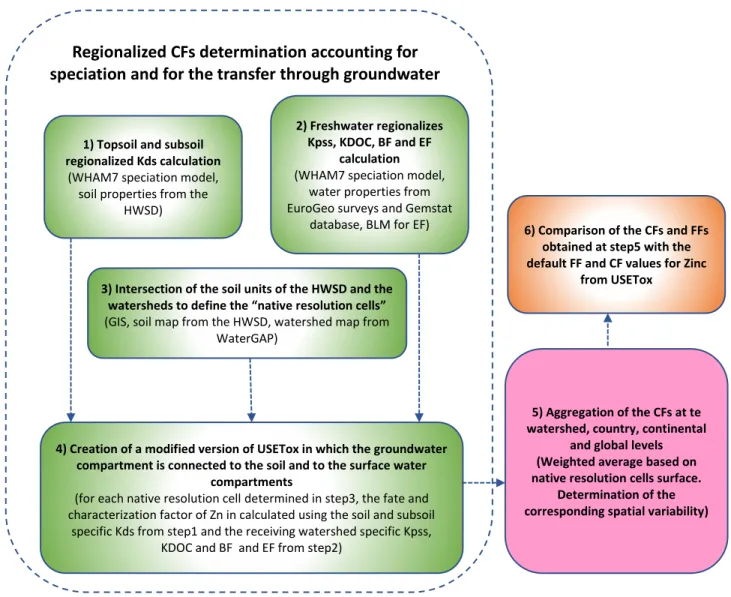
Pour le calcul du facteur de devenir (FF) et du facteur de caractérisation (FC) en considérant l'émission de Zn dans le sol, les calculs sont effectués en plusieurs étapes: d'abord, les coefficients de partage sol / eau du sol et du sous-sol sont calculés en utilisant le logiciel de spéciation WHAM7 pour toutes les différentes unités de sol et de sous-sol de la base de données mondiale harmonisée sur les sols (HWSD). Deuxièmement, des calculs de spéciation sont également effectués dans le compartiment d'eau douce, sur la base des données disponibles sur les propriétés de l'eau douce partout dans le monde et en utilisant le modèle de spéciation WHAM. Troisièmement, un système d'information géographique est utilisé pour recouper les unités de sol et les bassins versants afin

(8)

d'obtenir des cellules géographiques (cellules de résolution native). Dans chacune de ces cellules, on considère que Zn a les coefficients de partage sol-eau pour les compartiment des sol et sous-sol correspondant à sa spéciation dans cettes compartiments et aussi que Zn a des coefficients de partage solide-eau suspendu et octanol-eau correspondant de sa spéciation dans l’eau pour cette bassin versant specifique. Quatrièmement, USETox est modifié en reliant a) le sol au sous-sol et au compartiment des eaux souterraines et b) le sous-sol et le compartiment des eaux souterraines au compartiment d'eau douce. Les facteurs de devenir du sol à l'eau (FFsw) pour chaque cellule de résolution naturelle sont calculés en utilisant ces coefficients de partage du sol, du sous-sol et du bassin versant dans la version modifiée d'USETox. Ces FFsw s spécifiques aux cellules de résolution native sont multipliées par des facteurs de biodisponibilité spécifiques (BF) et des facteurs d'effets (EF) pour générer des facteurs de caractérisation du sol (CFsw) pour toutes les cellules de résolution native disponibles dans le monde entier. Cinquièmement, les résultats obtenus à l'échelle de la résolution native sont agrégés à différentes échelles de régionalisation plus opérationnelles: bassin versant, pays, continent et niveau global, avec la détermination de la variabilité spatiale correspondante. Enfin, les résultats sont comparés aux valeurs par défaut calculées par USETox.

Les facteurs de caractérisation régionaux de l'écotoxicité des eaux douces pour le zinc émis dans le sol ont une variabilité spatiale globale sur 3 ordres de grandeur et la valeur globale moyenne pondérée est dans le même ordre de grandeur que la valeur USETox par défaut (1,42 fois inférieure). La variabilité spatiale des facteurs de sort du Zn du sol à l'eau (FFsw) et des facteurs de caractérisation du Zn (CFsw) dans chaque bassin versant est quantifiée. Les résultats sont illustrés sur une carte du monde pour toutes les cellules de résolution native pour lesquelles des données sont disponibles. À l'exception de l'Europe, tous les FFsw et CFsw régionaux et continentaux ont varié de plus de 2 ordres de grandeur. Pour l'Europe, une variabilité spatiale de 3 ordres de grandeur est observée parce que (1) la variabilité spatiale de la spéciation régionale dans le sol est plus grande (2) des données régionalisées pour l'eau douce sont disponibles pour de nombreux sites à travers le continent ainsi que à une plus grande variabilité spatiale de la spéciation dans l'eau.

(9)

L'une des principales limites de l'étude est la faible disponibilité des données régionalisées sur l'eau douce nécessaires à l'exécution du modèle de spéciation. Avec les données actuelles disponibles, la variabilité spatiale des CFs pour Zn à l'échelle continentale est proche de l'incertitude des CFs de l'USEtox (deux ordres de grandeur), ce qui signifie que l'utilisation d'un CF continentale semble un compromis raisonnable entre une collecte de données trop intensive et une évaluation d'impact imprécise.

(10)

ABSTRACT

Life cycle assessment (LCA) is the assessment of environmental impacts of a product, process or service across its entire life cycle. This assessment is done based on a particular function of the product or process (for example: the function of drying hands for a hand dryer or providing cleaning service for a cleaning company). A product’s life cycle can include the extraction of raw materials, energy acquisition, its production and manufacturing, use, reuse, recycling and ultimate disposal. All these stages in a product’s life cycle result in the generation of wastes, emissions, and the consumption of resources. These environmental exchanges contribute to impacts such as, climate change, stratospheric ozone depletion, photooxidant formation (smog), eutrophication, acidification, toxicological stress on human health and ecosystems, depletion of resources, and noise pollution among others. LCA allows us to see where a product or service can be improved or manufacturing of new better products. Life cycle impact asssesment is the third phase of LCA in which the flow of materials associated with the product (or process) is translated into consumptions of resources and potential impacts to the environment. The purpose of the impact assessment phase is thus to interpret the life cycle emissions and resource consumption inventory in terms of indicators and to evaluate the impact on the entities that we want to protect.

USEtox is a consensual life cycle impact assessment (LCIA) model developed within the UNEP-SETAC Life Cycle Initiative. The development of this model was an attempt to reduce the variability of different results obtained from using different LCA models. The model allows us to calculate CFs (ie the quantity of environmental impact per quantity of substance emitted) for human toxicity and ecotoxicity which is a product of Effect Factor (EF) and Fate factor (FF). Metal ecotoxicity is considered as poorly modeled by USEtox as the metal speciation is not included within the calculation framework.

During the Clearwater consensus, the need to account for metal speciation has been identified as one of the key priorities by a group of experts to improve the ecotoxicological impact assessment of metals in LCA. The bioavailability factor (BF) is included within the definition of CF (CF= FF.BF.EF) which is the ratio of the true solution (free ions and ion pairs) metal concentration over total metal concentration. To be consistent with the inclusion of bioavailability factor in the CF, it was also recommended to include speciation while calculation the Effect Factor (EF). Currently, researchers use Free Ion Activity Model (FIAM) and Biotic Ligand Model (BLM) to predict the

(11)

effect concentration of metal in aquatic environment accounting for the speciation. BLM uses a mechanistic approach that is based on the hypothesis that the metal–biotic ligand interaction can be represented like any other chemical reaction of a metal species with an organic/inorganic ligand. In the current version of USEtox, the soil compartment is considered as a sink for the substances: the fate of the fraction of contaminant that reaches the groundwater compartment through soil, “disappears” and is never transferred to the surface water. This may be an appropriate assumption for most organic chemicals, which may degrade before the resurgence of groundwater as the groundwater flow is slow. However, this assumption may represent an important bias for the metals, which are not biodegradable and may travel from soil to groundwater through the deeper soil layers, and ultimately to freshwater. The metal fate may therefore not be properly addressed within USEtox.

Most of the aquifers and groundwater table are interconnected with the freshwater bodies and water movement between groundwater and surface water is a major pathway for chemical transfer between terrestrial and aquatic systems. By not considering the fate of metal through groundwater, the fate of metals to the soil is overestimated (which appears as the ultimate compartment where most of the metal emitted to soil “disappears” from the system when transferred to groundwater) and the fate of metal to the surface water is underestimated (as metals reaching the groundwater never potentially reaches surface water in the model).

After precipitations, a fraction of the rainwater infiltrates through the land surface and moves vertically downward to the water table. The ground water then moves slowly both vertically and laterally with a three-dimensional flow, which moves along flow paths of varying lengths from areas of recharge to areas of discharge. A watershed (analogous with ‘drainage basin’ or ‘catchment area’) is defined as an area of land that drains down the precipitation until it reaches the same water body (a river, a lake or the ocean). Watershed boundaries are based on soil topography, watercourse and stream locations. The watershed can be considered as the geographical resolution level at which any raindrop that falls on the soil will reach the same water body (and so do all the contaminants transported by this water flow).

Estimation of the groundwater behaviour requires modelling of the interaction between all of the important processes in the hydrologic cycle, such as land cover, soil profile, infiltration, surface runoff, evapotranspiration, snowmelt and variations in groundwater. The quantitative description

(12)

of the hydrologic processes may become very complicated due to the high uncertainty and complexity in the underlying physical parameters. However, in LCIA, toxic impact assessment is generally conducted using simplified steady-state models such as USEtox. One of the important principles of USEtox is to be parsimonious and to include only the most relevant environmental mechanisms. Hence, the integration of the transfer of contaminant through groundwater in LCIA should also be done parsimoniously in an adapted version of USEtox, only allowing to quantify the mass of contaminant transferred from soil to surface water at steady state through groundwater, without details about the pathway of the contaminant in the subsoil / groundwater compartment and about the hydrologic processes kinetics. The objective of the present study is to develop such a version of USEtox to calculate regionalized freshwater ecotoxicity characterization factors (CF) for metal soil emissions accounting for the missing link from topsoil to freshwater though groundwater and considering speciation in all the environmental compartments (soil, subsoil & groundwater, freshwater) and to apply it to the case of Zinc.

For the soil to water fate factor (FF) and characterization factor (CF) calculation considering Zn emission to soil, calculations are performed in several steps: first, the soil/water partitioning coefficients (Kd) for Zn in soil and in subsoil is determined using the WHAM7 speciation software for all the different soil and subsoil units from the harmonized world soil database (HWSD). Second, speciation calculations are also performed in the freshwater compartment, based on available data about freshwater properties all over the world and using the WHAM speciation model. Third, a geographic information system is used to intersect soil units and watersheds to obtain some geographical cells (native resolution cells). In each of those cells, it is considered that Zn has soil-water partition coefficients in the soil and subsoil compartments corresponding to its speciation in those compartments and that Zn also has suspended solid-water and octanol-water partition coefficients in the surface water compartment corresponding to Zn speciation in water within that specific watershed. Fourth, USETox is modified by linking a) the soil to the subsoil & groundwater compartment and b) the subsoil & groundwater compartment to the freshwater compartment. Fate factors from soil to water (FFsw) for each native resolution cell are calculated using these soil, subsoil and watershed level partition coefficients in the modified version of USETox. These native resolution cell specific FFsws are multiplied with watershed specific bioavailability factors (BFs) and effect factors (EFs) to generate soil to water characterization factors (CFsw) for all the native resolution cells for which data is available around the globe. Fifth,

(13)

the results obtained at the native resolution scale are aggregated at different more operational regionalization scales: watershed, country, continent and global level, with the corresponding spatial variability determination. Lastly, the results are compared to the default values calculated by USETox.

Regionalized freshwater ecotoxicity characterization factors for zinc emitted to soil have a global spatial variability over 3 orders of magnitude and the weighted average global value is in the same order of magnitude than the default USETox value (1.42 times lower). The spatial variability of the Zn fate factors from soil to water (FFsw) and of the Zn characterization factors (CFsw) within each watershed is quantified. The results are illustrated on a world map for all the native resolution cells for which data is available. With the exception of Europe, all the regional and continental FFsw and CFsw varied over 2 orders magnitude. For Europe, a spatial variability of 3 orders of magnitude is observed because (1) the spatial variability of regional speciation in soil is larger (2) spatial data for freshwater is available for many locations across the continent thereby leading to a higher spatial variability of the speciation in water.

One of the main limits of the study is the low availability of regionalized freshwater data needed to run the speciation model. With the current available data, the spatial variability of Zn CFs at continental scale is close to the uncertainty of USEtox CFs (two orders of magnitude), meaning that using a continental level CF seems a reasonable compromise between a too intensive data collection and a too imprecise impact assessment.

(14)

LIST OF TABLES

Table 2-1 Available CFs of metals from different LCIA models ... 11

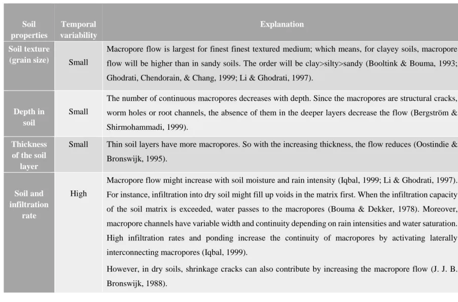
Table 2-2 Dependency of macropore flow on soil properties: adopted from (Hellweg, Fischer et al. 2005) ... 26

Table 2-3 Fraction of macropore flow compared to the total flow in silty and clayey soils adopted from: (Hellweg, Fischer et al. 2005) ... 27

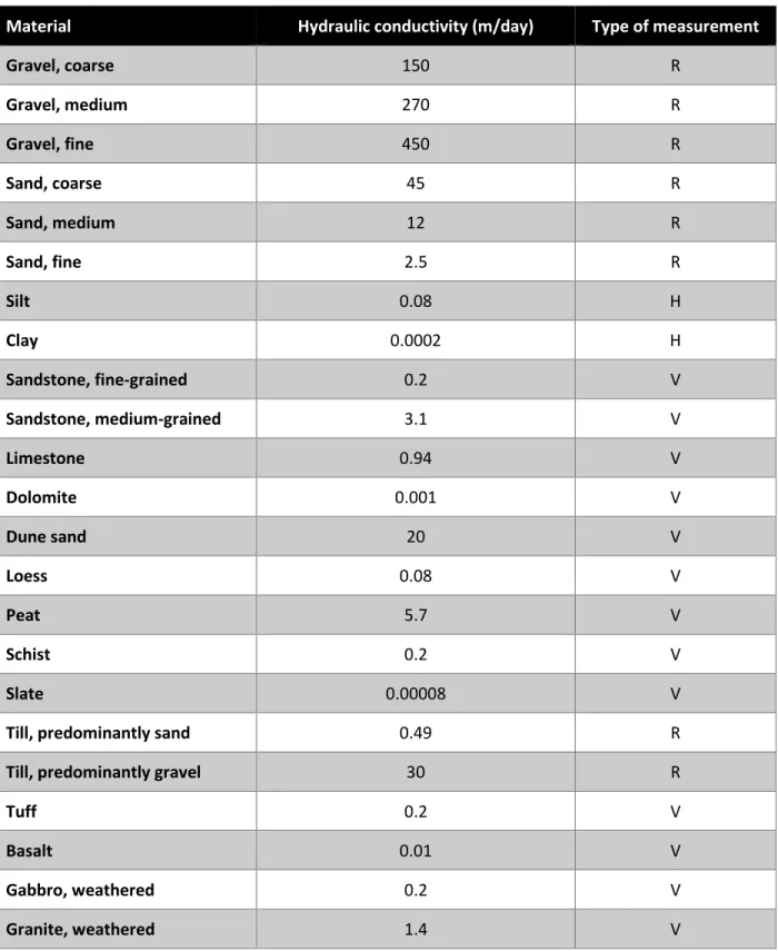
Table 2-4 Representative values of hydraulic conductivity. Source: Morris and Johnson (1967), Todd and Mays (2005) ... 31

Table A5 Properties of the Subsoil & groundwater compartment ... 86

Table A6 Continental SubSoil & groundwater volume from Margat (2008) ... 87

Table A7 Region specific data choices for fate and characterization calculations. ... 91

Table A8 Aggregated soil to water fate and characterization factors for different regions ... 94

(18)

LIST OF FIGURES

Figure 2-1 Framework (four phases) of LCA study ... 5 Figure 2-2 Impact categories for characterisation modelling at midpoint and endpoint (Areas of Protection) levels (Hauschild, Goedkoop et al. 2009) ... 6 Figure 2-3 Different compartments in the USEtox model (Rosenbaum, Bachmann et al. 2008) . 12 Figure 2-4 The USEtox assessment steps for the calculation of fate (Rosenbaum, Bachmann et al. 2008) ... 13 Figure 4-1 General methodological steps followed for this study ... 48 Figure 4-2 Modification of the fate model in USETox ... 56 Figure 4-3 Violin plot showing the variability of the soil-water partitioning coefficient in top soils (Kd), subsoil & groundwater (Kd) compartments. The violin representing the probability density and the box plots representing the, values with 95% confidence interval, median values and the interquartile ranges. ... 59 Figure 4-4 Plots showing the variability and distribution in a) Bioavailability factors (BF) and b) Effect factors (EF) for all water properties around the world ... 61 Figure 4-5 Variabilities at the native resolution scale regionalized values of (a) the soil to water fate factors (FFsws) and (b) the freshwater ecotoxicity characterization factors (CFsw) for an emission to soil ... 65 Figure 4-6 Soil to water characterization factors (CFsw) for watersheds for different regions of the world ... 66 Figure 4-7 Spread and frequency of the soil to water characterization factors (CFsw) with the aggregated CFsw value and the default USETox value ... 67 Figure A8 Map of USA subdivided into 3 sections and proximity of the Canadian stations from the GEMStatPortal (2017) database justifies the use of those data as proxies for toxicity calculations within the USA ... 93 Figure A9 Topsoil partition coefficient Kd (L/Kg) for all HWSD topsoil Units ... 95 Figure A10 Subsoil partition coefficient Kd (L/Kg) for all HWSD subsoil Units ... 95

(19)

LIST OF SYMBOLS AND ABBREVIATIONS

BF Bioavailablity Factor BLM Biotic Ligand Model CF Characterization Factor DOC Dissolved Oxygen Content

EF Effect Factor

FF Fate Factor

LCA Life Cycle Analysis

LCIA Life Cycle Impact Analysis OM Organic Matter Content

SETAC Society For Environmental Toxicology And Chemistry TBLM Terrestrial Biotic Ligand Model

UNEP United Nations Environmental Program WHAM Windermere Humic Aqueous Model

(20)

LIST OF APPENDICES

APPENDIX A (ELECTRONIC SUPPLEMENTARY MATERIAL-1) ... 86 APPENDIX B (ELECTRONIC SUPPLEMENTARY MATERIAL-2)...……….96 APPENDIX C(ELECTRONIC SUPPLEMENTARY MATERIAL-3)….……….96

(21)

CHAPTER 1 INTRODUCTION

In life-cycle analysis (LCA), metals’ ecotoxicological impacts are always on the higher side. It is partly because of the consideration of the total metal concentration within the calculations. And also, all these models (IMPACTWorld, IMPACT2002, USES-LCA, CalTOX, LUCAS etc.) were initially built for organics later they were developed for metals. One of the many assumptions for the organic material were they are biodegradable and do not undergo speciation which is not true for the metals since they are persistent in nature, keep accumulating every day and can have variable valance states, thereby voiding the use of those models for metal toxicity calculations (Christensen et al., 2007; Haye, Slaveykova, & Payet, 2007; Pizzol, Christensen, Schmidt, & Thomsen, 2011a).

Even if one like to choose from the abovementioned model for metal toxicity calculations, all of the models vary in their scope and modeling principles. The inter-model results variations and uncertainty due to the assumptions are very high. Choosing a single model for specific calculations and making modifications and then adapting for others will introduce erroneous results (Pizzol et al., 2011a; Pizzol, Christensen, Schmidt, & Thomsen, 2011b).

USEtox model is developed as the results of scientific consensus among these model developers: CalTOX, IMPACT 2002, USES-LCA, BETR, EDIP, WATSON and EcoSense. The development of this model was an attempt to reduce the variability of different results from different LCA models. Through this process, the inter model variation was reduced from an initial range of up to 13 orders of magnitude down to no more than two orders of magnitude for any substance (Rosenbaum et al., 2008).

Moreover, integrating metal along with speciation and regionalization within LCA is challenging, given the lack of precise information on LCA emissions, choice of methods speciation calculations and inadequate model assumptions. The study on Zn by Ligthart, Jongbloed, and Tamis (2010) for gutter and downpipes using CML method showed a considerable decrease in the freshwater (25%) and marine aquatic ecotoxicity potential (42%) pointing to the fact that total metal concentration is in fact not a good indicator of metal fate. It also implies that total metal concentration is not responsible for detrimental effects on human health and ecosystems. It was recommended in the Clearwater workshop by Diamond et al. (2010) to include the bioavailability fractor of metal (the ratio of truly solution metal by total metal) which is considered to be the best indicator for toxic

(22)

effects in all fate and effect calculations. It was suggested the use of a geochemical speciation model, in particular the WHAM 6.0 model (Windermere Humic Aqueous Model, then available version) to obtain the bioavailable fraction and the use of archetypes of the same properties to consider the spatial variability of environmental properties (Diamond et al., 2010). Considerable progress have been made after the work done by Gandhi et al. (2010), Gandhi, Huijbregts, et al. (2011) and Gandhi, Diamond, et al. (2011) with Cu, Ni and Zn in case of aquatic ecotoxicity in terrestrial ecosystems in European freshwater. Dong, Gandhi, and Hauschild (2014) had implemented the previous method and extended the toxicity calculations on 14 cationic metals (Al, Ba, Be, Cd, Co, Cr, Cs, Cu, Fe, Mn, Ni, Pb, Sr, Zn). (Diamond et al., 2010; Dong et al., 2014; Gandhi, Diamond, et al., 2011; Gandhi et al., 2010; Gandhi, Huijbregts, et al., 2011). Although WHAM 6 was tested for water, it was first evaluated and validated for soils first by Plouffe, Bulle, and Deschênes (2015). The calculated Zn characterization factors after incorporating the true solution Zn and soluble Zn by Plouffe, Bulle, and Deschênes (2016) are lower than the values calculated using traditional methods. The results point out the importance of considering speciation in heterogenous media like soils. However, it also raises the question that the soluble metal fractions might leach to the deeper soil layers and soil has a finite infiltration capacity.

In reality, the transfer of contaminants in the soil depends on physicochemical properties of the soil and the substance. The infiltration capacity of a soil determines whether and how much of the water can seep into the deeper soil layer. Groundwater represents one portion of the earth’s water circulatory system known as the hydrologic cycle. It constitutes 0.39% of the world’s water but 49% of the world’s freshwater. Water-bearing formations of the earth’s crust act as conduits for transmission and as reservoirs for storage of water. Water enters in these formations from natural recharges such as, precipitation, streamflow, lakes and reservoirs and travels slowly for varying distances until it returns to the surface by action of natural flow, plants or humans (Aral & Taylor, 2011; Bowen, 1979; "Groundwater Hydrology," ; Todd & Mays, 2005).

The objective of this study is to make modifications within USEtox considering the missing link from topsoil to freshwater though groundwater and considering speciation in all the environmental compartments (soil, subsoil & groundwater, freshwater) thereby calculating regionalized soil to freshwater Zn characterization factors (CF). The methodology proposed in this project is as follows. The use to WHAM 7 (latest version) to perform speciation with the regionalized soil properties available over the world from HWSD database (HWSD-database, 2014). After that, the

(23)

soluble Zn fraction from soil will be added with the modified version of the USETox model in which soil, groundwater and surface water system are connected. Soil to water fate and characterization factors will be calculated in native soil resolution. Calculations will also be performed for watershed specific resolution and aggregated fate and characterization factors over continents and regions. The reulsts will be further compared with the USETox default results. The first chapter of this thesis contains literature review followed by research hypothesis, justification of choice, objectives and methodology in Chapter 2. Chapter 3 is the manuscript from the project that has been submitted to the International Journal of LCA. Finally, Chapter 3 discusses the conclusion drawn and overall perspectives from the project.

(24)

CHAPTER 2 LITERATURE REVIEW

This chapter begins with the explanation of Life Cycle Analysis (LCA) and the various steps involved to perform a complete LCA. The challenges with metals in LCA in aquatic and terrestrial ecotoxicology are described and the choice of metal to be studied is justified. State of the art of the current mathematical modelling in LCA and the limitations are discussed toward the end.

2.1 Life Cycle Analysis (LCA)

2.1.1 Definition, Characteristics and Steps of LCA

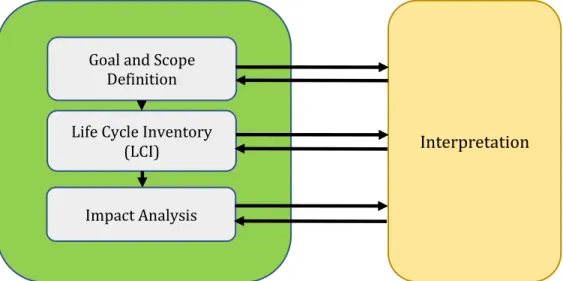
Life cycle assessment is the assessment of environmental impacts of a product, process or service across its entire life cycle. This assessment is done based on a particular function of the product or process (for example: the function of drying hands for a hand dryer or providing cleaning service for a cleaning company). A product’s life cycle can include the extraction of raw materials, energy acquisition, its production and manufacturing, use, reuse, recycling and ultimate disposal. All these stages in a product’s life cycle result in the generation of wastes, emissions, and the consumption of resources. These environmental exchanges contribute to impacts such as, climate change, stratospheric ozone depletion, photooxidant formation (smog), eutrophication, acidification, toxicological stress on human health and ecosystems, depletion of resources, and noise pollution among others. LCA allows us to see where a product or service can be improved or manufacturing of new better products. According to the series of ISO14040 standards and SETAC (Society for Environmental Toxicology And Chemistry) definition, any LCA study should consist of four steps. The study begins with (1) Goal and scope definition, then (2) Life cycle inventory (LCI), (3) Life cycle impact assessment (LCIA) and finally (4) Interpretation (Michael Zwicky Hauschild et al., 2002; Jolliet, Saadé, Crettaz, & Shaked, 2010; Tillman & Baumann, 2004).

The first step deals with the definition and setting the objectives, a description and scope of the study, the type of application of LCA study (to be) performed, target audience, the stakeholders and the functional unit. The frontiers of the system and the reference flows are also defined in this step. Unlike other phases of the LCA, the phase is not very technical, but has a strong participatory dimension (Jolliet et al., 2010).

(25)

The next phase of LCA is to establish an inventory of all incoming and outgoing flows of the system during the stages of the life cycle. If all steps are considered, LCA will be called "cradle to grave" as opposed to LCA "cradle to gate" [at the factory]. In the latter type, the phases of use and end of life are excluded. It is useful for the assessment of the intermediate products which are not intended for the consumer. Inventory data can come from the same manufacturers and suppliers (primary data) or specialized databases (secondary data) such as ecoinvent (Canals et al., 2011; Jolliet et al., 2010).

The impact assessment step assesses the impact on the environment and emissions from extractions which were inventoried in the previous phase. This step sometimes can be broken down into four stages. This stduywill deal with metal contamination in aquatic and terrestrial ecosystem which fall within this very step and is discussed in more detail in section 2.2 (Jolliet et al., 2010).

Interpretation step allows to interpret the results in each of the preceding phases and also to assess uncertainties related with them. The key points and options for improvement of the product studied are well identified. This last phase can (also) be completed by linking it with the environmental aspects and economic or social aspects (Jolliet et al., 2010).

The four phases of LCA are presented in Figure 2-1 (Jolliet et al., 2010).

Figure 2-1 Framework (four phases) of LCA study

Interpretation Goal and Scope

Definition

Impact Analysis Life Cycle Inventory

(26)

2.2 Life cycle impact assessment (LCIA)

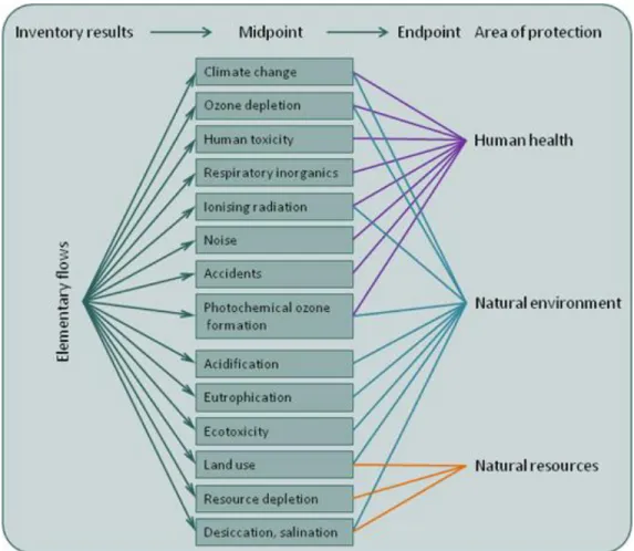
In this third phase of LCA the flow of materials associated with the product (or process) is translated into consumptions of resources and potential impacts to the environment. The purpose of the impact assessment phase is thus to interpret the life cycle emissions and resource consumption inventory in terms of indicators for the Areas of Protection (AoPs), i.e. to evaluate the impact on the entities that we want to protect. The Areas of Protection (presented in Figure 2-2) considered according to ILCD (international Reference on Life Cycle Data System) handbook are: ‘Human Health’, ‘Natural Environment’ and ‘Natural Resources’ (Michael Hauschild et al., 2009a, 2009b).

Figure 2-2 Impact categories for characterisation modelling at midpoint and endpoint (Areas of Protection) levels (Michael Hauschild et al., 2009b)

(27)

According to ISO 14044, Life Cycle Impact Assessment (LCIA) proceeds through four steps : (a)

Classification (mandatory): In this step, the elementary flows from the life cycle inventory are

then assigned to impact categories according to the pollutant’s ability to contribute to different environmental problems. (b) Characterisation (mandatory): The relative contributions of the emissions and resource consumptions to each type of environmental impact are calculated in this step. (c) Normalisation (optional): The characterised impact scores are associated with a common reference, such as the impacts caused by one person during one year in a stated geographic context.

(d) Weighting (optional): The different environmental impact categories and/or Areas of

Protection are ranked according to their relative importance. Weighting is necessary when trade-off situations occur in LCAs, or comparing alternative products (Michael Hauschild et al., 2009b; Tillman & Baumann, 2004).

The path that is followed by any pollutant from its emission to final impact is called impact pathway. In LCIA, impacts on the Areas of Protection are modelled by applying knowledge about the relevant impact pathways or environmental mechanisms (Michael Hauschild et al., 2009a; Jolliet et al., 2010).

Identification and quantification of impacts on human health and ecosystems due to emissions of toxic substances are very important for the development of sustainable products and technologies. Toxicity indicators (characterization factors) for human health effects and ecosystem quality are necessary both for comparative risk assessment and for LCAs applied to chemicals and emission scenarios. However, in practice, there are discrepancies and differences in results from using different models and they often fail to arrive at the same toxicity characterisation score for a substance (Rosenbaum et al., 2008).

Different LCIA methodologies and models have been developed over time: researchers have often updated and renovated their previously developed models and then released new versions (example: EDIP 97 was substituted by the more developed EDIP 2003). In some cases different research teams collaborated in order to reach some consensus and develop new methods based on the best features of the old ones (ReCiPe originated from the two existing methods CML 2001 and Eco-Indicator 99) (Pizzol et al., 2011b).

Generally, the impact from any product or process (on health or ecosystems) emitted in any environmental compartment (air, water, soil) is estimated by multiplying the mass of the

(28)

contaminant emitted by a characterization factor (CF). This characterization factor is obtained by multiplying the fate factor (FF) with an effect factor (EF). FF is the fraction of substance transferred from the compartment of emission to the compartment of reception and its residence time in it (Haye et al., 2007). The effect factor (EF) is the effect of the substance on organisms as per concentration of exposure (Haye et al., 2007).

2.2.1 Fate & impact characterization modeling in LCA

Several characterization methods are currently used in LCA. Some methods as EDIP 97, make a partial evaluation with key physicochemical properties. Others, such USES-LCA and IMPACT 2002+ use multimedia models. These models generally consist of steady state first order differential equations for representing contaminant distribution between different environmental compartments (eg. Air, water, soil, sediment), degradation and advective transport. The major part of fate models were developed for environmental risk analysis of and initially to assess the fate of non-ionic organic compounds. However, some models have been developed directly for comparative methods like LCA (ex. USES-LCA and IMPACT 2002) and some models were applied to metals (eg. EUSES and CalTOX) (Bachmann, 2006; Michael Z Hauschild et al., 2008; Pennington, Margni, Ammann, & Jolliet, 2005).

Some of the LCIA models take into account the spatial variability of some environmental parameters. For example, IMPACT 2002 model has a spatial version where Western Europe is divided into 135 zones. For the terrestrial environment distributed according pools 124 zones and ocean areas (each with 2 compartments and 1 water sediment compartment) and 157 zones for air divided into a grid of 2 by 2.5 degrees for air and oceans Each watershed is considered to be composed of the following compartments: soil compartment, a surface water compartment, a sediment compartment and agricultural vegetation compartment. The model assumes degradation, intermedia transfer and advection and emissions in surface water, ocean, soil and air (Godin, 2004; M. A. Huijbregts et al., 2000; Sebastien Humbert et al., 2009; Toffoletto, Bulle, Godin, Reid, & Deschênes, 2007).

The spatial version of the IMPACT 2002 model then has been adapted to the Canadian geographic context taking into account the differences between the characteristics of Canada and Europe including the population and area (Toffoletto et al., 2007).

(29)

The spatial differentiation in the LUCAS method (LCIA method Used for A Canadian-Specific context) is based on 15 Canadian ecozones and each ecozone has its own characteristics related to climate, soil, fauna, flora and human activities. The development of CF in ecotoxicity in LUCAS is currently done with a version of the IMPACT model 2002 adapted in Canadian context by integrating chemical properties of representative average environmental conditions. The IMPACT 2002 model is also the basis of IMPACT North America model which is a fate and exposure model and takes into account the geographical distribution in North America. The model was tested for benzopyrene, 2,3,7,8-TCDD and mercury (Hg) (Sebastien Humbert et al., 2009; Toffoletto et al., 2007).

The problem of using these abovementioned models with metals are, initially they were developed for organic substances, later they were made applicable to inorganics. The uncertainties due to this adaptation is quite high. Also, the documentation of assumption and calculation for most of the existing LCIA models are not very transparent. Choosing any single model which is not very well documented and then trying to make a modification within itself will pose a big challenge and introduce errors (Pizzol et al., 2011a, 2011b)

It is evident that the models vary in their scope and modeling principles, and hence also in terms of the characterization factors they generate. However, ISO has refrained from standardization of the detailed methodologies in LCA. So, with the scientific consensus of the scientists and with a careful focus on the most influential model elements, the USEtox model was established. (Dreyer, Niemann, & Hauschild, 2003; Michael Z Hauschild, 2005; Michael Z Hauschild et al., 2008; Henderson et al., 2011; Pizzol et al., 2011a, 2011b).

USEtox model is the results of scientific consensus among these model developers: CalTOX, IMPACT 2002, USES-LCA, BETR, EDIP, WATSON and EcoSense. This method performs a systematic analysis of the approaches used in analyzing the impact on the life cycle, supplementing them with a selection of environmental models not currently integrated in LCA methodologies, but with interesting features (Michael Z Hauschild et al., 2008). The development of this model was an attempt to reduce the variability of different results from different LCA models. Through this process, the inter model variation was reduced from an initial range of up to 13 orders of magnitude down to no more than two orders of magnitude for any substance (Rosenbaum et al., 2008).

(30)

The undelying four principles of the model were, that it should be parsimonious (as simple as possible, as complex as necessary), mimetic (not differing from the original models than these differ among themselves), evaluative (providing a repository of knowledge through evaluation against a broad set of existing models) and transparent (well-documented, including the reasoning for model choices). The model was kept simple and only involving the most important inter media mechanisms in order to limit the enormous amount of data requirement, since the scarcity of data is always a concern in LCA (Rosenbaum et al., 2008).

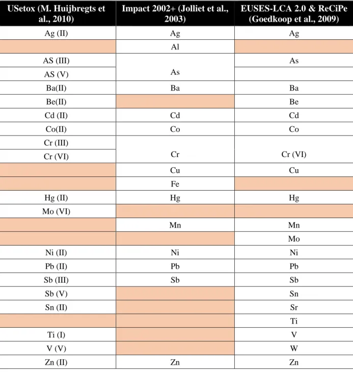
Currently, the models provide characterization factors for non-ionic and nonpolar organic compounds (as they were developed) and CF for around 18 metals although they have very strong uncertainty and were calculated only interim measure until more robust models are established (MichaelZ Hauschild et al., 2013; M. Huijbregts et al., 2010; Rosenbaum et al., 2008).Table 2-1 provides a list of metal whose CFs were generated from USEtox (freshwater ecotoxicity), IMPACT 2002+ (Terrestrial and aquatic ecotoxicity) , EUSES-LCA 2.0 and ReCiPe (freshwater aquatic ecotoxicity, marine ecotoxicity and terrestrial ecotoxicity) models.

(31)

Table 2-1 Available CFs of metals from different LCIA models

USetox (M. Huijbregts et al., 2010)

Impact 2002+ (Jolliet et al., 2003)

EUSES-LCA 2.0 & ReCiPe (Goedkoop et al., 2009) Ag (II) Ag Ag Al AS (III) As As AS (V) Ba(II) Ba Ba Be(II) Be Cd (II) Cd Cd Co(II) Co Co Cr (III) Cr Cr (VI) Cr (VI) Cu Cu Fe Hg (II) Hg Hg Mo (VI) Mn Mn Mo Ni (II) Ni Ni Pb (II) Pb Pb Sb (III) Sb Sb Sb (V) Sn Sn (II) Sr Ti Ti (I) V V (V) W Zn (II) Zn Zn

(32)

2.3 Current LCIA modelling : The Usetox Model

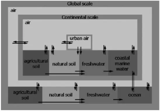
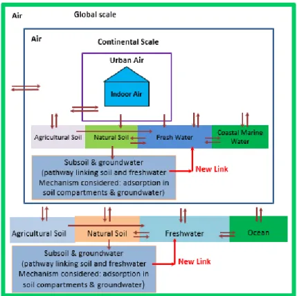
The USEtox model is set up to represent a global average continent within a global box, and with an urban zone nested (the contaminants can travel from one scale to the higher scale and vice versa) within the continental box without considering any spatial differentiation of location of the emission. The continental scale consists of six environmental compartments: urban air, rural air, agricultural soil, natural soil, freshwater and coastal marine water. The global scale has the same structure as the continental scale, but without the urban air compartment. The global compartment accounts for impacts outside the continental scale and it nests the continental scale. (Rosenbaum et al., 2008). Different compartments of the USEtox model is shown in Figure 2-3.

Figure 2-3 Different compartments in the USEtox model (Rosenbaum et al., 2008)

USEtox is a multi-compartment box model which calculates pollutant fate and effect to human health and ecosystem based on pollutant emission and exposure. The compartments systems and the mass flow rates are considered as homogeneous and well-mixed systems (Mackay, 2010; Rosenbaum et al., 2008).

(33)

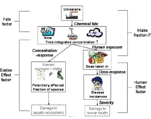
USEtox’s matrix framework is composed of a series of matrices combining fate with exposure and effect based on the matrix algebra developed by Rosenbaum, Margni, and Jolliet (2007). The links of the cause–effect chain are modelled using the matrices generated with the corresponding factors; the fate factor (𝐹𝐹̅̅̅̅) in day (which also denotes the persistence of the chemical), exposure (𝑋𝐹̅̅̅̅) in day−1 (only human toxicity) and effects (𝐸𝐹̅̅̅̅) in cases/kgintake for human toxicity or PAF (potentially affected fraction) m3/kg for ecotoxicity. This results in a set of scale-specific characterisation factors: (𝐶𝐹̅̅̅̅) in cases/ kgemitted, as shown in Equation 2. The impact pathways related with this calculation also depicted in Figure 2-4 (Henderson et al., 2011; Rosenbaum et al., 2008).

(34)

For ecotoxicity, the characterization factor is:

𝐶𝐹

̅̅̅̅ = 𝐹𝐹̅̅̅̅ × 𝐸𝐹̅̅̅̅

Equation 1

Fur human health, after the inclusion of exposure, the expression for characterization factor becomes:

𝐶𝐹

̅̅̅̅_{= 𝐹𝐹}̅̅̅̅_{× 𝑋𝐹}̅̅̅̅_{× 𝐸𝐹}̅̅̅̅ _{= 𝐸𝐹}̅̅̅̅_{× 𝑖𝐹}̅

Equation 2

The fate matrix (𝐹𝐹̅̅̅̅) and the exposure matrix (𝑋𝐹̅̅̅̅) together make the intake fraction matrix (𝑖𝐹̅ ) which denotes the part of the population that are exposed to that contamination. The fate factor (FF) is same for ecotoxicity and human toxicity (Rosenbaum et al., 2008).

Characterization factors (CFi freshwater ecotox, [PAF m3 day/kgemitted]) represent the freshwater ecotoxicological impacts of chemicals per mass unit of chemicals emitted in freshwater, where the impact is quantified as the potentially affected fraction (PAF) of species (PAF m3 day/kgemitted). For the context and brevity of this report, only the issues related to metal contamination in soil and freshwater are discussed.

The fate factor of metals are calculated in USEtox based on the total metal concentration. The CFs of metals were termed as interim (earlier) due to their relatively large uncertainties. However, in light of some recent improvements, there are new values of CF which are being added (Dong et al., 2014; Gandhi et al., 2010). Because of metals’ ability to speciate in the environment, only the bioavailable form of metals are actually considered to be doing harm to the ecosystem and human health. Therefore, according to the recommendation in the Clearwater consensus in 2010 by Diamond et al. (2010), the work of Gandhi et al. (2010), Plouffe et al. (2015) Owsianiak, Rosenbaum, Huijbregts, and Hauschild (2013) and Tromson, Bulle, and Deschênes (2017) are also important to mention in this context (Diamond et al., 2010; Gandhi et al., 2010; Plouffe et al., 2015; Rosenbaum et al., 2008).

(35)

For freshwater ecotoxicity, Gandhi et al. (2010) has included the bioavailability factor (BF) for Zn, Cu & Ni for freshwater system in CF calculation using WHAM 6 as a geochemical speciation model (this model was recommended by this workshop, Diamond et al. (2010)). Later the geographic variability was also included by Gandhi, Huijbregts, et al. (2011) in a Canadian context within the calculation of CFs since metal speciation depends on the ambient environmental chemistry and regional variability to a large extent (Diamond et al., 2010; Gandhi et al., 2010; Gandhi, Huijbregts, et al., 2011).

Gandhi, Huijbregts, et al. (2011) has compared the relative ranking of Cu, Ni and Zn in 24 Canadian ecoregions. DOC, pH, hardness and water residence time were chosen the influent landscape properties for 24 Canadian ecoregions (the ecoregions and metal hazard rankings were defined by LUCAS and ChemCAN models). CFs of these metals for freshwater were by up to three orders of magnitude and it also changed the relative ranking of metal hazard between these ecoregions. FFs were varied within two orders of magnitude, BFs within two orders of magnitude for Ni and Zn and four orders of magnitude for Cu, and EFs were varied within one order of magnitude (Gandhi, Huijbregts, et al., 2011).

Dong et al. (2014) extended this approach and standardized to 14 cationic metals (Al(III), Ba, Be, Cd, Co, Cr(III), Cs, Cu(II), Fe(II), Fe(III), Mn(II), Ni, Pb, Sr and Zn) using the seven freshwater archetypes categorized by Gandhi et al. (2010). Dong et al. (2014) concluded that spatial differentiation is important for metals like Al(III), Be, Cr(III), Cu(II) and Fe(III) which form stable hydroxyl complexes in slightly alkaline waters and for them CFs varied from 2.4 to 6.5 orders of magnitude. However, for Cd, Mn, Ni and Zn which are less pH dependent and have high partition coefficients, the spatial differences are not that important since new CFs only vary between 0.7 and 0.9 orders of magnitude. For other metals, the difference is less significant (around 0.4 orders of magnitude). When compared to current CFs, most of the newly calculated CFs are similar or higher and fall within the same two orders of magnitude (Dong et al., 2014).

Plouffe et al. (2015) has attempted to include metal speciation in terrestrial ecotoxicity in the calculation of CFs. Plouffe et al. (2015) has also used WHAM 6 as geochemical speciation model for soil metal speciation to define the bioavailable factors (BF). In the work that followed (Plouffe et al., 2016), had included the geographic variability into account along with speciation. The resulting aggregated terrestrial CF (4.70 PAF.m3.day/kg) is 62 times lower than the CFs calculated

(36)

using current methodology in USEtox (292 PAF.m3.day/kg). Again, using the value for soluble Zn, the aggregated global default CF value based on true solution Zn was (1.45 PAF.m3.day/kg) 201 times lower than the USEtox derived terrestrial CF (Plouffe, Bulle, & Deschênes, 2014 (Submitted); Plouffe et al., 2015).

Henderson, Dingsheng, and Jolliet (2012) had included speciation of Al on 12 EU water archetypes by Gandhi et al. (2010) in order to verify the Ecoinvent assumption that 100% Al is leached to groundwater from landfill and then to surface water. A conceptual model was constructed from the landfill site to the surface water and finally to a water treatment plant. WHAM 6 was used to perform the speciation of Al in this study. The results of including removal of Al in groundwater leads to a reduction in the fraction of a landfill emission transferred to surface water on the order of 10-4 to 10-6. This was assumed previously as 1 (100%) (Henderson et al., 2012).

In another recent study, a different approach was tested to obtain terrestrial ecotoxicity CFs for Cu and Ni by Owsianiak et al. (2013). In this study, empirical regression was used instead of using the computer models for soil speciation. A new factor (accessibility factor) was introduced in the definition of CF, although it was not mentioned in the recommendations of Clearwater consensus. The definition of accessibility was explained as similar with the concept of risk assessment of metals, the difference being the partitioning is in the nature instead of gastrointestinal environment. Owsianiak et al. (2013) used empirical regressions on 760 soil samples to determine BFs performed on experimental field data. Soil pH, organic carbon, Mg2+_{concentration in soil pore} water and soil clay content were chosen as influential properties to affect CF. Spatial variability of 3.5 and 3 orders of magnitude were observed between CFs for Cu and Ni (two orders of magnitude in a 95% interval) (Owsianiak et al., 2013).

All of the above mentioned studies by Owsianiak et al. (2013), Gandhi, Diamond, et al. (2011); Gandhi et al. (2010); Gandhi, Huijbregts, et al. (2011) and Plouffe et al. (2015) have proven that metal speciation including spatial/regional variability into account have a big influence on the CFs of metals for both soils and freshwater ecotoxicity impact categories.

(37)

2.3.1 The soil compartment in USEtox

For the model simplicity and also to limit huge data requirement, the soil compartment in USEtox is considered as one homogeneous layer having a depth of 10 cm. Soil in reality is a complex medium consisting of several different layers. Any chemical entering in the environmental compartments are considered to be instantly in equilibrium (Rosenbaum et al., 2008).

Soil compartment was distinguished as agricultural and natural. The agricultural soil is a fraction of total soil surface. Because the ecosystem is absent in the agricultural soil it is considered as part of the technosphere. This consideration allows to account for specific (e.g. pesticides & fertilizers) emissions occurring on agricultural soil only (Rosenbaum et al., 2008).

Four mechanisms of removal were considered from soil to surface water and the resulting flow of contaminants is a net result of competition between those four mechanisms. They are: degradation, volatilization, leaching to deeper layers of soil, and runoff to surface water. For surface water, only the chemical mass dissolved in (pore) water is modeled as available for taking part in physical and chemical processes (Henderson et al., 2011).

While considering the runoff, based on typical values for a temperate climate, USEtox assumes that half of net precipitation onto soils is evaporated, with the remaining half being split equally between surface water runoff (25%) and water infiltration (25%) through soil. The latter also implies that this transfer is limited to maximum of 50% from soil to surface water. However, chemicals can also be removed from the upper soil compartment via leaching to deep soil or groundwater, which removes mobile chemicals from the upper soil compartment. (Henderson et al., 2011).

Deposition to soil and fresh water in the global box is limited, since two thirds of the area in the global box is ocean. Wet removal by intermittent rain is responsible for the high fraction transferred to soil at low Kaw (air-water partition coefficient). The direct transfer from air to surface water (fa,w) also depends on Kaw, but deposition is limited by the fact that freshwater covers only 2.7% of the area in the continental box, and 0.9% in the global box. Therefore, the transfer from air to water is mostly via the soil compartment to water. However, Henderson et al. (2011) mentioned in the description of fate in USEtox that, this will only be important for substances with a high transfer to soil (log Kaw<−4 and t½(air)>1 day) and a high transfer fraction from soil to water

(38)

(log Koc<4). As a result, only a small subset of substances has an air to surface water transfer fraction higher than 20% (Henderson et al., 2011; Rosenbaum et al., 2008).

2.4 Metals in the environment

Metals are part of the earth’s crust and occur naturally in varying amounts in all environmental compartments. Metals cannot be created or destroyed. Human activities have increased the rate of redistribution of metals in the environmental compartments, particularly since the industrial revolution (Garrett, 2000). Emissions from metal mining, smelting and refining, power generation and solid-waste incinerators, manufacturing, and transportation sectors are some of the major sources of metals (Gandhi, 2011). After the emission of metals into the environmental compartments (air, water, soil, sediments) it is never decomposed or removed from the system and further they can bond with other anions and take varous oxidative states having different characteristics and toxicity (speciation).

2.4.1 Metal speciation and bioavailability

Speciation is a crucial parameter for metals since it governs mobility, environmental fate, their availability to living organisms and associated toxic effects. Metal speciation includes all physicochemical forms included in the total concentration of metal in the environment (Ge, 2002). When metal is released into the soil, it can be found in the various forms: dissolved, exchangeable fraction, organic fraction, inorganic fraction, residual fraction, fraction incorporated with organic material etc. These species coexist in the environment and may or may not in thermodynamic equilibrium (Fairbrother, Wenstel, Sappington, & Wood, 2007; Ge, 2002; N. M. Hassan, 2005). Metal speciation may also include metal different ionic forms. Indeed, some metals and metalloids including Cr, Cu and Hg can have several degrees of ionization, which affects their mobility, fate and toxicity in the environment. For example, trivalent Cr species have low toxicity as low bioavailability, since they tend to form strong organic and inorganic complexes. In contrast, hexavalent Cr species are highly soluble and easily absorbed by living organisms, where they can result in toxic effects (carcinogenic, teratogenic and mutagenic effects) (Daulton, Little, & Lowe, 2003; Williams, James, & Roberts, 2003).

(39)

After the Clearwater consensus, the definition of bioavailability was included in the calculation of characterization factors of metals, since metals are persistent and every form of metals were not considered harmful to human health and the ecosystem. The previous assumption of the inclusion of total metal concentration in the characterization factors was overestimating the impacts (Diamond et al., 2010).

The bioavailability Factor (BF) explicitly expresses the relationship between total dissolved and bioavailable chemical where the latter is assumed to be the truly dissolved concentration of the metal that does not include colloidally bound chemical (Diamond et al., 2010). So according to this definition, the BF can be written as:

𝐵𝐹 = [𝑀𝑒𝑡𝑎𝑙]𝑡𝑟𝑢𝑒 𝑠𝑜𝑙𝑢𝑡𝑖𝑜𝑛 [𝑀𝑒𝑡𝑎𝑙]𝑠𝑜𝑖𝑙

Equation 3

As mentioned in section 2.3, following the Clearwater consensus and after several attempts by various groups of researcers for including speciation into the LCA modeling (Dong et al., 2014; Gandhi et al., 2010; Henderson et al., 2012; Plouffe, 2015), the uncertainty was greatly reduced and it justified the need to take metal speciation under consideration.

2.4.1.1 Factors affecting metal speciation

The parameters that are most influential in speciation of heavy metals in soils are pH, temperature, redox potential, composition and concentration of other ions, organic matter (OM), cation exchange capacity (CEC), complexing agents (Carbonates), size and quantity of soil particles and the activity of microorganisms and plants. For most metal ions, pH plays an important role since it changes the metal’s solubility (aquatic & soil solution), adsorption (soil) and other parameters of influence (DOM and carbonate) for both soils and water (Sauvé, Hendershot, & Allen, 2000). At higher pH, adsorption of metals is increased and retained within the solid phase (Gandhi, 2011; Ge, 2002; Hellweg, Fischer, Hofstetter, & Hungerbühler, 2005).

Organic matter is also an important factor since it allows the formation of soluble metal complexes and can increase bioavailability of metals. Depending on other chemical parameters, it can also have opposite effects (Hellweg et al., 2005). Evidently, when most of the metal in solution is bound

(40)

to dissolved organic matter (DOM), any factor that influences solubility of organic matter will also affect metal solubility (Harter & Naidu, 1995; Sauvé et al., 2000)

Similar as in terrestrial environment, in aquatic systems, metal speciation, their bioavailability and mobility are influenced by pH, redox potential, organic complexes, and salinity (Achterberg, van den Berg, Boussemart, & Davison, 1997). Metals can form complexes with ligands from organic matter, and/or may be sorbed to suspended particulate matter (SPM) that later is transported to sediments (Carignan & Tessier, 1985). In general, pH and redox are among the most important factors that affect the mobility of sediment-bound metals in water (Wen & Allen, 1999). It is observed that lower pH increases metal dissolution (Förstner, Ahlf, Calmano, Kersten, & Salomons, 1986).

During seasonal changes when water transitions from oxic to anoxic conditions, mobility of Fe and Mn is increased due to dissolution of their oxide forms in the moderately reducing environments (Wen & Allen, 1999). Under strongly reducing conditions, metals such as Zn, Pb, Cu, and Cd are immobilized because they precipitate as metal sulphides. Conversely, these metals can be released from their metal sulphides as conditions shift from reducing to oxidizing as oxygen is introduced or during seasonal changes. (Carignan & Tessier, 1985; Hamilton‐Taylor, Davison, & Morfett, 1996).

In weakly buffered sediments, a change in redox potential can change water pH, which may change the mobility of most metals (de CARVALHO, ZANARDI, BURATINI, LAMPARELLI, & MARTINS, 1998). Thus, metals deposited in sediments are not necessarily permanently immobilized. It would be safe to consider that they are rather remobilized through diagenetic processes (Carignan & Tessier, 1985) involving biological and chemical agents and by physical movement (Diamond, 1995; Förstner et al., 1986).

Metal in the soluble phase of soil can be taken up by plants where it may be stored and then returned to soil upon plant death. Metals can be transported to nearby surface aquatic systems through runoff and and can also leach to groundwater thereby seemingly ‘lost’ from soils. Surface soils and groundwater could be a major source of metals to aquatic systems (Gandhi, 2011).

2.4.2 Metal speciation calculation with WHAM

WHAM (Windermere Humic Aqueous Model), is an equilibrium speciation model specifically designed to calculate equilibrium chemical speciation in environmental media. The model is