OPTIMIZATION OF UNDERGROUND STOPE WITH NETWORK FLOW METHOD
XIAOYU BAI
D´EPARTEMENT DES G´ENIES CIVIL, G´EOLOGIQUE ET DES MINES ´
ECOLE POLYTECHNIQUE DE MONTR´EAL
TH`ESE PR´ESENT´EE EN VUE DE L’OBTENTION DU DIPL ˆOME DE PHILOSOPHIÆ DOCTOR
(G ´ENIE MIN ´ERAL) AO ˆUT 2013
c
´
ECOLE POLYTECHNIQUE DE MONTR´EAL
Cette th`ese intitul´ee :
OPTIMIZATION OF UNDERGROUND STOPE WITH NETWORK FLOW METHOD
pr´esent´ee par : BAI Xiaoyu
en vue de l’obtention du diplˆome de : Philosophiæ Doctor a ´et´e dˆument accept´ee par le jury d’examen constitu´e de :
M. JI Shaocheng, Ph.D., pr´esident
M. MARCOTTE Denis, Ph.D., membre et directeur de recherche M. SIMON Richard, Ph.D., membre et codirecteur de recherche M. GAMACHE Michel, Ph.D., membre
ACKNOWLEDGMENTS
Even today, it still seems unrealistic to me that, a bad student who used to struggle and prey to pass math courses is doing his PhD, on a project quite related to math. In fact this is the true history behind this dissertation. I would like to take this opportunity to thank various people who helped me to achieve this work.
First of all, I would like to express my deep gratitude to Prof. Denis Marcotte, for accep-ting me, guiding me, encouraging me, and funding me. Working with him, I start to discover the fun of geostatistics and Matlab. No need to mention his key contribution to this disser-tation.
I am also grateful to Prof. Richard Simon, who provides very important and practical advices on mining engineering aspect.
I sincerely acknowledge China Scholarship Council, for offering me the scholarship, brin-ging me good chance to study in Canada.
I also want to thank my colleagues and friends in the lab, Carole Kaouane, Pejman Shamsipoor, Martine Rivest, Abderrezak Bouchedda, Eric Chou, Catherine Chou, Shengsi Sun, Pengzhi Zhao, and Fidele Yrro. I enjoy the time of sharing knowledge and entertaining.
Finally, many thanks to my wife Min Liang for her invaluable support, and my parents in half a planet away for their constant encouragement.
R´ESUM´E
La th`ese pr´esente une s´erie d’algorithmes originaux visant `a optimiser la g´eom´etrie de chantiers souterrains en 3D, typiquement pour la m´ethode d’abattage par sous-niveaux (ou m´ethode des longs trous). Les algorithmes propos´es s’inspirent des m´ethodes efficaces d’op-timisation ayant ´et´e d´evelopp´ees pour les mines `a ciel ouvert. La cl´e de l’adaptation de cette m´ethode pour la m´ethode des longs trous est de reconnaˆıtre que la chemin´ee verticale (ou monterie), servant `a initier un chantier, joue un rˆole similaire `a la surface dans les mines `a ciel ouvert. Un syst`eme de coordonn´ees cylindriques est d´efini autour de la monterie. Les va-leurs ´economiques des blocs dans ce syst`eme sont d´etermin´ees `a partir des donn´ees en forage. Les angles limites pour le toit et le plancher sont contrˆol´es par les liens entre les blocs en coupe verticale. La longueur de chantier est contrˆol´e dans le plan horizontal, `a l’aide de deux param`etres : 1) R, la distance horizontale maximale entre un bloc et la chemin´ee et 2) yR,
la largeur minimale de l’enveloppe cr´e´ee pour exploiter le bloc se trouvant `a cette distance maximale. La hauteur du chantier est d´etermin´ee par l’extension de la monterie, laquelle limite aussi les liens dans le plan vertical. L’ensemble des liens et des blocs constitue un r´eseau. Le r´eseau est compl´et´e par deux noeuds fictifs, la source et le puits. En maximisant le flux partant de la source vers le puits, on identifie le chantier optimal. Le chantier obtenu est optimal cependant conditionnellement `a la monterie ´etudi´ee (localisation et extension), la discr´etisation adopt´ee et les liens repr´esentant les contraintes de pentes. Le probl`eme revient alors `a d´eterminer les param`etres de la monterie qui maximisent le profit. Pour ce faire, on utilise une m´ethode de type g´en´etique permettant d’explorer des solutions vari´ees et surtout de s’´echapper d’optimums locaux. La m´ethode est appliqu´ee sur plusieurs gisements et les r´esultats sont compar´es `a ceux de la m´ethode du chantier flottant (“floating stope”). La m´ e-thode propos´ee d´emontre sa sup´eriorit´e sur ces exemples.
La m´ethode est ensuite g´en´eralis´ee `a l’optimisation d’un chantier ou de chantiers compre-nant plusieurs monteries verticales. `A nouveau l’algorithme g´en´etique est utilis´e. L’ensemble des sous-chantiers associ´es aux diverses monteries sont fusionn´es dans l’espace cart´esien pour former un seul chantier global. Des gisements simul´es et un gisement r´eel montrent que la solution `a plusieurs monteries permet de g´en´erer un profit sup´erieur `a la solution optimale pour une seule monterie. Le gain obtenu avec plusieurs monteries est particuli`erement per-ceptible pour le cas de gisements courbes ou pr´esentat des zones distinctes de min´eralisation.
eve-loppment des galeries de sous-niveaux pour la m´ethode des longs trous avec forages verticaux parall`eles. L’extension de la galerie d´epend en effet de l’extension du chantier. Il y a donc un gain `a optimiser ces deux ´el´ements conjointement. Ceci est r´ealis´e par l’ajout d’un lien de pr´ec´edence entre les blocs situ´es sur les sous-niveaux et les blocs associ´es aux monteries situ´es sur la mˆeme ligne verticale. On montre avec des exemples que l’algorithme avec les galeries fournit un profit de chantier sup´erieur `a la solution sans les galeries. De plus les solutions obtenues montrent des chantiers plus petits que lorsque le coˆut de d´eveloppement des galeries est ignor´e.
Une ´etude de sensibilit´e des param`etres du mod`ele indique que la discr´etisation du sys-t`eme cylindrique doit ˆetre suffisamment fine. L’algorithme g´en´etique apparaˆıt assez robuste aux choix des divers autres param`etres, du moins pour le cas type ´etudi´e. Par mesure de pr´ e-caution, il est recommand´e d’appliquer l’algorithme `a partir de plusieurs solutions initiales diff´erentes. ´Egalement, il vaut mieux initier l’algorithme avec des valeurs faibles du param`etre R, le rayon maximal de chantier `a partir d’une monterie, et laisser croˆıtre celui-ci au gr´e de mutations ou autrement. Un probl`eme li´e `a ce param`etre est qu’au del`a d’un certain R, selon les valeurs prises par les autres param`etres, la fonction objectif ne peut plus fluctuer. La meilleure fa¸con de traiter ce param`etre demeure `a d´eterminer.
Les m´ethodes propos´ees sont applicables `a la m´ethode d’abattage par sous-niveaux. Elles donnent des r´esultats int´eressants pour les gisements sub-horizontaux ou sub-verticaux. Pour les gisements inclin´es, des d´eveloppements devront ˆetre r´ealis´es. L’extension `a d’autres m´ e-thodes de minage est possible mais des adaptations seront sans doute requises. N´eanmoins, l’approche propos´ee constitue un pas important vers l’optimisation exacte des chantiers d’abattage en souterrain et marque un progr`es significatif par rapport aux m´ethodes exis-tantes, en particulier par la fa¸con dont l’approche permet de tenir compte explicitement des contraintes mini`eres.
ABSTRACT
The dissertation presents a series of algorithms to optimize the underground stope geome-try in 3D, typically for sublevel stoping method or longhole stoping. The proposed algorithms are based on network flow method, an effective technique applied in open pit optimization. The key to adapt this method to underground mining is to recognize that the vertical raise to initiate a stope plays a similar role to the surface in open pit mining. Accordingly, a cylin-drical coordinate system starting from the raise is introduced to redefine a ore block model. This facilitate the manipulation of geometric constraints. The slope limits of hanging wall and footwall are controlled by the links between the blocks in vertical section. The width of stope is controlled in horizontal plane, by defining two parameters: 1) R, the maximum dis-tance to mine a block from raise, and 2) yR, the minimum width of envelope created to mine
the farthest block. The height of stope is defined by the raise extension which limits the links in the vertical section. The blocks and links constitute a network flow graph. Solving the graph with efficient maximum flow method yields an optimal stope conditional to the spec-ified raise. This is the core of proposed methods, an optimal stope generator for given raise parameters. With the stope generator, the global optimization of raise parameters produces a global optimal stope. The algorithm using a single raise is suitable for the relatively small sub-vertical ore bodies. It is shown to provide better results than floating stope algorithm in several scenarios tested.
The algorithm using multiple raises is also developed still using the genetic algorithm. In the stope generator with multiple raises, the sub-stopes independently created from each raise are converted back to Cartesian system, and then merged to form an overall stope. The parameters of raises are also adjusted accordingly. The multiple raises solution can provide good heuristic stope. The test cases show that the multiple raises solution produces higher profit than single raise solution, especially for curved deposits and large deposits.
Moreover, the framework of stope optimizer is modified to incorporate sub-level drift in stope optimization, typically for longhole vertical parallel drilling pattern. The layers of drift blocks are identified according to the levels of given raise. The dependency relation of the blocks of drift and the blocks for stoping are expressed by the links in vertical section. Adding the new links to previous graph results in a stope with drift jointly optimized. It is shown that the algorithm with drift involved provides higher stope profit and smaller stopes than the solution without integrating drift.
Sensitivity study of parameters to the method indicates that the discretization of block model in cylindrical system should be fine enough. The genetic algorithm appears quite ro-bust to the choice of other parameters, at least for the typical deposit used in the sensitivity analysis. As a precaution, it is recommended to apply the algorithm from several different initial solutions. Also, it is better to initiate the algorithm with low values of the parameter R, the maximum radius of a stope from a raise, to let it increase by mutation or other ways. A problem with the parameter R is that with certain other parameters, and R large enough, the objective function does not change anymore with R. The best way to deal with this setting remains to be determined.
The proposed methods are applicable to the sublevel stoping method. They give interest-ing results for the sub-horizontal or sub-vertical fields. For inclined deposits, developments will be realized. The extension to other mining methods is possible but adaptations will undoubtedly be required. However, the proposed approach is an important step towards the exact optimization of underground stopes and marks a significant improvement over existing methods, in particular by the way the approach allows explicit consideration of mining con-straints .
TABLE OF CONTENTS DEDICATION . . . iii ACKNOWLEDGMENTS . . . iv R´ESUM´E . . . v ABSTRACT . . . vii TABLE OF CONTENTS . . . ix
LIST OF TABLES . . . xii
LIST OF FIGURES . . . xiii
LIST OF INITIALS AND ABBREVIATIONS . . . .xviii
LIST OF APPENDICES . . . xx
CHAPTER 1 INTRODUCTION . . . 1
1.1 Basic concepts and research problems . . . 1
1.2 Objectives of the research . . . 2
1.3 Contributions of the thesis . . . 2
1.4 Structure of the thesis . . . 3
CHAPTER 2 LITERATURE REVIEW . . . 4
2.1 Ore reserve modeling . . . 4
2.2 Optimization for underground stope design . . . 4
2.2.1 Dynamic programming . . . 5
2.2.2 Mathematical morphology approach . . . 5
2.2.3 Floating stope technique . . . 6
2.2.4 The maximum value neighborhood method . . . 6
2.2.5 Branch and bound technique . . . 7
2.2.6 Octree division approach . . . 7
2.2.7 Simulated annealing . . . 7
2.3 Pit optimization . . . 8
CHAPTER 3 ARTICLE 1 : UNDERGROUND STOPE OPTIMIZATION WITH
NET-WORK FLOW METHOD . . . 10
3.1 Abstract . . . 10
3.2 Introduction . . . 10
3.3 Methods . . . 12
3.3.1 Economic block model . . . 12
3.3.2 Graph theory based optimization for open pit . . . 13
3.3.3 Analogy with sublevel stoping method . . . 14
3.3.4 Ore block model in cylindrical coordinates . . . 15
3.3.5 Graph for stope optimization . . . 15
3.3.6 Algorithm . . . 17
3.3.7 Floating stope technique . . . 20
3.4 Results . . . 21
3.4.1 Test on synthetic ore block models . . . 21
3.4.2 Test on real deposit . . . 24
3.4.3 Comparison with floating stope technique . . . 27
3.5 Discussion . . . 27
3.6 Conclusions . . . 33
3.7 Acknowledgement . . . 34
REFERENCE . . . 35
CHAPTER 4 ARTICLE 2 : A HEURISTIC SUBLEVEL STOPE OPTIMIZER WITH MULTIPLE RAISES . . . 37
4.1 Abstract . . . 37
4.2 Introduction . . . 37
4.3 Methods . . . 39
4.3.1 Stope optimization with single raise . . . 39
4.3.2 Stope optimization with multiple raises . . . 43
4.4 Results . . . 48
4.4.1 Parameters in the algorithm . . . 48
4.4.2 Test results : multiple raises vs. single raise . . . 49
4.5 Discussion . . . 54
4.6 Conclusions . . . 55
4.7 Acknowledgement . . . 55
CHAPTER 5 ARTICLE 3 : INCORPORATING DRIFT IN LONG-HOLE STOPE
OP-TIMIZATION USING NETWORK FLOW ALGORITHM . . . 58
5.1 Abstract . . . 58
5.2 Introduction . . . 58
5.3 Methodology . . . 60
5.3.1 Economical function of longhole stoping . . . 60
5.3.2 Stope optimization algorithm . . . 61
5.3.3 Comparative method . . . 63
5.4 Results . . . 65
5.4.1 Data and parameters in the algorithm . . . 65
5.4.2 Test results . . . 65
5.5 Discussion . . . 69
5.6 Conclusions . . . 70
5.7 Acknowledgement . . . 70
REFERENCE . . . 71
CHAPTER 6 PARAMETER SELECTION AND SENSITIVITY ANALYSIS . . . 73
6.1 Recent adjustment of GA . . . 73
6.1.1 Parents selection . . . 73
6.1.2 Genetic operator . . . 74
6.1.3 Effect of different raise parameters to evolution of GA . . . 74
6.2 Sensitivity test of the optimization parameters . . . 75
6.2.1 Discretization in the block model of cylindrical system . . . 75
6.2.2 Impact of randomness of initial population . . . 76
6.3 The size of initial population . . . 77
6.4 The number of offspring in new generation . . . 77
6.5 Mutation Rate . . . 78
6.6 The number of parents to mate . . . 78
6.7 Discussion and summary . . . 80
CHAPTER 7 GENERAL DISCUSSION AND CONCLUSION . . . 81
7.1 Conclusion . . . 81
7.2 Limitations and potential improvements in future . . . 81
REFERENCE . . . 83
LIST OF TABLES
Tableau 2.1 Comparison between the existing stope optimization algorithms . . . . 5
Tableau 3.1 Geometric and design parameters, discretization, and optimized raise parameters. . . 22
Tableau 3.2 Economical evaluation of the case studies. . . 22
Tableau 4.1 Geometric and design parameters, discretization, and optimized raise parameters. . . 50
Tableau 4.2 Economical evaluation of the case studies. . . 54
Tableau 5.1 Ore grade model, discretization, and economic, geometric and design parameters . . . 66
Tableau 5.2 Optimized raise parameters . . . 66
Tableau 5.3 Economical evaluation of the case studies. . . 66
LIST OF FIGURES
Figure 1.1 Common geometric constraints of a stope . . . 2 Figure 3.1 Vertical section showing typical arcs for open pit optimization in 2D. . 15 Figure 3.2 Block model under cylindrical coordinates a), and typical arcs in
ver-tical section in proposed method b). . . 16 Figure 3.3 Horizontal plane showing blocks and links defined in the cylindrical
system a) and corresponding blocks and links in the Cartesian system b). Shaded blocks represents blocks to be removed to get access to block A. Trace of the envelopes defined by the lateral links (function of K and R) in the cylindrical system c) as they appear in the Cartesian system d). Envelopes are computed with Eq. 3.5. . . 18 Figure 3.4 K = ∆θ
∆r parameter (degree/m) as a function of control parameters
R (reference distance to raise) and ymax
R stope width parameter. For
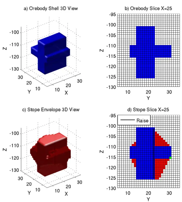
example, a block at 20 m from the raise with a maximum width of 6 m necessitates a discretization approximately K = 1.7 degree/m with a single lateral link on both sides of the radial link as in Fig. 3.3. . . . 19 Figure 3.5 Case 1, simulated ore model and stope by network flow method : a)
3D-view of the orebody, b) yz vertical section of the orebody at x=25, c) 3D view of the optimized stope, d) yz vertical section of the optimized stope at x=25 showing ore in stope (blue), waste in stope (red), and ore out of stope (green). Design parameters as given in Table 3.1 . . . . 23 Figure 3.6 Case 2, simulated ore model and stope by network flow method : a)
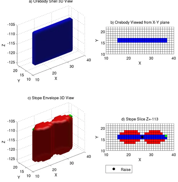
3D-view of the orebody, b) xy horizontal section of the orebody at z=-113, c) 3D view of the optimized stope, d) xy horizontal section of the optimized stope at z=-113 showing showing ore in stope (blue), waste in stope (red), and ore out of stope (green). Design parameters as given in Table 3.1. . . 25 Figure 3.7 Case 3, simulated ore model and stope by network flow method : a)
3D-view of the orebody, b) yz vertical section of the orebody at x=20, c) 3D view of the optimized stope, d) yz vertical section of the optimized stope at x=20 showing ore in stope (blue), waste in stope (red). Design parameters as given in Table 3.1. . . 26
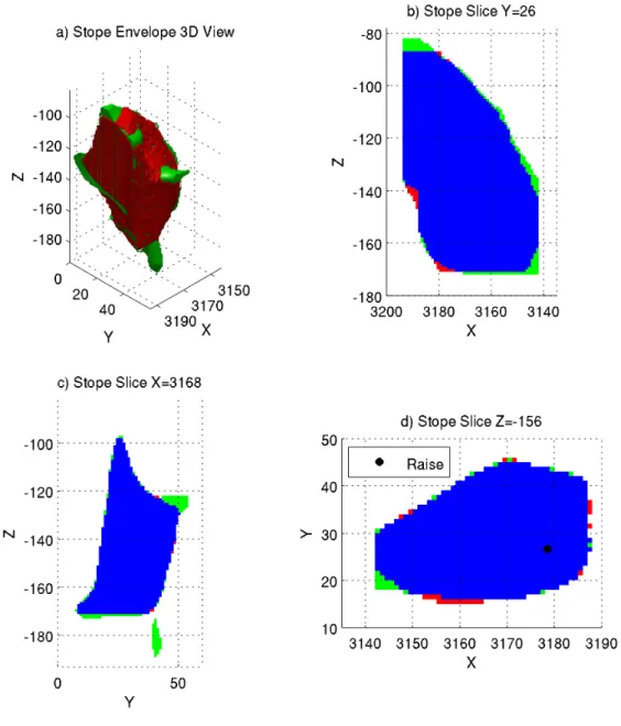
Figure 3.8 Case 4, real ore deposit : a) 3D-view of the orebody, b) xz vertical section of the orebody at y=26, c) yz vertical section at x=3168 and d) xy horizontal section at z=-156. . . 28 Figure 3.9 Case 4, optimized stope for the real deposit by the network flow
al-gorithm : a) 3D-view of the stope (red) and of the ore out of stope (green), b) xz vertical section of the stope at y=26, c) yz vertical sec-tion at x=3168 and d) xy horizontal secsec-tion at z=-156. For b), c) and d), ore in stope (blue), waste in stope (red), and ore out of stope (green). Design parameters as given in Table 3.1. . . 29 Figure 3.10 Inner stope for case 4 produced by floating stope technique : a) 3D-view
of the stope (red) and of the ore out of stope (green), b) xz vertical section of the stope at y=26, c) yz vertical section at x=3168 and d) xy horizontal section at z=-156. For b), c) and d), ore in stope (blue), waste in stope (red), and ore out of stope (green). . . 30 Figure 3.11 Outer stope for case 4 produced by floating stope technique : a) 3D-view
of the stope (red) and of the ore not included in the stope (green), b) xz vertical section of the stope at y=26, c) yz vertical section at x=3168 and d) xy horizontal section at z=-156. For b), c) and d), ore in stope (blue), waste in stope (red), and ore out of stope (green). . . 31 Figure 4.1 Block model under cylindrical coordinates a), and typical arcs in
ver-tical section in the proposed method b). . . 41 Figure 4.2 Horizontal plane showing a) blocks and links defined in the cylindrical
system and b) corresponding blocks and links in the Cartesian system. Shaded blocks represents blocks to be removed to get access to block A. Trace of the envelopes defined by the lateral links in the cylindrical system c) as they appear in the Cartesian system d). . . 42 Figure 4.3 Illustration of possible problems with one raise : a) In a horizontal
section, the envelope from A to the raise includes a large quantity of waste ; b) In a vertical section, waste has to be mined in the upper part due to the network associated to the single raise. . . 44 Figure 4.4 Conceptual model of stope generator with multiple raise in horizontal
section a) Two ore models in cylindrical coordinates, one for each raise, are established ; b) and c) first and second sub-stopes in cylindrical coordinate obtained by maxflow method on the two separate networks ; d) and e) the sub-stopes b) and c) converted on the Cartesian grid ; f) the final stope in Cartesian grid from d) and e). . . 45
Figure 4.5 Genetic algorithm diagram to search for the best raises’ parameters. . . 47 Figure 4.6 Case 1, simulated ore model and created stopes : a) 3D-view of the
orebody, b) x-y horizontal section of the orebody at z=-120, c) 3D view of the optimized stope with a single raise, d) x-y horizontal section of the single raise stope at z=-120, showing ore in stope (blue), waste in stope (red), and ore out of stope (green). e) 3D view of the optimized stope by multiple raises, f) x-y horizontal section of the multiple raises’ stope at z=-120. Raises in black. Design parameters as in Table 4.1. . . 51 Figure 4.7 Case 2, simulated ore model and created stopes : a) 3D-view of the
orebody, b) x-y horizontal section of the orebody at z=-120, c) 3D view of the optimized stope with a single raise, d) x-y horizontal section of the single raise stope at z=-120, showing ore in stope (blue), waste in stope (red), and ore out of stope (green). e) 3D view of the optimized stope by multiple raises, f) x-y horizontal section of the multiple raises’ stope at z=-120. Raises in black. Design parameters as in Table 4.1. . . 52 Figure 4.8 Case 3, test with a real ore deposit : a) 3D-view of the orebody, b)
y-z vertical section of the orebody at x=3130, c) x-y horizontal section at z=-424 ; d) 3D view of the optimized stope with a single raise, e) y-z vertical section at x=3130, f) x-y horizontal section at z=-424 ; g) optimized stope with multiple raises, h) y-z vertical section at x=3130, i) x-y horizontal section at z=-424 ; in d) and g), stopes are in red, ore out of stope is in green. e),f), h) and i), ore in blue, waste in red, and ore out of stope in green, raises in black. Design parameters as in Table 4.1. . . 53 Figure 5.1 Block model under cylindrical coordinates a), and typical arcs in
ver-tical section in proposed method b). Arcs to integrate drift in stope optimization c) . . . 63 Figure 5.2 Horizontal plane showing blocks and links defined in the cylindrical
system a) and corresponding blocks and links in the Cartesian system b). Shaded blocks represent blocks to be removed to get access to block A. Trace of the envelopes defined by the lateral links (function of K and R) in the cylindrical system c) as they appear in the Cartesian system d). . . 64
Figure 5.3 Case 1, simulated ore model and created stopes : a) 3D-view of the orebody, b) yz vertical section of the orebody at x=20, c) xy horizontal section at z=-130 ; d) optimized stope and drift with traditional method view in 3D, e) yz vertical section at x=20, f) xy horizontal section at z=-130 ; g) optimized stope and drift with proposed method view in 3D, h) yz vertical section at x=20, i) xy horizontal section at z=-130 ; For the 3D view of stopes in d) and g), stopes are marked light meshes, and drifts are marked in dark squares. For stope slices in e),f),h) and i), stope(shaded area), drifts(square) ; waste in stope(+), and ore out of stope (x). Raises are marked in black lines with dots. Design parameters are given in Table 5.1. . . 67 Figure 5.4 Case 2, test with real ore deposit : a) 3D-view of the orebody, b) xz
vertical section of the orebody at x=3168, c) xy horizontal section at z=-144 ; d) optimized stope and drift with traditional method view in 3D, e) xz vertical section at x=3168, f) xy horizontal section at z=-130 ; g) optimized stope and drift with proposed method view in 3D, h) xz vertical section at x=20, i) xy horizontal section at z=-144 ; For the 3D view of stopes in d) and g), stopes are marked light meshes, and drifts are marked in dark squares. For stope slices in e),f),h) and i), stope(shaded area), drifts(square) ; waste in stope(+), and ore out of stope (x). Raises are marked in black lines with dots. Design parameters are given in Table 5.1. . . 68 Figure 6.1 Deposit model for parameter analysis : a) projection on X-Z plane, b)
projection on X-Y plane. Ores are marked in brown. . . 76 Figure 6.2 Impact of ∆r on the stope profit . . . 77 Figure 6.3 a) The distribution of stope profit with different initial raises ; b) The
locations of optimized raises (in white paired dots) and the correspon-ding R with different initial raises ; The real optimal raises are shown in yellow. The brown areas are the orebodies projected on X-Y plane. . 78 Figure 6.4 a) The viability of stope profit with different sizes of initial population ;
b) The viability of stope profit with different number of new individuals in a generation ; c) Influence of mutation rate ; d) Influence of number of parents to mate . . . 79 Figure A.1 A simple block model in 2D. The economic value of the block are noted
at center. The positives blocks are filled in gray. The block numbers are labeled in top-left corner. . . 88
Figure A.2 Network flow model for a simple 2D open pit optimization. The nodes are the circles. The capacities are labeled aside the links. The optimal solution is represented by the gray circles. . . 89
LIST OF INITIALS AND ABBREVIATIONS
Maxflow Maximum Flow
MVN Maximum Value Neighborhood
STP-D Stope Dimension
FWA Foot Wall Angle
HWA Hanging Wall Angle
SOS2 Type-Two Special Ordered Sets
MIP Mix Integer Programming
LGA Lerchs–Grossmann Algorithm
GA Genetic Algorithm
CNFV Cumulative Normalized Fitness Value
G a graph
V vertices in a graph
A arcs in a graph
p economic value of a block
d density of rock
v volume of block
g average grade of a block
r recovery rate
f unit metal price
c the unit cost of processing and mining
c(x) the unit cost of processing and mining varying with raise location x
N the number of blocks in ore block model
Γi the subset of immediate successor nodes to node i
s a source node in a network flow graph t a sink node in a network flow graph
(r, θ, z) the parameters in cylindrical coordinates (radial distance, azimuth, elevation)
(∆r, ∆θ, ∆z) the unit block in cylindrical coordinates
K the ratio ∆θ/∆r of block unit at tangential direc-tion and radial direcdirec-tion
R the maximum distance from raise to include a block in stope
yRmax or yR stope width parameter
(xi, yi, zib, zit, Ri) the parameters of a raise noted by i : xi and yi,
the coordinates in horizontal section ; zib and zti, its bottom and top elevation ; Ri is the maximum
distance a block can be from the raise X the parents in genetic algorithm Xnew the new offspring in genetic algorithm
β the random weight vector of the gene contributions from parents
α0 the indicator of gene mutation of a new individual σ the extent of mutation of a gene
LIST OF APPENDICES
APPENDIX A AN EXAMPLE OF APPLICATION OF MAXFLOW METHOD IN MINING OPTIMIZATION . . . 87
CHAPTER 1
INTRODUCTION
1.1 Basic concepts and research problems
In underground mining, the stope layout is a significant component of mine design. A successful stope design requires the deposit to be precisely modeled, the geological setting well grasped, and the mining method adequately selected. The stope, enclosing the ores or rocks to be mined, should produce as much economic profit as possible, yet it must be rea-listic and safe from a mining point of view. The economic outcome is the primary concern of stope design. In a mine project, even 5% discrepancy of profit from different stopes can represent a considerable amount of money(Whittle, 1989). On the other hand, the dimensions and shapes of stope are subjected to constraints due to 1) the mining method adopted and 2) the geotechnical considerations. The limits on stope dimensions and walls vary with different mining methods, such as cut-and-fill method and sublevel stoping method. Stope walls should also account for the in-situ rock proprieties such as rock strength and in-situ stress tensor, and local structures, such as faults and joints. In stope design, these complex constraints are characterized by geometric parameters, including maximum and minimum stope width and height, hanging wall and foot wall angle limits, as illustrated in Figure 1.1.
In general, the stope optimization is deemed as a constrained optimization problem, which is to find the highest profit stope subject to the geometric constraints. Viewing the stope opti-mizer as a black box, the input data to the box is the ore block model quantifying the mineral content or economic profit of block volumes on regular grids. The output is the geometry of stope indicating the blocks to be mined.
Despite the conceptual simplicity, the stope optimization is a challenging task. Contrary to open pit where efficient algorithms providing optimal solutions exist, the rare stope design algorithms proposed in the literature are rather crude heuristics that do not allow to include easily the mining constraints and for which the gap of optimality is unknown, nor even asses-sed. Moreover, accessory mining components such as drift and raise are commonly handled posteriorly to the stope design. However, in some mining methods, such as sublevel stoping with parallel longholes, the drift depends on the stope position and the development cost is non-negligible, thus should be accounted directly in the stope optimization.
Figure 1.1 Common geometric constraints of a stope
1.2 Objectives of the research
In light of the above problems in stope optimization, this thesis aims to develop new stope optimization algorithms, typically for sublevel stoping method. The algorithms are expected to achieve the following tasks :
1. Seek to produce optimal stope geometry ;
2. Incorporate comprehensively the geometric constraints in 3D ; 3. Have adaptability to various deposit scenarios.
4. Integrate drift in optimization.
1.3 Contributions of the thesis
By reaching the thesis objectives, the following main contributions will be achieved : 1. The development of the first stope optimizer that is proven optimal, for small deposits
exploited by a single vertical raise, and under specified mining constraints about wall angles, stope height and stope width ;
2. The development of an efficient heuristic for the multiple raises case allowing to extend the applicability of the stope optimizer to a wider class of deposits, larger, with more complex shapes, and possibly exploited on multiple sublevels ;
3. The development of a stope optimizer and heuristic allowing to include costs of drifts directly into the optimization.
These contributions apply to the currently most prevailing underground mining method : the sublevel stoping (Haycocks and Aelick, 1992). They are however restricted to subhori-zontal or subvertical deposits. The case of inclined deposits requires nontrivial adaptation to the proposed method that are not considered in this thesis (Bai et al., 2013b,a)
1.4 Structure of the thesis
This thesis consists of seven chapters. The first chapter provides a general view of un-derground stope optimization, and states the purposes of research. Chapter 2 reviews the state-of-art of stope optimization and relevant subjects. From chapter 3 to chapter 5, three progressive research articles are presented. Chapter 3 presents the first article entitled “Under-ground stope optimization with network flow method” published in Computer & Geoscienses, which is the basic building block for the stope optimization. It shows how the network flow open pit approach can be translated for underground optimization by the use of a cylindri-cal coordinate system defined around the raise. In Chapter 4, the second paper describes a generalization of the single raise optimizer of Chapter 3 for the case of multiple raises. The generalization allows to better represent large deposits or deposits with more complex shapes. A genetic algorithm (GA) is used in conjunction with the single raise stope opti-mizer to provide heuristic solutions that improve over the single raise optimal solution, yet respecting mining constraints. In Chapter 5, an article accepted by 2013 APCOM conference introduces a method to incorporate drift in long-hole stope optimization based on the pre-viously proposed framework. The joint optimization with the cost of drift level provides a stope with higher overall profit than the traditional methods, which handles the drift and stope separately. Chapter 6 presents a short sensitivity study of the GA to the choice of the different parameters. Chapter 7 summarizes the contributions and highlights of the thesis, addresses the limitations, and provides suggestions for future researches. An illustration of the open pit problem is presented in the Appendix.
CHAPTER 2
LITERATURE REVIEW
The state-of-the-art stope optimization and relevant subjects are reviewed in three parts. First, ore reserve modeling techniques are briefly overviewed, as a model quantifying the spa-tial distribution of ore grade is a premise for stope design. The second part surveys the stope optimization methods. The third part reviews the pit optimization techniques. The open pit optimization techniques are adapted to stope designs in the next chapter. Similarity of pit design and stope design is highlighted.
2.1 Ore reserve modeling
To optimize the design of stopes, an ore reserve model is needed. Modeling a ore grade distribution is the process of estimating the mineral content onto grids in 2D or 3D according to known discrete borehole data and local geological informations. This work usually resorts to geostatistical techniques (David, 1988; Journel and Huijbregts, 1978; Chil`es and Delfiner, 1999). The variogram, an essential geostatistical tool, is used to characterize the spatial dis-tribution of minerals. The in-situ geological interpretation also offers important guidance on position and continuity of ore body. The Kriging is the most common estimator and interpo-lator, which can provide a smooth map in average sense without bias. Conditional simulation techniques provide another options aimed to model the uncertainty of mineralizations, by producing a series of maps each showing a similar variogram to the real field (Journel, 1974; Dimitrakopoulos, 1998; Dowd and Dare-Bryan, 2005) and conditioned by the available in-formation. Applying economic functions on an ore grade model, an economic model can be obtained (Lane, 1988; Rendu, 2008), with which the cost and benefit of decisions on mining design, and their uncertainty, can be straightforwardly evaluated.
2.2 Optimization for underground stope design
The state-of-the-art on underground stope optimization was reviewed by Ataee-Pour (2005) and Alford et al. (2007). To the best of our knowledge, there are seven methods publi-shed on this topic, including : the dynamic programming, mathematical morphology method, floating stopes technique, maximum value neighborhood method (MVN), branch and bound
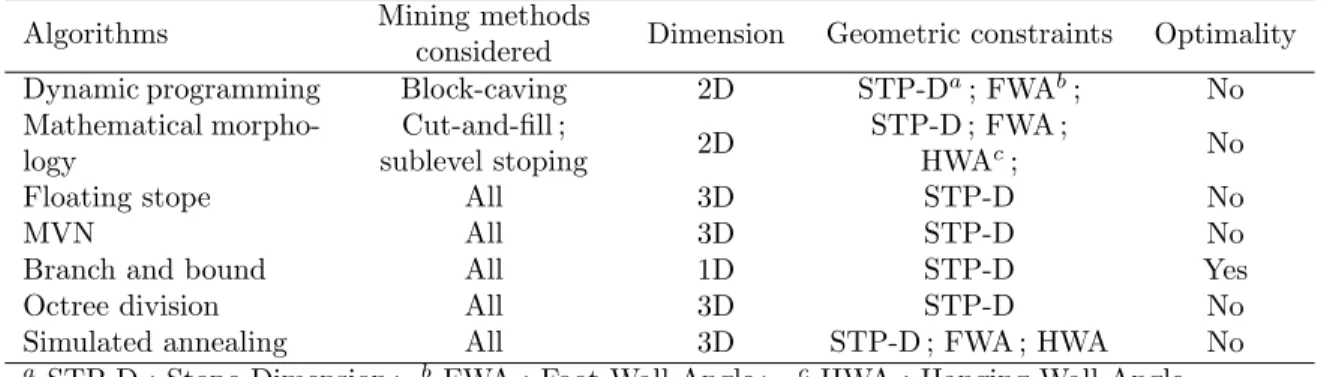
technique, octree division approach and simulated annealing. To compare these methods, the following important factors should be considered : is real optimal solution guaranteed ; does the method applies to all mining methods ; are all geometric constraints integrated ; is the method fully 3D. These properties of the optimizers are illustrated in Table 2.1. The following subsections look into these techniques and address the pros and cons.
Tableau 2.1 Comparison between the existing stope optimization algorithms
Algorithms Mining methods
considered Dimension Geometric constraints Optimality
Dynamic programming Block-caving 2D STP-Da; FWAb; No
Mathematical morpho-logy Cut-and-fill ; sublevel stoping 2D STP-D ; FWA ; HWAc; No
Floating stope All 3D STP-D No
MVN All 3D STP-D No
Branch and bound All 1D STP-D Yes
Octree division All 3D STP-D No
Simulated annealing All 3D STP-D ; FWA ; HWA No
a STP-D : Stope Dimension ; b FWA : Foot Wall Angle ; c HWA : Hanging Wall Angle.
2.2.1 Dynamic programming
Riddle (1977) developed a dynamic programming algorithm to optimize the underground mine boundary for block caving method. The algorithm, operating on a 2D cross-section model, provides a rigorous mathematical solution of initial cave boundaries. However, the footwall region is adjusted afterwards in a heuristic manner. Also, the 3D solutions obtained by combination of optimized 2D cross-section caves are not necessarily optimal.
2.2.2 Mathematical morphology approach
Deraisme et al. (1984) reported a mathematical morphology approach(Serra, 1982) for stope layout optimization. Based on 2D sectional block models, two algorithms were deve-loped for cut-and-fill and sublevel stoping methods respectively, which are characterized by different geometric constraints. The method uses mathematical morphological operations, such as opening and closing, to manipulate a 2D ore model image, generating demanded geo-metry of stope. Though the method were presented in 2D, the generalization to 3D solution is straightforward, as the morphological operations are available in 3D. The limitation of the method lies in its ad hoc procedure. Since the morphological operations control only the geometry it cannot take into account the economic profit associated. When satisfying stope
geometry independently of the search for the most profitable stope, the optimality of result cannot be assured.
2.2.3 Floating stope technique
Floating stope (Alford, 1996) is a 3D algorithm implemented in DATAMINE software. It is analogue to the moving cone method in open pit design, but differs in geometric constraints. The core technique can be described as floating a stope shape with the minimum stopes di-mension around the block to locate the stope of highest stope grade or economic profits. The minimum stope dimension is the selective mining unit which depends on the mining method considered. Two envelopes are created : the maximum one is the union of all pos-sible stope positions ; the minimum one is the union of all best grade stope positions. The envelopes provide a reference of limitation to decide the final stope position. The algorithm benefits from its simplicity and generality, which are important factors to be adopted for commercial package. However, it is a heuristic method with apparent defects. First, it may generate an uneconomical stope by simply combining two overlapping stopes that are both economical(Ataee-Pour, 2005). Secondly, the wall slope constraints required in many mining methods are not considered in the algorithm. Thirdly, rather than providing an exact final stope, the algorithm offers a domain of possible good stopes, which requires engineers’ ma-nual modification to obtain the ultimate design (Alford et al., 2007).
2.2.4 The maximum value neighborhood method
Ataee-Pour (2000) devised a “maximum value neighborhood” method in an identical fa-shion with floating stope technique. It introduced a concept of “maximum value neighborhoo-d” indicating the neighbor block set with maximum value of interest in all possible neighbor sets. The size of neighbor sets are restricted by minimum stope dimension. The selective combination of the best neighborhood sets for all blocks yields the ultimate stope layout. The method overcomes the problem of overlapping stope in floating stope technique, and is expected to provide better heuristic envelopes (Ataee-Pour, 2004). Nevertheless, the stope wall slope constraints are not integrated.
2.2.5 Branch and bound technique
A branch and bound algorithm was proposed by Ovanic and Young (1995) and Ovanic (1998). The algorithm created a rigorous solution for the deposits with simple geometry. The stope boundary is defined by a series of starting and ending points on each row of blocks. To facilitate the integration of constraints, such as the stope length, the convexity of rows and the continuity of stope, Type-Two Special Ordered Set (SOS2) is introduced. Searching a stope is then formulated as a Mixed-Integer Programming (MIP) problem. The application of the method is limited to simple ore bodies, which can be modeled in 1D along mining direction. The wall slope constrains are neglected. Besides, solving the MIP problem is time consuming especially when the number of blocks is large.
2.2.6 Octree division approach
Cheimanoff et al. (1989) developed a stope designing package based on an octree division of geometry. This algorithm first builds a geometrical object of orebody, then transforms the geometry into a mineable geometry (a stope) taking account of mining and economic constraints. This is done by a series of geometrical manipulation, such as volume merge, divi-sion and remove, and economic evaluation of geometrical objects. The algorithm can provide heuristic 3D stopes. However, it tends to include unnecessary waste in the final mine layout (Ataee-Pour, 2005). Also, stope wall angle limits are not considered.
2.2.7 Simulated annealing
Manchuk (2007) and Manchuk and Deutsch (2008) developed a simulated annealing ap-proach for the stope geometry and sequencing optimization. The method parameterized a stope as a geometric object consisting of a set of the vertices and edges forming a trian-gulated mesh. This notably facilitates the manipulation of stope geometric constraints in optimization. The procedure of the optimization is to randomly adjust the shape of stope, respecting the geometric constraints, in order to find the shell enclosing maximum profits. The algorithm offers a general 3D solution to engineers, integrating fully geometry constraints re-gardless the mining methods selected. The limitations is that the simulated annealing process can be long. Especially when the number of vertices is large to construct a complex geometry, the time of convergence to optimal can be unrealistic. Therefore, in practice, SA is an heuris-tic for which the quality of the approximation to the real optimal solution is difficult to assess.
2.3 Pit optimization
Open pit optimization is essentially identical to stope optimization but with different constraints. For open pit, the pit shape can be simply considered as a series of overlapped inversed cones, and geotechnical requirements are reduced to the slope limit of the wall. Though there are a number of heuristic algorithms to optimize a pit (Pana, 1965; Robinson and Prenn, 1977; Dowd and Onur, 1992; Johnson and Sharp, 1971; Koenigsberg, 1982), graph theory based techniques, providing rigorous solutions ensuring real optimal, are prominent and most appealing.
With graph theory, blocks of deposit are denoted by the vertices or nodes V . The econo-mic value of the blocks are represented by the weight of the vertices. The mining constrains are manipulated by the arcs A, or say the oriented links between blocks expressing the pre-cedence relations to mine a block. These constitute a weighted directed graph G = (V, A). A closed set of vertices in the graph builds up a pit. Then the optimal pit is the closed set with maximum sum of weights. In this way the open pit optimization is modeled as a maximum closure problem.
To solve the problem, the Lerchs–Grossmann algorithm (LGA)(Lerchs and Grossmann, 1965) is the most widely applied approach and adopted by most of the commercial software, such as Whittle, Datamine and Surpac. The maximum flow algorithms provide more efficient solutions (Picard, 1976). The most efficient maximum flow algorithm is push-relabeled algo-rithm (Goldberg and Tarjan, 1988; King et al., 1992). The reviews on the graph theory based techniques in pit optimization are documented in Hochbaum and Chen (2000), Hochbaum (2001) and Caccetta (2007).
2.4 Synthesis
None of the existing methods for stope optimization are totally satisfying. Most fail to incorporate the mining constraints. All are heuristics for which the quality of the approxi-mation to the real optimal stope is hard to evaluate. With open pit, there is a clear and well defined method that enables to compute the real optimal solution that respects the mining constraints. The setting of open pit is quite different from the underground optimization. However, some analogy exists. In open pit, there is a natural free surface, the ground surface. In underground mining, there is no natural free surface, but one is always created initially to allow the blocks to move. For example, with the longhole method, an initial raise (usually
vertical) creates the required free surface. As the free surface corresponds to the surface of a cylinder, it seems natural to think of a cylindrical coordinate system to represent the prece-dence links, between the blocks, towards the free surface.
The next three chapters built on this basic idea of linking the blocks toward the free surface, as in open pit mining, for the special case of the longhole method. Chapter 3 presents the case of a small subvertical or subhorizontal deposit that can be mined from a single raise. This is the only case where optimality, under specified mining constraints is ensured with the proposed method. Chapter 4 generalizes the approach to multiple raises. Here, the solution is obtained as a combination of optimal substopes. However, the global stope itself is not necessarily optimal, although it was checked in the studied example that it recovers more profit than does the single raise optimal solution. Finally, chapter 5 presents the case of multiple levels longhole method where the non-negligible cost of drift development is taken into account directly in the optimization to provide more profitable solutions.
CHAPTER 3
ARTICLE 1 : UNDERGROUND STOPE OPTIMIZATION WITH NETWORK FLOW METHOD
Article history : Submitted 3 June 2012, Accepted 9 October 2012, Published online 6 November 2012, Computers & Geosciences.
Authors : Xiaoyu Bai, Denis Marcotte and Richard Simon
3.1 Abstract
A new algorithm to optimize stope design for the sublevel stoping mining method is descri-bed. The model is based on a cylindrical coordinate defined around the initial vertical raise. Geotechnical constraints on hanging wall and footwall slopes are translated as precedence relations between blocks in the cylindrical coordinate system. Two control parameters with clear engineering meaning are defined to further constrain the solution : a) the maximum distance of a block from the raise and b) the horizontal width required to bring the farthest block to the raise. The graph obtained is completed by the addition of a source and a sink node allowing to transform the optimization program to a problem of maximum flow over the graph. The (conditional) optimal stope corresponding to the current raise location and height is obtained. The best location and height for the raise are determined by global optimization. The performance of the algorithm is evaluated with three simple synthetic deposits and one real deposit. Comparison is made with the floating stope technique. The results show that the algorithm effectively meets the geotechnical constraints and control parameters, and produce realistic optimal stope for engineering use.
3.2 Introduction
Mine layout in underground mining plays a significant role in the viability of a mine. The design of excavations (or ’stopes’, as called in underground mining methods) is one important decision controlling the economic profitability and the safety of the mining production. Gene-rating optimal underground stopes to maximize the economic profit subject to geotechnical constraints is a difficult problem with currently no known solution.
To optimize a stope, an ore reserve model must be available to serve as basic input for optimization. This model is usually defined by a set of small regular blocks whose ore grade values are obtained from geological analysis and geostatistical estimation or simulation (Da-vid, 1988; Journel and Huijbregts, 1978). Knowing mining variable costs, commodity price, ore density and metal recovery rate, the ore grade model can be transformed into an eco-nomic block model which gives the profit of each mining block. Geotechnical constraints on the stope shape pertain to the hanging wall and footwall angles, minimum stope dimensions and possibly maximum stope dimensions. One needs to decide which blocks are mined and which are not, so that the stope formed by the union of selected blocks fulfills the geometric constraints, ensures that the selected blocks can be mined, and yields the maximum profi-tability. Note that the geotechnical constraints vary according to the mining method used. They could also vary regionally based on the geology, local earth stress and existing features such as joint sets and faults. Therefore, it is unlikely to define a general purpose optimization algorithm suited for all underground mining methods. Here, we rather focus on the mining method called sublevel stoping (also called long-hole method). This method is one of the most prominent mining method due to its low mining cost and the high safety of operations.
Previous works on stope optimization relied mostly on strong simplifications of the initial problem. For example, the 3D problem was simplified by considering optimization along only one or two dimensions. The dynamic programming method (Riddle, 1977), and branch and bound technique (Ovanic and Young, 1995) were developed in this manner. Although the sim-plifications decrease the complexity of the optimization, it precludes incorporating realistic geotechnical constraints into the optimization. For real three dimensional stope definition, a few techniques were used, including : mathematical morphology tools (Serra, 1982; Deraisme et al., 1984), floating stope technique (Alford, 1996), maximum value neighborhood method (Ataee-Pour, 2000), octree division approach (Cheimanoff et al., 1989). All these methods share two major drawbacks : 1) they are basically heuristic approaches and 2) they cannot incorporate directly geotechnical constraints. Therefore, the mining engineer has to adjust the stope solution to obtain a feasible stope. Manchuk and Deutsch (2008) tried with simula-ted annealing to better incorporate the mining constraints, however the method remains an heuristic. A state-of-the-art review on these heuristic approaches is provided by Ataee-Pour (2005) and Alford et al. (2007).
Contrary to underground mines, the optimization of open pits has a well known optimal solution. Geotechnical constraints are wall angles of the open pit. They are enforced by lin-king blocks of a lower level to the blocks of the above level so that the linked blocks define
the requested angles. Graph theory and network concepts based methods are prominent and successful techniques for optimization of such problems. The Lerchs-Grossmann algorithm (LGA) (Lerchs and Grossmann, 1965) finds the maximum closure of the graph representing the open pit. It is the approach adopted by most of the commercial software, such as Whittle, Datamine and Surpac. Picard (1976) proved that maximum closure problems are equivalent to minimum cut problems that can be solved by efficient maximum flow algorithms (Gold-berg and Tarjan, 1988; King et al., 1992). Hochbaum (2002, 2001) and Hochbaum and Chen (2000) provide an excellent review and comparison of efficiency of different max flow algo-rithm implementations for the optimization of open pits.
Although the open pit optimization can not be directly applied to underground mining, it is very helpful to seek for analogies. In open pit, every block is moved toward the initial ground free surface. In sublevel stoping, an initial free surface is artificially created by drilling, most of the times, a cylindrical vertical raise. This suggests the idea of using a cylindrical coordinates system defined around the central line of the raise. By cleverly linking the blocks defined in the cylindrical coordinates system, it must be possible to enforce the geotechnical constraints and ensure that each block selected could flow by gravity to the opening created around the initial raise. These two ideas constitute the core of our approach. It enables to translate the sublevel stope optimization into a simple graph problem following basically the same approach as for open pit optimization, hence, allowing efficient computation.
In the following sections, we describe in detail the analogy between open pit optimization and sublevel stope optimization, and we describe the proposed algorithm. Then, several case studies, both synthetic and real, are presented. We analyze the results obtained and discuss the performance and limitations of the algorithm.
3.3 Methods
3.3.1 Economic block model
The profit of a block pi can be evaluated by the economic function below(Lane, 1988) :
pi = divi[girf − c] (3.1)
Where i denotes the block ; gi is the average ore grade of block i ; f is the unit metal price ;
volume and density. The model can be used for both regular and irregular blocks. Note that the development costs (i.e. costs to create the access to the stope) are not taken into account in the economic function as we assume, for simplicity, that they are similar for each possible stope in the study zone. Moreover, possible differences in operating costs related to choice of the raise location are also ignored. These differences however can be included in the model by using c(x) instead of c in Eq. 3.1, where x is the vector of coordinates of the raise’s bottom.
3.3.2 Graph theory based optimization for open pit
Open pit optimization uses graph theory concepts. The ore block model is represented as a weighted directed graph G = (V, A), in which the vertices or nodes V denote the blocks and the oriented arcs A denote the connection between blocks expressing the mining slope constraints. The profit to mine block i is represented as block weight pi. The pit optimization
is to find a closed set of nodes V0 ⊆ V such that P
i∈V0pi is maximum. Let Γi be the subset
of immediate successor nodes to node i, representing the set of blocks in upper levels to be mined to get access to block i, this can be expressed as the integer program :
M aximize PN
i=1pixi (3.2)
Subject to xi− xj ≤ 0, ∀ i ∈ V, j ∈ Γi (3.3)
xi = 0 or 1, ∀ i ∈ V (3.4)
Despite its conceptual simplicity, the integer program is CPU intensive, because the num-ber of ore blocks N is usually large. It is better to use graph theory to find the maximum closure of the graph as in the LGA(Lerchs and Grossmann, 1965). However, Picard (1976) proved that maximum closure problems are reducible to a minimum cut problem, hence solvable by efficient maximum flow algorithms. For this, Picard defined a new network N obtained from the initial graph model G by adding a source node s and a sink node t. Arcs s − i of capacity pi link s to every node with pi ≥ 0. Arcs i − t of capacity −pi link every node
with pi < 0 to t. Arcs i − j of G receive infinite capacity. One of the most efficient maximum
flow algorithms is the push-relabel algorithm (Goldberg and Tarjan, 1988; King et al., 1992). It has been shown to be substantially more efficient than the LGA (Hochbaum, 2002, 2001; Hochbaum and Chen, 2000). This property is very useful, especially when repetitive optimi-zation is required as in our approach.
In open pit optimization : 1) all the blocks mined are brought to the surface, either to be treated at the mill or to be dispatched to the waste dump, 2) the blocks on upper levels must be mined prior to blocks on lower levels, 3) the slope angles of the open pit are ensured by the arcs linking the blocks. Thus, the precedence relationship can be expressed as in Fig. 3.1. All the blocks have the same links, except the surface blocks which do not link to any block upside.
3.3.3 Analogy with sublevel stoping method
In the sublevel stope mining, the ore within a stope is accessed initially from a vertical raise. Long holes are drilled around the raise and the ore is blasted into the raise. After a sequence of blasts, the ore falls down by gravity towards the raise and the bottom of the open spaces available. Eventually, the broken ore fills the stope due to swelling. Ore is then hauled to the surface for further treatment. The removal of broken ore creates new open space in stope for further blasting. The blasting and hauling are run sequentially until all the planned stope is mined. In some cases the stope is partly backfilled between sequences of blasts. In the end, the stope is generally closed with full backfill to ensure stability. In our approach, the following geotechnical aspects of the stope geometry are considered (Haycocks and Aelick, 1992) :
1. The footwall slope toward the raise must be smooth and steep enough, so that blasted ore can easily flow to drawpoints. Similarly, the hanging wall must be steep enough to prevent undesired blocks from falling within the stope and therefore increase ore dilution, and possibly jeopardize the stope integrity. The minimum acceptable footwall angle and hanging wall angle are defined typically to be at least 45-55 degrees.
2. In horizontal section, a stope should be wide enough for the fluency of ores.
3. The height of the stope should be within certain acceptable limits for rock mechanics stability consideration.
Finally, a stope is typically at least 6 meters wide to procure enough economic value to justify its creation (Haycocks and Aelick, 1992). Therefore, the minimum width of the stope depends on the specific context of each mine and also of mining engineers’ experience and preference. This parameter can be seen as a control parameter driving the optimization. For a given R, increasing the minimum width results in larger and geometrically more regular, but less profitable, optimized stopes.
Figure 3.1 Vertical section showing typical arcs for open pit optimization in 2D.
3.3.4 Ore block model in cylindrical coordinates
The role played by the vertical raise, in stope level mining, is analogous to the ground surface in open pit mining. It suggests to use a cylindrical coordinates system based on the center line of the raise. Each point can be expressed as (r, θ, z) relatively to the raise center line, where r is the radial distance from center line of raise, θ is the azimuth, and z the eleva-tion. The space around the center line is discretized in ’blocks’ of size (∆r, ∆θ, ∆z). Although regular in the cylindrical space, the blocks are of increasing size with r in the Cartesian space (see Fig. 3.2 a).
The grades in these irregular blocks are estimated by creating an internal grid of points (here of 3 x 3 x 3 = 27 points) within each cylindrical block. The points are then estima-ted and averaged with weights proportional to the volume associaestima-ted to each internal point. This ensures to properly reproduce the support effect for the irregular blocks defined in the cylindrical system.
3.3.5 Graph for stope optimization
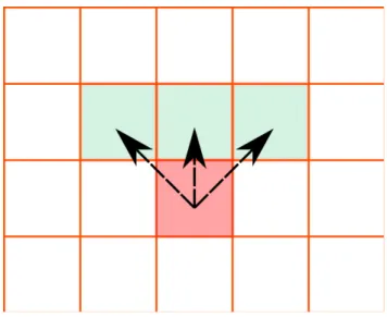
We define the arcs in the graph needed to ensure the desired hanging and footwall slopes and the minimum width requirement. Thanks to the adopted cylindrical system, these two constraints can be split and considered separately.
Figure 3.2 Block model under cylindrical coordinates a), and typical arcs in vertical section in proposed method b).
Stope wall angle constraints
Consider a vertical section of the model passing by the raise center line. To mine block A, a series of neighboring blocks must also be mined to guarantee the required footwall and han-ging wall slopes, and to account for the needed open space in front of the block (towards the raise, see Fig. 3.2 b). The number of links vertically upward or downward depends on the slope constraints and the discretization parameters ratio ∆z/∆r. For example, with ∆z/∆r = 1 one link upward ensures a hanging wall slope of 45o, two links upwards, an hanging wall slope
of 63.4o. Conversely, to ensure an hanging wall of 55o with a single vertical link, then the
∆z/∆r ratio must be set to 1.43. Where the slope angles required for stability vary spatially (due for example to variations in geology or stress conditions), it would be necessary to iden-tify locally homogeneous zones having approximately the same slope constraints. In an area with short scale variations of the slope constraints, it would be prudent to adopt the largest slope angles to avoid any collapse of the stope.
Stope width constraint
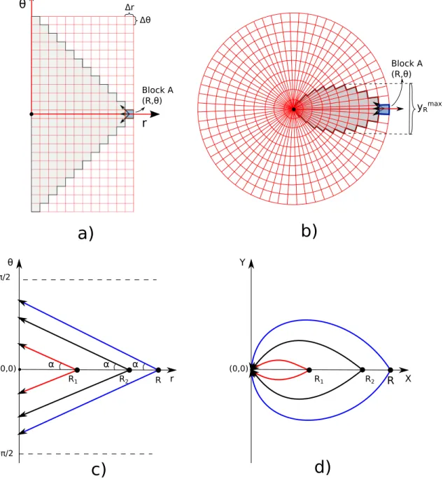
Consider now a horizontal plane in the cylindrical coordinates system having discretiza-tion ∆r and ∆θ. To move a block to the raise, enough open space in front of the block is required, so that the rock swelling after blasting does not impede the flow. This precedence relation suggests that a block should not be linked only to its immediate radial neighbor, but also laterally to its diagonal neighbors toward the raise (see Fig. 3.3 a). It is always possible to select the ratio ∆θ/∆r such that only three links are required in the horizontal plane toward the raise to meet the stope width requirement (see Fig. 3.3 b).
The links in the horizontal plane, propagated from block to block, eventually reach the raise center line (where r=0 in Fig. 3.3 a). In the Cartesian coordinates, it defines an envelope as shown in Fig. 3.3 b) and d). The maximum width of this envelope depends on the ratio K = ∆θ/∆r, and the radial distance R from block A to the raise center line. The width of the envelope for block A at any intermediate distance r along the line joining block A to the center line is :
yR(r) = 2rsin(θ)
= 2rsin(∆θ
∆r· (R − r))
= 2rsin(K · (R − r)) (3.5)
where K = ∆θ∆r and θ = K(R − r). The maximum width of the envelope yRmax can be calculated numerically using Eq. 3.5. The ymax
R depends on R and K. This formula conveys
the appealing idea that, to mine a block, the width of the open space needed increases with the block distance to the raise (see Fig. 3.3 c-d). R can be seen as a design parameter set by the mining engineer. It is the maximum radial distance a block may have from the current raise. Once this parameter is set, the second design parameter is the maximum width ymax
R
of the envelope required for this most extreme block to flow to the raise. Having R and yRmax, one may fix K by virtue of Eq. 3.5. Fig. 3.4 gives the K values as a function of ’Reference Distance to Raise’ (R) and ’Stope Width Parameter’ (ymaxR ).
3.3.6 Algorithm
The optimization algorithm comprises two main parts. The first part, the stope optimizer, is the core of our approach. It consists, for a specified raise location and height, to optimize
Δr Δθ Block A (R,θ) Block A (R,θ)
a)
b)
yRmax π/2 -π/2 θ (0,0) r α Y (0,0) X α α R1 R Rc)
d)
R2 R1 R2 θ rFigure 3.3 Horizontal plane showing blocks and links defined in the cylindrical system a) and corresponding blocks and links in the Cartesian system b). Shaded blocks represents blocks to be removed to get access to block A. Trace of the envelopes defined by the lateral links (function of K and R) in the cylindrical system c) as they appear in the Cartesian system d). Envelopes are computed with Eq. 3.5.
0.1 0.2 0.3 0.4 0.4 0.5 0.5 0.6 0.6 0.7 0.7 0.8 0.8 0.9 0.9 1 1 1.2 1.2 1.5 1.5 2 2 3 3 4 5 6 8 10 12
Reference distance to raise (m)
Stope width parameter (m)
10 15 20 25 30 35 40 1 2 3 4 5 6 7 8 9 10 Figure 3.4 K = ∆θ
∆r parameter (degree/m) as a function of control parameters R (reference
distance to raise) and ymax
R stope width parameter. For example, a block at 20 m from the
raise with a maximum width of 6 m necessitates a discretization approximately K = 1.7 degree/m with a single lateral link on both sides of the radial link as in Fig. 3.3.
the stope value given the chosen design parameters (R and ymax
R ) and slope constraints. The
stope optimizer involves the following steps :
1. Construct economic block model in cylindrical coordinates with current raise location and height as reference axis ;
2. Build the graph with vertical arcs for footwall and hanging wall slope constraints (see subsection 3.3.5) and horizontal arcs for width constraints (see subsection 3.3.5) ; all these arcs receive infinite capacities (following Picard (1976)) ;
3. Add the source and sink nodes to the graph. Positive nodes are linked to the source with capacities equal to their value and negative nodes are linked to the sink with capacities equal to their absolute value ;
4. Solve the maximum flow problem using an efficient algorithm. The sum of the residual capacities on the arcs linking the source to the positive nodes is the current stope value. This stope is conditionally optimal to the raise location and height.
In the second part one searches the best raise location and height using as objective func-tion the stope value found with the stope optimizer. This is done here by global optimizafunc-tion on the raise location and height parameters using the pattern search method (Audet and Dennis, 2003)).
After the overall optimal stope is found, we convert it to the Cartesian system. For this, each point of a fine Cartesian grid (here 1 m x 1 m x 1 m) is included in the final stope, or not, according to the state (in or out) of the closest cylindrical block centroid. The strategy of using the block centroid instead of the entire cylindrical block enables to smooth out the jigsaw profile that would otherwise appear due to the irregular shape of blocks defined in the cylindrical system (see Fig. 3.3. The final reported stope value (e.g. in Table 3.2) is computed from the points of the Cartesian grid identified to be in the stope. In our tests, the stope values computed in the Cartesian system were generally slightly smaller than the stope values computed in the cylindrical system.
3.3.7 Floating stope technique
The floating stope technique (Alford, 1996) is used for comparison with our method. The floating stope is implemented in some commercial softwares, such as Datamine and Vulcan. The user defines an elementary volume corresponding to the smallest volume justifying to create a stope. The elementary volume is moved over the entire block model and the profit
obtained in the volume at each location is computed. For each block of the model, the method notes also the location of the elementary volume which shows the largest profit among all the elementary volumes that include the block. A minimal envelope is obtained by the union of the elementary volumes with largest (positive) profits for each block. A maximal envelope is obtained by the union of all elementary volumes showing positive profit. The two envelopes provide a guide for the engineer to create a realistic stope which will normally lie somewhere between the minimal and maximal envelopes. In this method the engineer is obliged to incor-porate wall slope constraints manually. Comparison of the profits obtained with our method to the profits obtained with minimal and maximal envelopes is interesting, keeping in mind that our approach is the only one that ensures the satisfaction of slope constraints.
3.4 Results
To test the performance of the proposed algorithm, four different models, three synthetic and one real ore body, are used as input for the optimizer. The three synthetic cases are used to illustrate and help understanding the behavior of the proposed algorithm on perfectly known simple bodies. They are not aimed to represent real deposits. The shapes of synthetic ore bodies are kept simple so as to allow direct visual inspection of the feasibility and opti-mality of the stope. In those scenarios, the geotechnical constraints are given in Table 3.1. The discretization used for all cases was dr = dz = 1 m, and dθ computed with Eq. 3.5 (see Table 3.1). The floating stope method is also applied for comparison on the same cases with an elementary volume of 6 m × 6 m × 15 m that sweeps the same Cartesian grid as the one used to provide the optimized stope profit. The optimal stope values, missed ore values and waste included, for the different test cases, are presented in Table 3.2.
3.4.1 Test on synthetic ore block models
In the first scenario, a cross shape ore deposit is created (Fig. 3.5 a). The orebody is 20 m × 21 m × 25 m. The economic values of ore and waste blocks are set to 153$/t, and -23$/t respectively. The optimal stope is expected to include all the ore blocks, because the economic values of ores are high enough to pay for a large quantity of waste. Results are shown in Fig. 3.5 c) and d). The stope value is 868 k$. As expected, most of the ore blocks are taken into the stope together with the minimal amount of waste required to meet the hanging wall and footwall slope design.
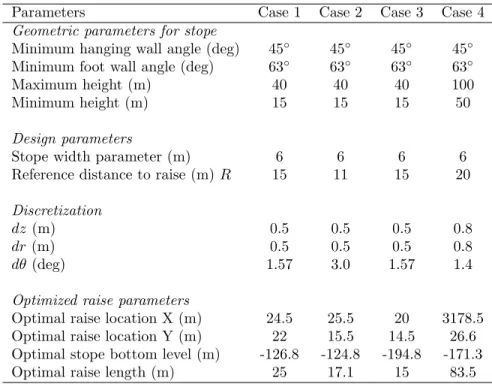
Tableau 3.1 Geometric and design parameters, discretization, and optimized raise parameters.
Parameters Case 1 Case 2 Case 3 Case 4
Geometric parameters for stope
Minimum hanging wall angle (deg) 45◦ 45◦ 45◦ 45◦ Minimum foot wall angle (deg) 63◦ 63◦ 63◦ 63◦
Maximum height (m) 40 40 40 100
Minimum height (m) 15 15 15 50
Design parameters
Stope width parameter (m) 6 6 6 6
Reference distance to raise (m) R 15 11 15 20
Discretization
dz (m) 0.5 0.5 0.5 0.8
dr (m) 0.5 0.5 0.5 0.8
dθ (deg) 1.57 3.0 1.57 1.4
Optimized raise parameters
Optimal raise location X (m) 24.5 25.5 20 3178.5
Optimal raise location Y (m) 22 15.5 14.5 26.6
Optimal stope bottom level (m) -126.8 -124.8 -194.8 -171.3
Optimal raise length (m) 25 17.1 15 83.5
Tableau 3.2 Economical evaluation of the case studies.
Cases Methods Stope profit
(k $) Missed ore value (k $) Waste value in stope (k $) Dilution volume rate1 Case 1 Network flow 868 2 -38.8 22.2% Floating stope(in)2 846 0 -62.3 31.3% Floating stope(out)3 436 0 -472.7 77.6% Case 2 Network flow 89 3 -22.1 56.9% Floating stope(in) 80 0 -34.4 66.7% Floating stope(out) -87 0 -201.3 92.1% Case 3 Network flow 442 0 -17.2 19.9% Floating stope(in) 424 0 -34.5 33.3% Floating stope(out) 153 0 -305.6 81.6% Case 4 Network flow 507 8 -2.6 3.3% Floating stope(in) 509 0 -8.3 8.1% Floating stope(out) 332 0 -185.9 41.0%
1Dilution volume rate = Volume of waste in stope / Volume of stope 2Float stope(in) : inner envelope created by floating stope method 3Float stope(out) : outer envelope created by floating stope method
Figure 3.5 Case 1, simulated ore model and stope by network flow method : a) 3D-view of the orebody, b) yz vertical section of the orebody at x=25, c) 3D view of the optimized stope, d) yz vertical section of the optimized stope at x=25 showing ore in stope (blue), waste in stope (red), and ore out of stope (green). Design parameters as given in Table 3.1