Publisher’s version / Version de l'éditeur:
Vous avez des questions? Nous pouvons vous aider. Pour communiquer directement avec un auteur, consultez la première page de la revue dans laquelle son article a été publié afin de trouver ses coordonnées. Si vous n’arrivez Questions? Contact the NRC Publications Archive team at
[email protected]. If you wish to email the authors directly, please see the first page of the publication for their contact information.
https://publications-cnrc.canada.ca/fra/droits
L’accès à ce site Web et l’utilisation de son contenu sont assujettis aux conditions présentées dans le site LISEZ CES CONDITIONS ATTENTIVEMENT AVANT D’UTILISER CE SITE WEB.
Technical Report; no. TR-2004-08, 2004
READ THESE TERMS AND CONDITIONS CAREFULLY BEFORE USING THIS WEBSITE.
https://nrc-publications.canada.ca/eng/copyright
NRC Publications Archive Record / Notice des Archives des publications du CNRC : https://nrc-publications.canada.ca/eng/view/object/?id=27263a13-4848-4711-89bc-017214ffb6dd https://publications-cnrc.canada.ca/fra/voir/objet/?id=27263a13-4848-4711-89bc-017214ffb6dd
Archives des publications du CNRC
For the publisher’s version, please access the DOI link below./ Pour consulter la version de l’éditeur, utilisez le lien DOI ci-dessous.
https://doi.org/10.4224/8895413
Access and use of this website and the material on it are subject to the Terms and Conditions set forth at CFD Code Evaluation
Institute for Ocean Institut des technologies Technology océaniques
CFD CODE EVALUATION
TR-2004-08 Eric Thornhill June 2004REPORT NUMBER
TR-2004-08
NRC REPORT NUMBER DATE
June 2004
REPORT SECURITY CLASSIFICATION
Unclassified DISTRIBUTION Unlimited TITLE CFD CODE EVALUATION AUTHOR(S) Eric Thornhill
CORPORATE AUTHOR(S)/PERFORMING AGENCY(S)
Institute for Ocean Technology, Memorial University of Newfoundland
PUBLICATION
SPONSORING AGENCY(S)
Institute for Ocean Technology, Memorial University of Newfoundland, Oceanic Consulting Corp.
IMD PROJECT NUMBER
42_2020_26
NRC FILE NUMBER
KEY WORDS
CFD, resistance, AUV, FLUENT, CFX, COMET
PAGES v, 32, App. A FIGS. 45 TABLES 7 SUMMARY
Report on an evaluation of three commercial CFD codes: FLUENT, CFX, COMET. The evaluation was based on usability, cost, technical support, and capabilities and other factors.
ADDRESS National Research Council Institute for Ocean Technology Arctic Avenue, P. O. Box 12093 St. John's, NL A1B 3T5
TABLE OF CONTENTS List of Tables ... iv List of Figures ... iv 1.0 INTRODUCTION ... 1 1.1 Background ...1 2.0 C-SCOUT SIMULATIONS ... 4 2.1 C-Scout Particulars...4 2.2 Experimental Results ...5
2.3 Fluent Simulations: 2d Laminar ...8
2.4 Grid Dependence Study ...9
2.4.1 Steady simulations ... 9
2.4.2 2D Transient simulations... 14
2.5 Comet Simulations: 2d Laminar...17
2.6 Fluent Simulations: 3d Laminar ...22
2.7 Comet Simulations: 3d Laminar...23
2.8 Fluent & Comet Simulations: 2d Turbulent (K - ε)...26
2.9 Fluent Simulations: 2d Axi-Symmetric Turbulent (K - ε)...28
2.10 Fluent Simulations: 3d Turbulent (K - ε)...28
2.11 Comet Simulations: 3d Turbulent (K - ε)...29
3.0 EVALUATION SUMMARY ... 30 3.1 CFX ...30 3.2 Comet ...30 3.3 Fluent...31 3.4 Conclusions / Recommendations ...31 Appendix A
LIST OF TABLES
Page
Table 1: C-SCOUT Experimental Resistance Results ... 7
Table 2: C-SCOUT 2D Grid Dimensions... 10
Table 3: C-SCOUT 2D Grid Dimensions... 12
Table 4: C-SCOUT 2D Grid Dimensions... 13
Table 5: C-SCOUT 2D Grid Dimensions... 14
Table 6: FLUENT & COMET BL Grid and y+ Values ... 27
Table 7: FLUENT BL Grid and y+ Values ... 29
LIST OF FIGURES Page Figure 1: C-SCOUT Configurations ... 4
Figure 2: Experimental Setup ... 5
Figure 3: Dimension of OERC Towing Tank ... 6
Figure 4: C-SCOUT Experimental Resistance Results... 7
Figure 5: Perimeter for 2D C-SCOUT Shape... 9
Figure 6: Surface Area for 3D C-SCOUT Shape... 9
Figure 7: 2D CFD Results: Coarse Grids ... 10
Figure 8: 2D CFD Results: Fine Grids ... 11
Figure 9: 2D CFD Results: Fine Grids with Boundary Layer Inflation... 12
Figure 10: Grids With and Without Symmetry Planes ... 13
Figure 11: Drag History: Grid2 – 2.0 m/s ... 15
Figure 12: Drag History Clip: Grid2 – 2.0 m/s ... 15
Figure 13: Drag History: Grid2_nbl – 2.0 m/s... 16
Figure 14: Drag History Clip: Grid2 – 2.0 m/s ... 16
Figure 15: Steady vs. Transient Results ... 17
Figure 16: FLUENT 2D Grid & COMET 2D Grid ... 18
Figure 17: Steady Laminar Simulations: Fine Grid, No Boundary Layer Grid 18 Figure 18: COMET Simulations: 2D, Laminar, Pseudo-Transient ... 19
Figure 19: COMET Simulations: 2D Laminar, No Boundary Layer Grid ... 20
Figure 20: Drag History: COMET 2D Laminar, No Symmetry Planes, 2m/s. 21 Figure 21: Drag History Clip ... 21
Figure 22: Quadrant 3D Domain... 22
Figure 23: Half 3D Domain ... 22
Figure 24: FLUENT 3D Laminar Results ... 23
Figure 25: 3D Laminar Half Domain: FLUENT & COMET Results ... 25
Figure 26: COMET 3D Laminar Results ... 25
Figure 27: FLUENT: 2D, k-e, BL = 0.01, 1.3, 7 ... 26
LIST OF FIGURES
Page Figure 29: FLUENT 2D Axi-Symmetric Transient Turbulent Results... 28 Figure 30: FLUENT 3D Transient k-e Quad Domain, proper y+ ... 29 Figure 32: grid1 ... A-2 Figure 33: grid1_bl2 ... A-2 Figure 34: grid1_nbl... A-3 Figure 35: grid1_nbl_r1 ... A-3 Figure 36: grid1_nbl_r2 ... A-4 Figure 37: grid1_r1 ... A-4 Figure 38: grid1_r2 ... A-5 Figure 39: grid1_r2b ... A-5 Figure 40: grid1h_nbl ... A-6 Figure 41: grid1h_nbl_r1 ... A-6 Figure 42: grid1h_nbl_r2 ... A-7 Figure 43: grid1h_nbl_r3 ... A-7 Figure 44: grid1h_nbl_rt ... A-8 Figure 45: grid2_nbl... A-8
1.0 INTRODUCTION
Computational fluid dynamics is a rapidly developing field in the marine industry. Numerical simulations of various flow processes allow detailed descriptions of pressure and velocity fields. Although IOT had made efforts to improve its capabilities to perform numerical simulations, there are still areas that need development.
Due to the fast paced nature of current CFD advancement, competitive software development for anything other than specific niche type problems is beyond our resources. The use of general-purpose commercial CFD codes is therefore the best option. We can benefit from ongoing code development and technical support from the code provider while focusing efforts on using and tailoring the software to solve
problems related to our own research/academic/commercial interests. Commercial CFD software does, however, require a substantial financial commitment (in the range of $20k – $40k per annum for licensing; dedicated computer hardware would also be necessary) and with several companies to choose from; the choice of which code will best meet our needs is not clear.
The purpose of this project was to evaluate three commercial CFD software packages in order to determine which would best be suited to marine and ocean technology related problems. Both Memorial University and Oceanic Consulting Corp. have an interest in CFD codes for their own research/academic/commercial interests that are generally closely aligned with those of IOT. As such, this was a collaborative project with each party contributing resources or knowledge.
1.1 Background
There are several competing commercial CFD software codes available in the market today. When deciding on which codes would be appropriate for the evaluation, several factors were considered. These include the code’s ability to handle; unstructured hybrid grids, adaptation, free surfaces, transient calculations, different turbulence models, and parallel processing. The codes that had all of the key elements were: FLUENT, CFX, COMET, and STARCD. Both COMET and STARCD were from the same vendor (ADAPCO) who recommended COMET as it has been used the most for marine related CFD problems.
FLUENT had been in use at Memorial University since 1999, and Oceanic had been using CFX since about 2000. Both codes had similar attributes but neither was clearly superior for hydrodynamics applications. An ADAPCO representative came to IOT in 2002 and gave a presentation on COMET capabilities, many of which were ship related. It was understood that if MUN, IOT, and Oceanic were all using the same CFD code, then sharing of resources, expertise, and techniques would benefit all concerned. The CFD evaluation project was then initiated to determine which code should be adopted by the community.
As commercial licenses were prohibitively expensive for this evaluation, educational licenses at MUN were used. The FLUENT license was continued, and a one-year
educational license for COMET was purchased, partially funded by IOT. An educational license for CFX was also purchased for MUN by Oceanic (in addition to the full
commercial CFX license already in use by Oceanic).
This evaluation project originally consisted of three phases:
Phase I. Simulations of C-SCOUT will provide an evaluation of the fully
submerged external flow (i.e. no free surface) capabilities of the various codes.
Phase II. Model 5415 (naval combatant surface ship) will be used to evaluate the free surface modeling capabilities of the test codes. Some work has already been conducted by Oceanic on this hull using CFX that will be made available. Similar cases will be run on both FLUENT and COMET for this project.
Phase III. P4119 marine propeller will be used to evaluate the codes’ ability to predict marine propulsor dynamics. It is also being used as the test case for the PROPELLA code currently under development at IOT.
Due to numerous unforeseen difficulties, only the first phase was attempted. Fortunately, enough work with the codes was achieved for the primary goal of the project to be realized; to determine which commercial CFD code best fits the needs of IOT/Oceanic/ MUN.
For reference purposes, a few of the significant problems that delayed or prevented progress on the projects other phases are listed here:
• There were delays in receiving and then setting up COMET both at MUN and IOT including several minor installation problems that took considerable time to overcome.
• COMET technical support was slow in responding to questions and often did not give full or clear explanations leading to further questions and hence delays in progress.
• Oceanic let its commercial CFX license lapse, which meant that only a single license (educational) at MUN was available for the evaluation project. This license was being used extensively by a graduate student (on a project for which the license was
originally acquired) making CFX access sporadic.
• The COMET user interface was considerably less sophisticated than its claims and price had suggested. Learning to use the software was slow and frustrating. Formal COMET training had been offered several times, but budget restrictions at IOT prevented this option until the 11th month of the one-year license. By that time most of the rudimentary usage of the program had been mastered. The training did, however, highlight potential problems with COMET when more advanced or problem-specific queries were met with uncertain responses.
• The FLUENT software at MUN was running on an older alpha Unix box (‘eddy’) that was slow when compared with current PC’s. Eddy was also not dedicated to
FLUENT usage which further slowed its processing when running multiple jobs.
• ‘Eddy’ was only accessible through computers in the graduate student computer lab. Often times this lab was full, delaying work with the code until a free computer became available.
• FLUENT discontinued support for alphas in 2001. As there was no other computer available, the last supported version for alphas remained on eddy and was therefore not kept current with upgrades.
• IOT along with MUN engineering contributed to a FLUENT research license purchased by the MUN physics faculty and run on computers in the Advanced Computation & Visualization Centre (CVC). The goal for the project being that the CVC hardware run larger and more complex cases than could be handled by eddy. However, the extensive usage by physics and chemistry faculty ultimately made FLUENT inaccessible.
• The graduate student working on this project was only part-time and between a full time job, courses, and learning the software, was not able to contribute sizable amounts of time to simulations for the project. This coupled with limited access to CFX meant that simulation comparisons presented in this report are only for FLUENT and COMET. Comments made about CFX were therefore drawn from previous experience with the code on other projects.
The causes of delays were generally due to problems with access; access to training and/or technical support, access to proper hardware, access to licenses, etc. One of the lessons learned from these experiences was that certain dedicated resources are necessary to maximize the usage of a CFD license. These include; appropriate computer hardware, money for formal training courses, and time for personnel to develop expertise with the code.
This report presents the results from the project that focused on the prediction of
resistance of C-SCOUT, a fully submerged body (i.e. no free surface effects) traveling at steady-speed through calm water. Resistance curves were computed for 2D & 3D
simulations for the FLUENT and COMET for a variety of speeds, grids, and solver settings. These were then compared quantitatively and qualitatively to experimental results. The final chapter of the report outlines the perceived differences in the three codes followed by recommendations.
2.0 C-SCOUT SIMULATIONS 2.1 C-Scout Particulars
C-SCOUT is an autonomous underwater vehicle (AUV) prototype currently in development at IOT and MUN. Based on a modular design strategy, the streamlined body-of-revolution hull of C-SCOUT can be extended in length to include various additional sections, such as bow & stern thruster combinations, and supplementary instrumentation sets. Three primary configurations of the vessel planned and shown below in
.
Length = 2.7m, Diameter = 0.4m 1. Nose Module
2. Releasable Ballast Module 3. Power & Computer Module 4. Fin Module
5. Tail Module
Length = 3.3m, Diameter = 0.4m 1. Nose Module
2. Fin & Releasable Ballast Module 3. Through-body Thruster Module 4. Power & Computer Module 5. Through-body Thruster Module 6. Fin Module
7. Tail Module
Length = 4m, Diameter = 0.4m 1. Nose Module
2. Payload Module
3. Fin & Releasable Ballast Module 4. Through-body Thruster Module 5. Power & Computer Module 6. Through-body Thruster Module 7. Fin Module
8. Tail Module
Figure 1: C-SCOUT Configurations
The CFD study focused on the first configuration and which, depending on operational requirements, was expected to have a maximum forward speed of 3.0 m/s.
2.2 Experimental Results
Physical model tests of the full-size C-SCOUT hull were conducted at the MUN towing tank. The model was mounted to the test frame as shown in Figure 2 for the bare hull model (configuration I: 2.7m in length) without any appendages. The results from the tests are shown in Figure 6 and Table 8.
Figure 3: Dimension of OERC Towing Tank
It was noted during these tests that above 2 m/s, a significant amount of surface waves were being produced. As a result, a significant amount of wavemaking resistance appears in the data at speeds greater than 2 m/s. Ideally, the vehicle would have been deeply submerged, but the MUN Towing Tank did not have the required depth to eliminate free surface effects at all speeds.
Tests in the astern direction were conducted to a maximum speed of 2 m/s only. This was the maximum speed of the MUN Towing Tank carriage in the astern direction.
0 20 40 60 80 100 120 140 160 180 0.0 0.5 1.0 1.5 2.0 2.5 3.0 3 Model Speed [m/s] Total Resi stance [N] .5 Forward Results Aftwards Results
Figure 4: C-SCOUT Experimental Resistance Results
Ahead Direction Astern Direction
Speed Resistance Speed Resistance [m/s] [N] [m/s] [N] 0.60 4.84 0.61 5.31 0.70 6.29 0.71 7.00 0.80 7.99 0.81 8.93 0.90 9.88 0.91 11.18 1.00 11.76 1.01 13.45 1.10 13.88 1.11 15.87 1.20 16.28 1.21 18.51 1.30 18.68 1.31 21.14 1.41 21.25 1.41 24.14 1.50 23.80 1.52 27.38 1.60 27.24 1.61 30.48 1.71 30.58 1.72 34.04 1.81 33.81 1.82 37.52 1.91 37.43 1.92 40.86 2.01 41.14 2.02 44.66 2.11 46.40 2.31 60.88 2.51 76.89 2.71 98.81 2.91 127.63 3.11 160.14
2.3 Fluent Simulations: 2d Laminar
The first phase of the CFD evaluation project was to perform simple 2D simulations on the bare hull of the C-SCOUT vessel. Although strictly speaking this was a 2D axi-symmetric case, the standard 2D solver was initially used due to difficulties in generating an appropriate mesh in COMET for comparing results. The domain geometry and mesh particulars are given in Appendix A.
Initial simulations evaluated the affects of various mesh densities and configurations along with the influence of various turbulence models using a steady-state solution method. The solution residuals (which show the progress of the iterative matrix solving procedure) for steady-state solutions showed that convergence was slow and often would level out or oscillate (e.g. continuity residuals would fluctuate between 0.002 and 0.004 where a value less than 0.001 was considered converged).
The geometry for the domain of a simple 2D resistance simulation is shown in Figure 31. Only half of the C-SCOUT bare hull cross-section was needed due to symmetry. A velocity inlet was located 2m ahead of the bow. The total length of the domain is 12m, with an outlet on the far right side. From the symmetry plane to the top of the domain was 2m. The top wall was specified as having zero shear stress (i.e. a free slip wall). A no-slip boundary condition was applied to the hull surfaces. The majority of the domain was meshed with unstructured triangular elements, except near the hull surfaces were a quadrilateral boundary layer grid was produced. Mesh spacing was also concentrated near the C-SCOUT surfaces.
A resistance curve was fit through a series of steady state simulations with varied the inlet velocities by computing the net force on the body in the x-direction. The 2D
resistance computed by FLUENT was that for a body the shape of the C-SCOUT hull per metre depth. To facilitate the comparison of the numerical data with the experimental data, the 2D surface area was “converted” to 3D surface area by dividing by the perimeter of the 2D body and multiplying by the surface area of the 3D body. Because the
C-SCOUT is actually a body of revolution, this approach is not strictly correct, but it did allow qualitative comparisons with the experimental data.
D 2 D 2 D 3 D 3 Fx Area Area Fx = ⋅ [1]
Area2D = Perimeter2D × unit depth [2]
where,
Fx3D is the x-direction force on a 3D C-SCOUT shape
Fx2D is the x-direction force on a 2D C-SCOUT shape (from CFD)
Area2D is the area of the 2D C-SCOUT shape
Area3D is the area of the 3D C-SCOUT shape (3.0991 m2) (see Figure 6)
Perimeter
Figure 5: Perimeter for 2D C-SCOUT Shape
Surface Area
Figure 6: Surface Area for 3D C-SCOUT Shape
2.4 Grid Dependence Study
2.4.1 Steady simulations
An important factor in any numerical study is the grid used to define the geometry and domain of the problem. The shape, size, and quality of the grid cells can have a direct affect on the results of the simulation: grid dependence. Ideally, a grid-independent solution is sought where changes or refinements to the grid do not result in significant changes to the calculated flow. Several grids were investigated for the C-SCOUT domain geometry (see Figure 31) for a steady-state laminar flow solution.
The first set of grids started from an initially ‘coarse’ base grid. This grid was an
unstructured triangular grid and did not include any boundary layer elements inflated off the hull surfaces. Three sets of refinements were then made to this grid. The first
refinement modified all cells within 0.15m of the hull surfaces with hanging node
adaptation (Coarse Grid R1). The second refinement further refined this grid, affecting all cells within 0.1m of the hull surfaces (Coarse Grid R2). A third grid was also tested which refined the entire domain of the initial base grid (Coarse Grid RT).
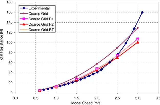
0 20 40 60 80 100 120 140 160 180 0.0 0.5 1.0 1.5 2.0 2.5 3.0 3.5 Model Speed [m/s] Total Resistance [N] Experimental Coarse Grid Coarse Grid R1 Coarse Grid R2 Coarse Grid RT
Figure 7: 2D CFD Results: Coarse Grids
The results show that the base coarse grid did not follow experimental results trend well. Improvement was seen after the first refinement and a smaller improvement was again seen after the second level of refinement. This shows that a grid-independent solution was not yet achieved. The ‘Coarse Grid RT’ results were nearly identical to the ‘Coarse Grid R1’ curve showing that refinement of cells outside of the 0.15m zone from the hull surfaces did not affect the resistance results.
Coarse Grid Coarse Grid R1 Coarse Grid R2 Coarse Grid RT
Bow 0.02 0.02 0.02 0.02 Midbody 0.04 bell 0.58 0.04 bell 0.58 0.04 bell 0.58 0.04 bell 0.58
Aft Taper 0.02 0.02 0.02 0.02
Aft End 0.02 0.02 0.02 0.02
Front Sym. 0.044 succ 1.03 0.044 succ 1.03 0.044 succ 1.03 0.044 succ 1.03 Aft Sym. 0.096 succ 0.973 0.096 succ 0.973 0.096 succ 0.973 0.096 succ 0.973
Inlet 0.2 0.2 0.2 0.2
Outflow 0.2 0.2 0.2 0.2
Top 0.2 0.2 0.2 0.2
Bound. Layer N/A N/A N/A N/A
Refinement N/A 0.15m 0.15m, 0.1m ALL
Total Cells 9113 12632 22178 36452
The next set of grids started from a base grid with approximately twice the resolution of the ‘coarse grid’. As before, the base ‘fine grid’ was tested. This grid was then refined to within 0.15m of the hull surfaces (Fine Grid R1). A third grid was used with a refinement on the Fine Grid R1 mesh on all elements within 0.1m of the hull surfaces (Fine Grid R2). 0 20 40 60 80 100 120 140 160 180 0.0 0.5 1.0 1.5 2.0 2.5 3.0 3.5 Model Speed [m/s] Total Resistance [N] Experimental Fine Grid Fine Grid R1 Fine Grid R2
Figure 8: 2D CFD Results: Fine Grids
The fine grid results showed good qualitative agreement with the experimental results. After one level of refinement there was negligible change (suggesting a grid-independent solution). The results from the second level of refinement differed significantly with high resistance values particularly at the higher speeds. A hump was also seen in the resistance curve that was not produced in any of the other simulations. This was clearly a grid-dependent phenomenon.
Fine Grid Fine Grid R1 Fine Grid R2
Bow 0.01 0.01 0.01 Midbody 0.02 bell 0.58 0.02 bell 0.58 0.02 bell 0.58
Aft Taper 0.01 0.01 0.01
Aft End 0.01 0.01 0.01
Front Sym. 0.05 succ 1.064 0.05 succ 1.064 0.05 succ 1.064 Aft Sym. 0.05 succ 0.983 0.05 succ 0.983 0.05 succ 0.983
Inlet 0.1 0.1 0.1
Outflow 0.1 0.1 0.1
Top 0.1 0.1 0.1
Bound. Layer N/A N/A N/A
Refinement N/A 0.15m 0.15m, 0.1m
Total Cells 33065 48635 91160
Table 10: C-SCOUT 2D Grid Dimensions
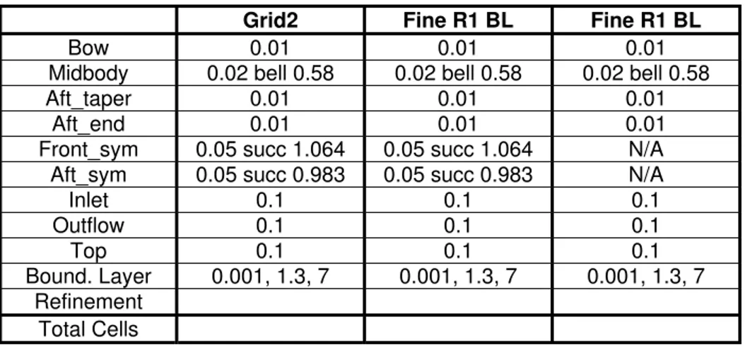
The next set of grids also included a boundary layer grid; a set of quadrilateral cells grown outwards from the hull surfaces. The same sets of refinement were performed and the results shown below.
0 20 40 60 80 100 120 140 160 180 0.0 0.5 1.0 1.5 2.0 2.5 3.0 3.5 Model Speed [m/s] Total Resistance [N] Experimental Fine BL Fine R1 BL Fine R2 BL
Fine BL Fine R1 BL Fine R1 BL
Bow 0.01 0.01 0.01 Midbody 0.02 bell 0.58 0.02 bell 0.58 0.02 bell 0.58
Aft_taper 0.01 0.01 0.01
Aft_end 0.01 0.01 0.01
Front_sym 0.05 succ 1.064 0.05 succ 1.064 N/A Aft_sym 0.05 succ 0.983 0.05 succ 0.983 N/A
Inlet 0.1 0.1 0.1 Outflow 0.1 0.1 0.1 Top 0.1 0.1 0.1 Bound. Layer 0.001, 1.3, 7 0.001, 1.3, 7 0.001, 1.3, 7 Refinement N/A 0.15 0.15, 0.1 Total Cells 32258 48881 97016
Table 11: C-SCOUT 2D Grid Dimensions
The results were all higher than the grids without boundary inflation, in some cases almost twice the values. There was some drag reduction after the first level of refinement. The second level of refinement led to only small changes.
Even the inclusion of the symmetry plane on the system seemed to have had significant results on the flow solution. In Figure 10 the results of simulations with and without a symmetry plane are shown for several grids. In the simulations with no symmetry plane, both the top and bottom of the C-SCOUT hull were meshed, resulting in a full 2D cross-section of the vessel and domain.
0 20 40 60 80 100 120 140 160 180 0.0 0.5 1.0 1.5 2.0 2.5 3.0 3.5 Model Speed [m/s] Total Resistance [N] Experimental Half Grid with BL Full Grid with BL Half Grid without BL Full Grid without BL
Grid2 Fine R1 BL Fine R1 BL
Bow 0.01 0.01 0.01 Midbody 0.02 bell 0.58 0.02 bell 0.58 0.02 bell 0.58
Aft_taper 0.01 0.01 0.01
Aft_end 0.01 0.01 0.01
Front_sym 0.05 succ 1.064 0.05 succ 1.064 N/A Aft_sym 0.05 succ 0.983 0.05 succ 0.983 N/A
Inlet 0.1 0.1 0.1 Outflow 0.1 0.1 0.1 Top 0.1 0.1 0.1 Bound. Layer 0.001, 1.3, 7 0.001, 1.3, 7 0.001, 1.3, 7 Refinement Total Cells
Table 12: C-SCOUT 2D Grid Dimensions
These results show that even though the geometry was symmetrical, different solutions were obtained depending on whether half or the entire domain was meshed.
2.4.2 2D Transient simulations
An observation made during many of the steady state simulations, was that the solution was not convergent. In most cases the residuals (particularly for continuity) approached the desired value of 0.001 and then oscillated. To investigate this, several transient simulations of the C-SCOUT hull were conducted. For these, the full 2D domain was used, with no symmetry planes. Both the fine grid and the fine grid with a boundary layer mesh were investigated. Simulations began with the domain initialized to the inlet
velocity. Timestep size was 0.1 seconds, and simulations ran for 1 minute. It was observed that all of the simulations showed oscillatory characteristics in drag (after the flow stabilized after the initial start-up behaviour).
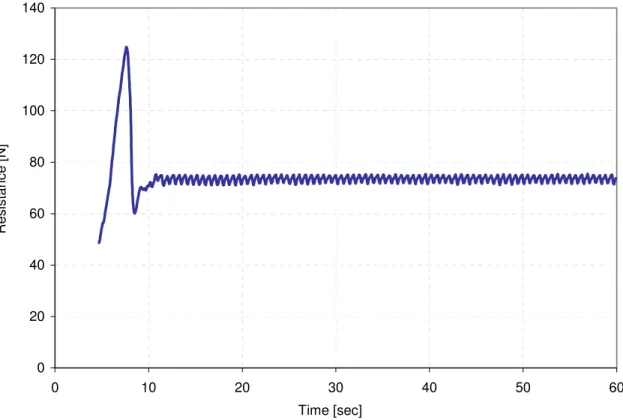
The results for the fine grid with boundary layer inflation are shown in Figure 11 and Figure 12. The oscillatory behaviour was not entirely regular as is shown in Figure 12. Average frequency was approximately 0.6 seconds and average amplitude was
approximately 3N.
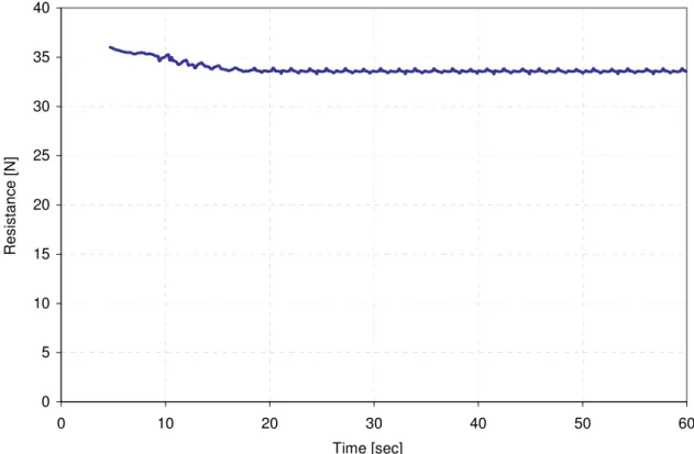
The fine grid without the boundary layer inflation showed considerably different results. Firstly, the mean net drag on the body was computed as nearly half that of the fine grid case with boundary layer inflation. The oscillation becomes more complex with
0 20 40 60 80 100 120 140 0 10 20 30 40 50 6 Time [sec] Resistance [N] 0
Figure 11: Drag History: Grid2 – 2.0 m/s
70 71 72 73 74 75 76 77 40 40.5 41 41.5 42 42.5 43 Time [sec] Resistance [N]
0 5 10 15 20 25 30 35 40 0 10 20 30 40 50 6 Time [sec] Resistance [N] 0
Figure 13: Drag History: Grid2_nbl – 2.0 m/s
33.2 33.3 33.4 33.5 33.6 33.7 33.8 33.9 34 40 41 42 43 44 45 46 47 48 49 50 Time [sec] Resistance [N]
The average results for drag for the transient simulation are shown below. Both grids showed differences between the steady and transient calculations.
0 20 40 60 80 100 120 140 160 180 0.0 0.5 1.0 1.5 2.0 2.5 3.0 3.5 Model Speed [m/s] Total Resistance [N] Experimental Fine with BL [Steady] Fine no BL [Steady] Fine with BL [transient] Fine no BL [transient]
Figure 15: Steady vs. Transient Results
2.5 Comet Simulations: 2d Laminar
This section discusses some of the results obtained using COMET for laminar 2D drag predictions of the C-SCOUT hull. Unlike FLUENT, COMET does not have a separate solver for 2D problems. Instead it solves a system that is one grid cell wide sandwiched between two symmetry planes. As a direct comparison between the FLUENT and
COMET solvers, the 2D grids produced by GAMBIT for the above FLUENT simulations were extruded one cell length to form appropriate grids for COMET and then imported using the NASTRAN file format.
Figure 16: FLUENT 2D Grid & COMET 2D Grid
Figure 17 shows the results of a comparison between predictions on a 2D grid in FLUENT, an extruded one cell deep 3D grid in FLUENT (semi-3D), and the extruded grid in COMET (COMET 2D). The results from the FLUENT simulations show that the 2D solver and a one cell deep 3D grid in the 3D solver produce nearly identical results. The COMET predictions with the same grid under predicted FLUENT results.
0 20 40 60 80 100 120 140 160 180 0.0 0.5 1.0 1.5 2.0 2.5 3.0 3.5 Model Speed [m/s] Total Resistance [N] Experimental Fluent 2D Fluent Semi-3D Comet 2D
Another difference between the FLUENT and COMET solvers was the mode used to achieve the steady-state solution. In FLUENT, there is either a steady state or a transient solver. The former neglects time-dependent components in the governing equations while the latter includes them. In COMET there is a third mode called “pseudo-transient”. This is used when there is difficulty achieving stable steady-state solutions. It retains the transient rate of change term, and takes relatively large time steps while only performing a single iteration per time step. It is not time accurate but this is not important for steady-state applications. All of the C-SCOUT simulations were found to be divergent with the steady-state solution mode in COMET. The pseudo-transient mode was therefore used. Figure 18 shows results from a similar comparison as that given for FLUENT in Figure 10. It compares results from 2D laminar (pseudo-transient) simulations for grids with and without a symmetry plane at C-SCOUT’s centerline, along with those with and without a boundary layer grid. There was generally less spread in the results compared with the FLUENT predictions; there was virtually no difference between the full and half domain results for the grid without boundary layer inflation. There was some difference between the full and half domain simulations with a boundary layer grid. Most notable was that the difference between the simulations with and without the boundary layer grid were significantly less than those produced by FLUENT.
0 20 40 60 80 100 120 140 160 180 0.0 0.5 1.0 1.5 2.0 2.5 3.0 3.5 Model Speed [m/s] Total Resistance [N] Experimental Half Grid, No BL Full Grid, No BL Half Grid, with BL Full Grid, with BL
Some transient mode simulations were also performed with these meshes in COMET and it was found that the average drag forces sometimes under-predicted those produced by the pseudo transient calculations. It was noted that COMET required a much smaller timestep for stability than did FLUENT (0.01s vs. 0.1s). This required that many more timesteps were necessary to see forces reach steady state. Figure 19 shows the results of the 2D laminar mesh with no boundary layer inflation for both the pseudo-transient and transient solutions methods.
0 20 40 60 80 100 120 140 160 180 0.0 0.5 1.0 1.5 2.0 2.5 3.0 3.5 Model Speed [m/s] Total Resistance [N] Experimental Pseudo Transient
Figure 19: COMET Simulations: 2D Laminar, No Boundary Layer Grid
A transient run of Grid2_nbl was performed but did not show the same sort of oscillating behaviour seen in the FLUENT transient simulations with the same grid. Instead, the force history seemed contained random noise as shown in Figure 20 and Figure 21.
0 5 10 15 20 25 30 35 40 0 2.5 5 7.5 10 12.5 15 17.5 20 22.5 Time [sec] Total Resistance [N]
Figure 20: Drag History: COMET 2D Laminar, No Symmetry Planes, 2m/s
33 33.1 33.2 33.3 33.4 33.5 33.6 33.7 33.8 10 11 12 13 14 15 16 17 18 19 20 Time [sec] Total Resistance [N]
2.6 Fluent Simulations: 3d Laminar
This section describes the results of 3D laminar simulations performed in FLUENT. Two domain types were explored: a quadrant and a half section. A full 3D domain was not investigated due to computational limitations. The quadrant and half domains were essentially the 2D domain sweep through 90 and 180 degrees respectively, with symmetry planes at the ends.
Symmetry Plane
Symmetry Plane
Figure 22: Quadrant 3D Domain
Symmetry Plane
Figure 23: Half 3D Domain
Figure 24 shows the results from the 3D laminar simulations. There was good agreement between results. Both the quadrant and half domains and transient and steady solutions gave similar results. However, these were all found to under predict the experimental results.
0 20 40 60 80 100 120 140 160 180 0.0 0.5 1.0 1.5 2.0 2.5 3.0 3.5 Model Speed [m/s] Total Resistance [N] Experimental Quad Steady Quad Transient Half Steady Half Transient
Figure 24: FLUENT 3D Laminar Results
2.7 Comet Simulations: 3d Laminar
A comparison of the 3D laminar results for the half domain grid generated by FLUENT (meshing program GAMBIT) by FLUENT and COMET is shown in Figure 25.
The 3D laminar results for COMET on the quadrant domain are shown below in Figure 26. In this figure, the grids were not the same as those used in FLUENT but were generated with the ADAPCO software PROAM. The domain size was the same as the FLUENT meshes, and the average mesh size was similar. The meshing topology was different than that employed by Gambit, a brief description is given in below. As with the FLUENT results, they were in good agreement with each other, but under predicted the experimental results. Also above approximately 2 m/s, the COMET results were slightly lower than the FLUENT results.
The COMET software has its own native meshing component, but it is very primitive and relies on text commands outlining locations of vertices and to connect them, in order, to form elements. Only rudimentary meshes can be created with this method, and with some difficulty. The PROAM software that is bundled with COMET is a modern fully
functional meshing program and can be used to generate practical meshes.
Though PROAM and GAMBIT share a similar function, they have two significantly different approaches. GAMBIT creates meshes from geometric volumes (ACIS solids) that are made up of ‘faces’ (surfaces and planes), which are in turn made from ‘edges’
(lines and curves) that are built from ‘vertices’ (points in space). One of the advantages of this approach is that CAD solids can be imported directly into GAMBIT and meshed. Due to the way they are defined, Boolean operations can be applied to the faces and volumes (e.g. a ship shape can be ‘subtracted’ from the water domain). A disadvantage is that all of the geometry of surfaces and curves must be ‘clean’ (i.e. no very short edges, overlaps, gaps, or loops) in order for a volume to be created and/or meshed. Difficulties in the geometry definition can lead to problems meshing, so time must be taken to ensure the a clean geometry.
PROAM does not require CAD solids; it instead brings in surfaces (IGES format) on which it then defines a surface mesh (the IGES file may have to be cleaned to remove some of the problems described above). From then on, only that surface mesh is used to define the geometry for later meshing processes, the IGES surfaces are no longer needed. As the surface mesh is simply a collection of triangles, there can be no problems with IGES formats on the volume meshing. PROAM can do standard tetrahedral and hybrid meshing (similar to GAMBIT) but also has a meshing approach called ‘trimmed cell’. A trimmed cell mesh starts with a Cartesian mesh block that aligns with, or slightly overlaps the maximum extents of the geometric domain. This mesh is composed of pure right-angled hexahedral elements. In the next step, the elements that overlap the surface meshes of the domain are ‘trimmed’ and elements that fall in void areas (like inside a ship) are removed. The result is a predominately hexahedral mesh, with some polyhedral elements near domain surfaces. The ability of COMET to handle arbitrary polyhedral elements is part of what makes this method useable. This method also comes with a technique that allows a boundary layer mesh (as was created with GAMBIT) around wall surfaces. This meshing technique has the potential to produce more efficient, and higher quality meshes than standard tetrahedral/hybrid meshing.
Although the trimmed cell technique worked well for the simple C-SCOUT geometry, when more complicated geometries were attempted (such as a planing hull with keel), problems emerged, particularly with the boundary layer meshing. COMET technical support was consulted about these difficulties, but did not have an answer.
Another disadvantage with the method, and PROAM in general, is that its not designed to create 2D meshes. The creation of 2D meshes requires that a full 3D mesh be created, all but one side deleted, and the remained side extruded to one cell deep (needless and time-consuming steps).
0 20 40 60 80 100 120 140 160 180 0.0 0.5 1.0 1.5 2.0 2.5 3.0 3.5 Model Speed [m/s] Total Resistance [N] Experimental
Half Domain (Fluent Grid) Half Domain (Proam Grid)
Figure 25: 3D Laminar Half Domain: FLUENT & COMET Results
0 20 40 60 80 100 120 140 160 180 0.0 0.5 1.0 1.5 2.0 2.5 3.0 3.5 Model Speed [m/s] Total Resistance [N] Experimental
Half Domain (Fluent Grid) Quad Domain
Half Domain
2.8 Fluent & Comet Simulations: 2d Turbulent (K - ε)
As the flow around C-SCOUT was mostly a turbulence flow (Re ~ 1x10⁶ to 8x10⁶), the effects of turbulence modeling were then explored in the numerical models.
The k-e turbulence model is a widely used eddy-viscosity based method of simulating the effects of near wall turbulence. There are special grid considerations near solid
boundaries when using this model that are related to the types of “wall functions” used to define the near wall boundary layer shape without the need of highly defined grid.
The FLUENT manual recommends that the fist cell is placed in the log-layer. The y+ value for the first cell should be 30 < y+ < 60 (closer to 30 is most desirable). It is also important to have at least a few cells inside the boundary layer. The COMET manual also gives recommendations for the y+ of the first cell in a boundary layer but with a slightly larger range 30 < y+ < 150.
In FLUENT the k-e turbulence model in 2D tended not to match the experimental results. Shown in Figure 27 are the results from a simulation investigating the effects of the initial and inlet values for k and e. The same mesh was used for each speed. Values of y+ in the first cell next to the hull ranged from 110 (1m/s) to 300 (3m/s).
0 20 40 60 80 100 120 140 160 180 0.0 0.5 1.0 1.5 2.0 2.5 3.0 3.5 Model Speed [m/s] Total Resistance [N] Experimental k=e=0.001 k=e=0.0005
Figure 27: FLUENT: 2D, k-e, BL = 0.01, 1.3, 7
The following figure has the results of 2D simulations for both FLUENT and COMET on the same grids. These were transient simulations1 and were run until the net drag reached
1
Steady simulations in Fluent and pseudo-transient simulations in Comet did not converge. Residuals would level off before convergence.
a constant level (results were not oscillatory). COMET took approximately 10 – 15 seconds of simulation time (with timesteps of ~0.01s) and FLUENT took from 20 – 30 seconds (with timesteps of ~0.1s). As the y+ values needed to be within a certain range for applicability of the turbulence model, the same grid could not be used for each speed. Shown in Table 13 are the boundary layer grid parameters (first layer thickness, growth factor, number of layers) as well as the approximate y+ values for a position on the mid-section of the hull surface. The results show that the COMET solver tended to under-predict the FLUENT solver, and that this trend increased with increased speed.
0 20 40 60 80 100 120 140 160 180 0.0 0.5 1.0 1.5 2.0 2.5 3.0 3.5 Model Speed [m/s] Total Resistance [N] Experimental FLUENT COMET
Figure 28: FLUENT & COMET 2D Transient k-e Results
Speed [m/s] BL Grid FLUENT y+ COMET y+ 1 0.0025, 1.1, 5 58 57 2 0.001, 1.3, 5 44 38 3 0.001, 1.3, 5 66 63
2.9 Fluent Simulations: 2d Axi-Symmetric Turbulent (K - ε)
The section revisits the same grids and turbulence parameters used for the FLUENT 2D simulations, but with the bottom symmetry boundary condition changed to an “axis” boundary condition. The solver was then run in 2D axi-symmetric mode. This method calculates the 2D representation of the C-SCOUT hull as a body of revolution.
As with the previous 2D results, different grids were needed at different speeds in order to achieve y+ values within the recommended range. The results of the simulations are shown below in Figure 29. These values, unlike the previous 2D results, can be compared directly with the experimental results. The trend was followed fairly well. It was noted during the experiments that significant wave-making could be seen above 2 m/s, so it was expected that the numerical results should be lower beyond this point.
0 20 40 60 80 100 120 140 160 180 0.0 0.5 1.0 1.5 2.0 2.5 3.0 3.5 Model Speed [m/s] Total Resistance [N] Experimental Fluent 2D Axi-Symmetric
Figure 29: FLUENT 2D Axi-Symmetric Transient Turbulent Results
It was not clear how to successfully run 2D axi-symmetric problems in COMET. The necessary grid differs than the standard 2D grid in that they entire domain must be wedge shaped and still one cell thick. Technical support was asked, but no response was given.
2.10 Fluent Simulations: 3d Turbulent (K - ε)
As with the 2D models for the k-e model, a certain y+ range must be met in the first cells of the boundary layer grid. The following figure has the results from that simulation for a 3D quadrant of the domain (with two symmetry planes). The results show good
0 20 40 60 80 100 120 140 160 180 0.0 0.5 1.0 1.5 2.0 2.5 3.0 3.5 Model Speed [m/s] Total Resistance [N] Experimental Fluent Quad
Figure 30: FLUENT 3D Transient k-e Quad Domain, proper y+
Speed BL Grid FLUENT
[m/s] y+
1 0.0025,1.1,5 50
2 0.001,1.3,5 35
3 0.001,1.3,5 55
Table 14: FLUENT BL Grid and y+ Values
2.11 Comet Simulations: 3d Turbulent (K - ε)
At the time of writing, there was difficulty in producing results for 3D in COMET. Coarse boundary layer grids produced under-predicted results, and when grids closer to the resolution of the FLUENT grids were generated, it wasn’t possible to obtain a
convergent solution. Even when set to transient mode the simulations would only run for a few timesteps and then diverge.
Also in cases with coarse grids where convergence was achieved, the size of the timestep used in the pseudo-transient mode had a significant effect on the results. Different
pseudo-transient timestep sizes gave convergent solutions with widely varying drag results. Technical assistance at ADAPCO was contacted but a solution had not yet been found.
3.0 EVALUATION SUMMARY
The goals of this project were to evaluate three commercial general-purpose CFD codes, FLUENT, CFX and COMET. Each of these codes has similar cost and functionality; they are all 3D RANS codes that can take unstructured hybrid meshes, can handle free
surfaces and employ several options for turbulence modeling.
The evaluation was based on the abilities of the codes to handle marine and ocean-technology related problems such as hydrodynamic resistance. Several test phases were planned, but as a consequence of multiple setbacks (outlined in the introduction), only basic C-SCOUT simulations were conducted with FLUENT and COMET. Previous work with CFX by Oceanic was used in description of that codes capabilities.
3.1 CFX
• Ran on Windows operating system.
• Good graphical user interface (GUI), usage of code was fairly intuitive.
• Tended to be more like a ‘black-box’ than the other two codes in that more detailed controls were hidden from the user (some of which could be accessed if instructed by technical support, but wasn’t contained in the manuals).
• Although had many of the same overall functionality as FLUENT, some useful features were noticeably absent (e.g. being able to adapt cells based on proximity to a wall boundary).
• Had no pure 2D capability, relied on 3D meshes that were 1-cell thick. There was no easy way to create this mesh with their meshing software.
• Solver was robust and efficient. Extension to parallel processors was straightforward.
• Had no ‘moving mesh’ capability for fluid/structure interaction problems
• Post-processor was excellent. Visualization of flow and creation of quality plots for reports was relatively simple.
• Technical support was found to be slow to respond and was not always as helpful as would be expected.
3.2 Comet
• Only ran on UNIX/LINUX operating system.
• Program commands were entered through a combination GUI and a command-line style text user interface (TUI). The GUI was dated and cumbersome to use.
Rotate/pan/zoom controls for the display were done with sliding bars as opposed to mouse control. This made many operations slow and tedious. Mouse controls for these display functions are standard for modern CFD and CAD software. The text commands were likewise cumbersome. Command names were cryptic and relied on a selection structure based on cell, face, and vertex numbers. This approach would be reasonable for structured meshes, but for an unstructured mesh the numbering scheme has little significance outside of the solver.
• Mesh was done with a separate program PROAM and compared with COMET this software was modern in its GUI and general look and feel.
• PROAM was a good meshing software tool with many features. It’s approach differed slightly from FLUENT and CFX with pros and cons.
• The solver was first compiled with the given case before it was run, making it fairly efficient.
• COMET also has no pure 2D capability. As with CFX it required a 3D mesh that was one cell thick. Creating this mesh in PROAM was not straightforward.
• Post-processing capabilities in COMET were lacking. It had only the most basic options and creating more complicated plots required in-depth knowledge of text commands.
• Technical help was slow in responding.
• This code is scheduled to be re-released to more closely match ADAPCO’s STARCD general purpose CFD software. It is unclear how this will affect the program or its current users.
3.3 Fluent
• Runs on both UNIX and Windows operating systems.
• Uses both a relatively easy to understand GUI or a command-line TUI. Both use a series of straightforward menus and submenus to reach desired commands.
• Meshing is done with a separate code GAMBIT. This is reasonably good meshing software. It can handle 2D as well as 3D meshes both structured and unstructured approaches. The reliance on ACIS ‘volumes’ means that some effort may go into the getting the initial geometry to a mesh-ready form.
• Properly setting up simulation controls requires some training. General user-friendliness is slightly behind CFX but well ahead of COMET.
• FLUENT has a larger user group than either COMET or CFX and has generally been ahead in terms of development of new features.
• Technical support has usually been prompt and helpful.
3.4 Conclusions / Recommendations
FLUENT came out the strongest of the three codes. It was relatively easy to use, had the most features and the best technical support. COMET, the most expensive code, was found to be overly cumbersome and dated, though the solver itself seemed efficient. The PROAM meshing software, which came with COMET, had a lot of potential with its ‘trimmed-cell’ technique, but boundary layer inflation (needed for resistance simulations) became problematic for anything other than simply geometries. CFX was not tested directly in this study but considerable use of this code has been done by Oceanic. They found that the software had strong points but had difficulties with free surface resistance simulations. They also found that the geometry preparation for CFX meshing was excessively time-consuming.
Memorial University currently has educational licenses for FLUENT in both the
engineering and physics & chemistry faculties. IOT’s usage of this code would facilitate collaborations and widen the local user-base and sharing of expertise with the software. OCEANIC has let their CFX license lapse and may consider acquiring FLUENT should the demand for numerical work increase.
Commercial CFD software is a considerable financial commitment ($23,500 USD/year for FLUENT) and would also require dedicated high-end computer hardware. Although the software could be used for commercial projects, it will take some time before new users become proficient and develop a good understanding of the codes strengths and weaknesses for different problem types. If the code were acquired, a formal training session for interested researchers would be recommended.
Figure 31: G
eometry
Figure 32: grid1
Figure 34: grid1_nbl
Figure 36: grid1_nbl_r2
Figure 38: grid1_r2
Figure 40: grid1h_nbl
Figure 42: grid1h_nbl_r2
Figure 44: grid1h_nbl_rt