HAL Id: hal-00542436
https://hal.archives-ouvertes.fr/hal-00542436
Submitted on 2 Dec 2010
HAL is a multi-disciplinary open access archive for the deposit and dissemination of sci-entific research documents, whether they are pub-lished or not. The documents may come from teaching and research institutions in France or abroad, or from public or private research centers.
L’archive ouverte pluridisciplinaire HAL, est destinée au dépôt et à la diffusion de documents scientifiques de niveau recherche, publiés ou non, émanant des établissements d’enseignement et de recherche français ou étrangers, des laboratoires publics ou privés.
Jean-Philippe Vidal, Sabine Moisan, J.B. Faure, Denis Dartus
To cite this version:
Jean-Philippe Vidal, Sabine Moisan, J.B. Faure, Denis Dartus. Towards a reasoned 1-D river model calibration. Journal of Hydroinformatics, IWA Publishing, 2005, 7 (2), p. 91 - p. 104. �hal-00542436�
Towards a Reasoned 1-D River Model Calibration
Jean-Philippe Vidal (corresponding author)
CEMAGREF1
Hydrology-Hydraulics Research Unit 3 bis quai Chauveau
CP 220 69 336 LYON CEDEX 09 FRANCE [email protected] Sabine Moisan INRIA2 Sophia-Antipolis Orion Project
2004 route des Lucioles BP 93 06 902 SOPHIA-ANTIPOLIS FRANCE [email protected] Jean-Baptiste Faure CEMAGREF
Hydrology-Hydraulics Research Unit 3 bis quai Chauveau
CP 220 69 336 LYON CEDEX 09 FRANCE [email protected] Denis Dartus IMFT Hydre Group
Allée du professeur Camille Soula 31 400 TOULOUSE
FRANCE
1 French National Institute for Agricultural and Environmental Engineering Research 2 French National Institute for Research in Computer Science and Control
Abstract
Model calibration remains a critical step in numerical modelling. After many attempts to automate this task in water-related domains, questions about the actual need for calibrating physics-based models are still open. This article proposes a framework for good model calibration practice for end-users of 1-D hydraulic
simulation codes. This framework includes a formalisation of objects used in 1-D river hydraulics along with a generic conceptual description of the model calibration process. It was implemented within a knowledge-based system integrating a simulation code and expert knowledge about model calibration. A prototype calibration support system was then built up with a specific simulation code solving subcritical unsteady flow equations for fixed-bed rivers. The framework for model calibration is composed of three independent levels related respectively to the generic task, to the application domain, and to the simulation code itself. The first two knowledge levels can thus easily be reused to build calibration support systems for other application domains, like 2-D hydrodynamics or physics-based rainfall-runoff modelling.
Keywords
Introduction
Good modelling practice has recently become a topical subject in water-related domains (Scholten et al., 2000; Cunge, 2003). Indeed, numerical models have become essential tools in these domains, from research purposes to engineering applications. Throughout several generations of hydraulic modelling (see Abbott et al. (1991)), simulation codes have been evolving from basic numerical solvers to efficient and user-friendly hydroinformatic tools. But in spite of efficiency improvement, their use for advanced purposes still requires expertise.
In particular, good achievement of calibration task depends on the skills of the modeller, as this task is based on heuristic rules. This article aims at defining a framework for a “good model calibration practice” – to quote Guinot and Gourbesville (2003) – in 1-D river hydraulics. This framework is planned to be the core of a knowledge-based system integrating numerical tools – simulation codes – and semantic expert knowledge about their operational use in a calibration context. Using this system, practitioners may thus be guided during model calibration by expert reasoning.
The definition of a calibration framework requires first to consider what is called model calibration in the numerical modelling context. The first part of the article thus proposes preliminary thoughts on this task, including terminology issues but also observations on the role of calibration in a modelling study. A second part introduces knowledge involved in model calibration and presents tools used for its formalisation. The two following parts show our proposal of a framework for good practice, throughout two aspects. On the one hand, a conceptual description of concepts involved in model calibration gives a static view of objects used during this task in 1-D hydraulics and of relations between them. Such a conceptual description is called an
ontology in the Artificial Intelligence domain. On the other hand, a dynamic view of the corresponding
process is detailed within a generic conceptual description of the activity. Finally, an application of the developed knowledge-based system with a specific simulation code is outlined, and conclusions are drawn.
About Model Calibration
Model Calibration in the Numerical Modelling Context
Numerical modelling covers many different application domains, and thus various scientific communities using specific definitions, especially of generic terms like model. Therefore, we propose to use in this article a modelling terminology based on the attempt first made by the SCS Technical Committee on Model
Credibility (Schlesinger et al., 1979) and extended by Refsgaard and Henriksen (2004).
The corresponding graph in Figure 1 is composed of four elements linked by dashed arrows: • Reality is a generic physical system.
• The behaviour of this system is analysed to get a conceptual model, which is constituted of governing equations.
• Programming converts this conceptual model into a computer program: the simulation code. • This code is then applied to a particular system by model set-up to get a numerical model of this
system. This numerical model can then simulate the behaviour of the system by predictive simulation.
Outer arrows refer to the procedures which evaluate the credibility of the processes described by inner arrows. Model calibration is thus defined as the procedure which assesses that a model is properly set-up and that it simulates well the selected system.
Examples in hydrodynamic modelling can easily be derived from these generic definitions. In the following, we consider that the physical system is a fixed-bed river reach, and the corresponding conceptual model is Saint-Venant equations. The simulation code may thus be one of the many available codes able to solve
these equations. The selected code may be used to produce a numerical model which is able to simulate open channel flow in this particular reach. All examples of this article are taken from subcritical unsteady flow modelling of a single river reach.
Role of Calibration in the Modelling Activity
The commonly used modelling activity is defined by a four-step framework: model set-up, model
calibration, model validation, and finally exploitation (Cunge, 2003). A detailed generic framework has been developed by van Waveren et al. (1999) in order to define the current good modelling practice in water-related domains. This framework presents calibration as an alternative to formal identification of parameters if this procedure is impossible because of the lack of sufficient gauged data.
This remark led us to wonder about the actual definition of “model calibration”. Refsgaard and Henriksen (2004) propose the following one: “the procedure of adjustment of parameter values of a model to reproduce the response of reality within the range of accuracy specified in the performance criteria.” Modellers are often encouraged by decision makers to respect this performance criteria and they may unfortunately force parameter values in that way, leading to models with poor predictive capacities (for relevant examples in river hydraulics, see Abbott et al. (2001)). For this reason, Cunge (2003) discusses the four-step paradigm and proposes a new one for deterministic – or “physics-based”, as specified by Hall (2004) – models without calibration stage.
In our approach, we consider that calibration, defined as the procedure assessing model set-up, is a necessary stage in the modelling process. Indeed, calibration does not come down to tune parameters, but it implies many different reasoning processes to properly deal with the available data and to get a – relatively – reliable model. We thus propose to provide practitioners with guidelines extracted from engineering experience in order to avoid unrealistic parameter adjustments.
End-users of hydraulic simulation codes currently perform parameter adjustment by one of the two main traditional ways:
• Trial-and-error. This subjective method is based on visual comparison of computed and observed values, and manual adjustment of parameters. The major advantage of trial-and-error is its reliability, depending obviously on the level of expertise and on knowledge of the modeller about the site.
• Automatic optimisation. In order to overcome subjectivity problems, automatic calibration methods may be applied. They rely on three main elements: an objective function that measures the discrepancy between observations and numerical results, an optimisation algorithm that adjusts parameters to reduce the value of the function, and a convergence criterion that tests its current value. This very kind of calibration has been widely used in hydraulics over the last thirty years (see for example Wormleaton and Karmegam (1984), Khatibi et al. (1997), Anastasiadou-Partheniou and Samuels (1998)). The major drawback of optimisation stands in the equifinality problem – as defined by Beven (1993) – which predicts that the same result might be achieved by different parameter sets. Thus, local minima of the objective function might not be identified by the algorithm and lead to unrealistic parameter values and consequently to models with poor predictive capacities.
Guidelines to provide to practitioners belong to a wider knowledge about model calibration. This knowledge, constituting the symbolic part of our framework, was formalised to be integrated into a knowledge-based system.
Methods for Knowledge Formalisation
In a generic approach, knowledge about model calibration may be classified into three types, following Chau et al. (2002):
• Descriptive knowledge is about entities necessary in the model calibration process. These entities may be representations of real objects – e.g., a discharge hydrograph or a simulation code – but also concepts, like data or parameter.
• Procedural knowledge deals with activities performed during the model calibration process. These activities may include generic procedures – e.g., model calibration – or more specific ones, like
initializing roughness parameter values.
• Reasoning knowledge is about the way of using descriptive and procedural knowledge to carry out model calibration. This third type of knowledge is expressed by production rules as defined in Artificial Intelligence:
IF conditions THEN actions
Descriptive knowledge was formalised by building ontologies gathering and linking all the concepts involved in model calibration. A workflow for model calibration formalises the second kind of knowledge. After a preliminary graphic representation of descriptive and operative knowledge, all three kinds of knowledge were transcribed using a knowledge description language. Tools used for these steps are presented below.
Graphic Representation
We used the Unified Modelling Language (UML) and its associated object-oriented graphical formalism (OMG, 2003) to represent descriptive and procedural knowledge. This formalism has become a standard in computer science and is widely used for describing software artefacts. It served us as a tool to specify our prototype calibration support system.
Concerning descriptive knowledge, UML class diagrams served us to formalise objects involved in the model calibration task. These diagrams allow to represent descriptive concepts – as classes in the object-oriented sense – linked together thanks to two kinds of relationships. Associations – shown as lines with optional arrows for simple relations, or with hollow diamond for a subpart relation called aggregation – formalise semantic relationship between two or more classes. Generalisation is a taxonomic relationship between a more generic element and a more specific element. This second kind of relations is shown as a solid-line path with a large hollow triangle at the end of the path where it meets the more general element.
Concerning procedural knowledge, we used UML activity diagrams to formalise subtasks of the model calibration task. Within this kind of diagrams, an action-state – representing here a subtask – is shown as a shape with straight top and bottom and with convex arcs on the two sides. These actions operate on objects, which are instances of classes predefined in UML class diagrams. Flow between actions and objects are shown by dashed arrows. Decisions are represented by diamonds with guard conditions. Concurrent transitions between action states (synchronisations or splitting) are represented by short heavy bars.
Use of a Knowledge Description Language
Knowledge description languages allow to formalise knowledge in a both readable and operational way. The YAKL language, developed at INRIA (Moisan, 2002), particularly suited our problem, since it has been
developed for the formalisation of knowledge about the skilled use and planning of codes – called program
supervision (Moisan, 2003). It had been previously applied to image processing programs (Thonnat et al.,
1999) and was slightly adapted for simulation codes (Vidal et al., 2003).
The YAKL language supports both object and rule-oriented descriptions. It allows to get a textual translation
of UML class and activity diagrams for both descriptive and procedural knowledge. Moreover, reasoning knowledge can also be easily taken into account thanks to rule-oriented descriptions. Knowledge is
An inference engine, developed in INRIA together with the YAKL language, serves us to put this formalised
knowledge into practice. The result is an interactive knowledge-based system which adds a layer of expert-user knowledge on top of the simulation code itself.
1-D River Model Calibration Concepts
The static side of our framework has been formalised throughout an ontology of model calibration domain. It gathers descriptive knowledge used during this task, and extracted from both our experience and
interviews of experts.
Generic Concepts in Operational Validation
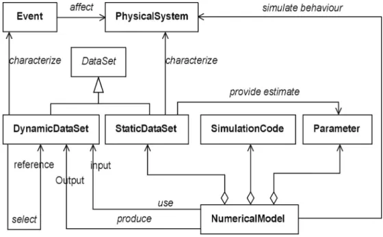
The first step in building an ontology is to define generic concepts that could be reused and specialised in several domains. The goal of operational validation is “to assure that the model compares well to perceived reality” (Knepell and Arangno, 1993). In other words, operational validation consists in comparing model results to reality and modifying the model if needed. What has to be noticed in this indirect definition is that it covers both calibration and validation stages of the current modelling paradigm. Thus, it could be easily related to the model proving stage detailed by Seed et al. (1993). Therefore, we decided to build up a generic formalisation of concepts from operational validation, which could be used in the particular case of model calibration. The resulting UML class diagram is presented in Figure 2.
The first formalisation step is the description of the physical part of the problem. The physical system to be modelled is linked with events affecting it. Following Amdisen (1994), we distinguish two types of data3:
static data are linked to the system itself and are supposed to be invariant. On the contrary, dynamic data
characterise events, by ways of measurement or computation.
For the modelling part of the problem, we define a numerical model as an aggregation of static data from the system, parameters and a simulation code. Simulation code and numerical model definitions are here in accordance with concepts from Figure 1. Static data provide estimates for parameter values. A numerical model uses dynamic data corresponding to some events as input data. Dynamic data produced by the simulation are called output data. These output data are then compared to reference data selected from the dynamic data set, to assess if the numerical model simulates correctly the behaviour of the system.
For instance, in river hydraulics, events may be floods affecting a given river reach. In our approach, static data include river reach topography and physical description. Thus, we do not take into account movable bed rivers and we assume that river topography is not to be adjusted during the calibration process. Dynamic data are constituted by hydraulic measurements or computational results related to a particular flood. A numerical model of the given reach is composed of static data detailed above, parameters – among them roughness parameters – and a simulation code solving flood propagation equations.
Data Specialisation for 1-D River Hydraulics
We then specialised generic concepts of static data and dynamic data in order to manipulate data specific to 1-D river hydraulics. Moreover, we focused on subcritical unsteady flow modelling.
3 Khatibi (2002) defines five types of data for different modelling problems, but the two classifications match well by
We first specialised dynamic data on the basis of their function in the calibration process, into input data,
reference data and simulation output data.
Then, we define input data – objects given to the model in order to run the simulation – as an aggregation of an upstream boundary condition, a downstream boundary condition, optionally a lateral boundary condition and a initial condition. An upstream boundary condition consists – in the case of subcritical unsteady flow modelling of a single river reach – of an input discharge hydrograph set at the upstream end of the river system modelled.
Simulation output data are computed results of the simulation run, whereas reference data are field data to compare these results with. For example, water-surface profiles may be part of the simulation output data, whereas floodmarks are attributes of reference data. Various natures of reference data may be used, some subjective, like witnesses, and some complex, like remote sensing data. At first, we restricted our analysis to the ones based on standard hydraulic measurements: floodmarks, water levels, and gaugings. Moreover, we did not take into account any imprecision or uncertainty on these values.
Formalisation of Concepts in 1-D River Hydraulics
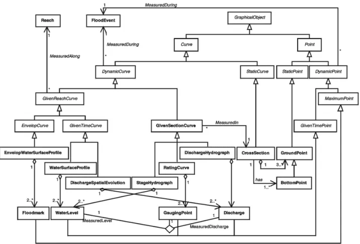
All 1-D river hydraulics data described in the previous section have been linked together in order to get a hierarchy of bidimensional graphs which can be easily manipulated in an object-oriented approach. The resulting hierarchy is shown in Figure 3.
The most generic concept of graphical object is first divided into curves and points subtypes. Points are then divided into dynamic and static points, depending if they are linked or not with a flood event. Ground points – and bottom points – inherit from static points. Water levels, gauging points, and discharges are dynamic
points measured – or computed – at a given time (GivenTimePoint in Figure 3). Floodmarks are dynamic points representing a maximum reached during a given duration (MaximumPoint).
Curves are in the same way divided into dynamic and static curves. Cross-sections are considered to be static curves. Rating curves, stage hydrographs and discharge hydrographs are dynamic curves measured in a cross-section (GivenSectionCurve in Figure 3) whereas water-surface profiles and discharge spatial
evolutions are dynamic curves measured along a reach (GivenReachCurve). Moreover, these two curves are measured or computed at a given time (GivenTimeCurve). Finally, envelop water-surface profiles are composed of maximum water levels (EnvelopCurve).
Proposed Workflow for Model Calibration
The dynamic side of our framework has been formalised throughout a workflow for model calibration as a generic task. This workflow was then used to define subtasks specialised for 1-D hydraulics.
Generic Workflow
Generic procedural knowledge about model calibration was formalised graphically in Figure 4. The
formalism used in this figure refers to the one described above in the presentation of UML activity diagrams.
This representation of generic procedural knowledge – constituting a paradigm for model calibration – was established on the basis of the formalisation of procedural knowledge used by experts to achieve this task. It is worth noting that this workflow contains implicitly the “sensitivity analysis” task. As a matter of fact,
performing manually a sensitivity analysis only requires to initialise parameters, to run a simulation and to start again, by applying appropriate reasoning rules.
We decomposed the model calibration task into six main generic subtasks. This kind of knowledge has been extracted from the few guidelines available (Cunge et al., 1980; Hill, 1998). The model calibration task aims at producing a well-calibrated model from an uncalibrated model and available data. Data allocation and parameter definition are executed in parallel within a global preprocessing task. Data allocation extracts two sets of data from the available data : inputs needed to run the simulation and references needed for the comparison with results from the simulation. Parameter determination aims at defining and initialising the model parameters. The model with initialised parameters is then used together with input data to produce outputs. These outputs are then compared with reference data. If no satisfactory agreement is found, model parameters are re-initialised or re-defined. Once an agreement has been reached – and if there is still available data – another couple of inputs/references is built up in order to draw other comparisons. Finally, the resulting model is evaluated considering the objectives of the calibration, and more generally of the modelling.
Each subtask of model calibration is described more precisely below. For each subtask, the functions that have been automated and implemented within the knowledge-based system are described. Examples of the formalisation of reasoning knowledge with the form of production rules written in the YAKL language are
also provided in the following paragraphs.
Description of Subtasks and Implemented Knowledge
Data Allocation
The first question one has to answer when calibrating a model is: “Which data will be used, and how?” The modeller has to choose among available data which of them will be used in the calibration process,
depending on the objective of the study. For example, a model intended to simulate flood propagation should be calibrated with measurements from past flood events, and not from low flow stage periods. The first step in data allocation is thus to select past events, and related dynamic data. These events should be as representative as possible of the variety of situations that the model should be able to reproduce. Another key point discussed by Khatibi (2001) is the minimum number of independent events to be used in order to get a satisfactory confidence in the calibrated model.
For each event, two sets should be constituted: input data, given to the code to run simulations, and reference data, used for comparison with simulation output data. There is sometimes no real choice for the number of field data is often very scarce. But this choice should always be made in agreement with the actual aim of the future calibrated model and with its “performance criteria”. During this task, the modeller may be encouraged to get hold of particular field data which prove to be indispensable to assess that the criteria will be reached or not.
An example of reasoning knowledge used during this subtask is provided by the following rule: if a
hydrograph was measured during the selected event in the upstream section of the modelled reach, it will be used as an upstream boundary condition for the simulation run.
This task should be repeated as many times as there are events from which the modeller can extract two coherent sets of data, in order to make use of field measurements in an optimal way.
Parameter Definition
The second important step in preprocessing is the definition of parameters. It aims at choosing which parameters will be tuned during the calibration process. In our approach, two kinds of physically-based parameters may be identified: localised parameters – e.g., discharge coefficient of a given hydraulic structure – and spatially and/or temporally distributed parameters – e.g., roughness coefficients. Whereas
localised parameters only require to be considered tunable or not, the definition of distributed parameters includes their number and position in the reach.
In river hydraulics, the modeller has to determine how many different roughness parameters the model should include to represent at best physical distribution of roughness in the modelled reach. In this way, Wasantha Lal (1995) identified and used homogeneous groups of roughness parameters during an inverse calibration of the Upper Niagara River model. Identification of homogeneous zones can be performed thanks to field study about vegetation and bed material. If a description of the river – for example by the means of site photographs – is not available, a preliminary distribution of roughness parameters may be extracted from topographical characteristics, for instance by using channel slope homogeneous regions for channel roughness.
In most currently used 1-D simulation codes, spatial distribution of roughness parameters is partially imposed. Indeed, although longitudinal distribution is almost free, lateral distribution in a cross-section is often limited to two or three instances, for main channel and overbanks or floodplain.
In our knowledge modelling, we take into account one discharge coefficient per hydraulic structure
considered and distributed roughness coefficients. These coefficients are defined as two Manning's n values – one for main channel roughness and one for floodplain roughness – for a river length inside a reach. Homogeneous zones are defined in an interactive way. If no homogeneous zone is known a priori, default river length is reach length. For the time being, advanced features like composite roughness or
stage/discharge-dependent Manning's n have not been taken into account.
Parameter Initialisation
Once parameters have been defined, they have to be assigned values in order to run a simulation. In our knowledge-based system, with each parameter value, a variation range coming under physical concerns – especially for roughness coefficients – is provided. It is intended to prevent the user from using numerical
values of roughness parameters which would be inconsistent with physical roughness values. Indeed, Manning's n has often been considered as a freely tunable coefficient at the detriment of its physical meaning (Yen, 1999), especially when mathematical optimisation methods are used.
Value assignment thus remains a critical point in model calibration, especially when roughness parameters are concerned, and it is performed at the moment thanks to the modeller experience (Cunge, 2004). In order to capitalise this experience, British Environment Agency is currently running a targeted R&D program to advise practitioners on the selection of roughness coefficients through online guides and pictures (Samuels et al., 2002).
Three methods are presented by Chow (1973) for assigning values to roughness parameters:
• Analysis of influence factors. This method – described later in detail by Arcement and Schneider (1984) – is based on Cowan's formula (Cowan, 1956) which expresses Manning's n as a sum of values depending on factors affecting roughness:
(
n
n
n
n
n
)
m
n
=
b+
1+
2+
3+
4where: nb: base value for a straight, uniform channel in natural materials,
n1: correction factor for irregularities,
n2: value for variations in shape and size of the channel cross section,
n3: value for obstructions,
n4: value for vegetation and flow conditions,
m: correction factor for meandering of the channel.
• Study of descriptive tables. River typologies can be found in literature (see for example Chow (1973)) alongside with corresponding range and mean value of Manning's n coefficient.
• Visual comparison with reference cross-sections. Number of sources provide photographic evidence of rivers and their associated estimated or measured roughness coefficient (Fasken, 1963; Barnes, 1967; Hicks and Mason, 1998; Nolan et al., 1998).
We implemented the first two methods in the knowledge base, and an example of a rule in YAKL syntax is
shown in Figure 5. Initialisation is done on the basis of reach descriptions and may be interactive if needed. Both implemented methods provide a range for Manning's n roughness coefficient and a mean value which will be considered as the default value for the simulation. The point is that adjustment of this parameter during calibration will be restricted within this range in order to preserve physical coherence.
Simulation Run
In this subtask, our framework links symbolic and numerical features, by the means of a simulation code, which can compute hydraulic results from input data, as described in previous sections.
Formalising this task requires to encapsulate the knowledge about code execution: script, input files needed, relations between input and output files, conditions of execution, and especially failure detection and repair (see Figure 6 for an example of a rule on assessment of the initial condition).
Rule { name CalculateChannelBaseValueForFirmSoil If RoughnessParameter.LengthAffected.ChannelDescription.BedMaterial == “firm soil” Then LowerBaseValue := 0.025 UpperBaseValue := 0.032 }
Figure 5 : Example of a ParameterInitialization rule in YAKL syntax (The “.” notation
is for using attributes from a class, as in standard object-oriented languages.): initialization of minimum and maximum channel base value component – after Cowan's method – of Manning's n if channel bed material is firm soil.
Rule {
name ComputeNewInitialCondition If InputData.InitialCondition ≠ nil
InputData.InitialCondition.RoughnessParameters ≠ NumericalModel.Parameters.RoughnessParameters Then AssessData NumericalModel ComputeNewInitialCondition }
Figure 6 : Example of a SimulationRun rule in YAKL syntax: symbolic judgement is assessed to the numerical model to compute a new initial condition if both an initial condition exists and it has been computed with the same roughness parameters as the ones defined in the model.
Output Comparison
Simulation run produces outputs to be compared with reference data. Within automatic calibration methods, a single measure of discrepancy between computed results and observed data is provided by a goodness-of-fit criterion. This criterion is often derived from least-squares criterion and used as an objective function to be minimised by the algorithm. Many studies have been carried out to find the best objective function for a given application, since this method was first applied by Becker and Yeh (1972). For a review of objective functions, one may refer to Morris and Partheniou (1994) and Lavedrine and Anastasiadou-Partheniou (1995). Two limitations of this method may be underscored in the context of equifinality discussed above:
• This task usually involves only a single comparison between two curves. For example, the same value of the objective function may come from differences in the shapes of compared hydrographs but also from a simple time lag between them. To the authors' knowledge, multi-objective
comparison currently used for analysis of hydrological models has not yet been applied to river models.
• Many automatic calibration methods provide criteria derived from the coefficient of efficiency (Nash and Sutcliffe, 1970) discussed by Hall (2001). This kind of criteria could hardly be applied to the comparison of an envelop water surface profile with floodmarks: it may certainly lead to accept unrealistic profiles if floodmarks are not spread in a homogeneous way over the reach, which is often the case in reality.
To overcome these difficulties, we decided to mimic the expert analysis and we used symbolic descriptions of curves, and symbolic comparisons between a curve and a set of points. To this aim, curves and points are related to a normalised square, and curves are segmented.
• Each segment is described by two words or groups or words: one characterizing its width (short) and one characterizing its slope (low decrease).
• Peaks are described by their position on the curve (forward), width (narrow), height (small) and shape (sharp).
• Slope breaks are described by their position on the curve (centered) and trend (lower decrease).
For each curve type, a table displays all available symbolic descriptors for segment width and slope, peak position, width, height and shape, and slope break position and trend. Symbolic descriptors may thus differ from a curve type to another. Moreover, each of these symbolic values is related to a set of four numerical values which defines a trapezoidal fuzzy number. Thus, a lower decrease will not correspond to the same
numerical value when considering a discharge hydrograph or a water surface profile. With this approach, comparing curves amounts to compare their symbolic descriptors.
To compare a curve with a set of points, we implemented two kinds of symbolic descriptors (examples are proposed in braces):
• vertical position of each point against the curve (above), and distance between them (very close). • average vertical position of the set of points against the curve (most above), and average distance
between them (globally rather close).
These descriptors and their associated numerical values obviously depend on the curve type. We are currently working on an automated determination of symbolic curves description and symbolic comparison on the basis of numeric curves.
If the agreement between simulation output data and reference data is not satisfactory, the modeller using standard trial-and-error method has to re-initialise parameter values or even re-define model parameters. We automated these heuristic choices (see an example in Figure 4) by criteria transmitting judgements to the suited subtask: parameter initialisation or parameter determination.
The modeller has to reproduce this task for all other data from reference set. Moreover, these comparisons should be made for all available events. We also formalised this feedback loops by transmission of judgements to the data allocation subtask.
Result Evaluation
Result evaluation subtask consists in assessing whether or not the calibrated numerical model satisfies the performance criteria defined by the objective of the study. Indeed, the calibrated model should be provided with an critical analysis of its weak and strong points, in the way proposed by Cunge (2003) for the validation stage of his modified paradigm.
In our knowledge-based system, the model is assessed with symbolic judgements to characterise its capacities. If the response of reality reproduced by the model is not within the range of accuracy of the performance criteria, the modeller should reconsider the model itself and build up a new model with different hypotheses. This building task is out of the calibration context and thus has not been implemented in the knowledge-based system.
Prototype Including a Specific Simulation Code: M
AGE
A knowledge base was written in the YAKL language on the basis of descriptive and procedural knowledge
described in the previous sections. Considering reasoning knowledge, only basic rules were implemented at first in order to test the system. We paid particular attention in distinguishing the three following levels of knowledge:
• At the numerical modelling level, knowledge covers generic notions as the ones shown in Figure 2 and Figure 4.
• The domain level includes knowledge specific to a particular application domain and attached notions. Considering the 1-D river hydraulics domain, this level includes entities presented in
Figure 3, and activities like “calibration with given floods”.
• At the simulation code level, we specialised the SimulationRun task in order to supervise a specific code called MAGE. This code, developed at CEMAGREF, has been used to simulate hydraulic
behaviours of various wetlands (see for example Giraud et al. (1997)). It solves the one-dimensional Saint-Venant equations for unsteady flow in looped channel network.
The distinction between these three levels will allow us to reuse components of the present knowledge base for calibration of models based on other 1-D river codes, but also on codes from other domains, for example hydrological models.
Specific descriptive knowledge consists in formalisation of inputs and outputs. MAGE solver uses and
produces text files with specific formats and contents which have been formalised by the way of argument
types. For example, MAGE upstream boundary condition file contains the following information: a discharge
hydrograph and a node of the river network to apply it (Figure 7).
Concerning procedural knowledge, generic activities like SimulationRun were specialised by the means of
interoperability programs. Theses programs provide the files necessary to run the MAGE code with suited
format. The code itself was encapsulated in a specific structure and specific reasoning knowledge about its use was described by criteria (sets of rules) attached to this operator shown in Figure 8.
Argument Type { name MageHydFile
comment "Upstream hydrograph file" Attributes
DischargeHydrograph name Dh Node name UpstreamNode }
Figure 7 : Upstream hydrograph for MAGE, formalised
The prototype calibration support system, including both the MAGE simulation code and expert knowledge
about model calibration, makes thus the process of calibrating models more reliable and reproducible. This prototype was used for the calibration of a model of the downstream part of Hogneau river, a small river situated near the border between France and Belgium. The model was calibrated against data from a rather large flood which occurred in winter 2002. Details of the model calibration are presented elsewhere (Vidal et al., 2004).
Conclusions
This article provides the bases of a framework for good calibration practice in 1-D river hydraulics. This framework was implemented within a knowledge-based system integrating both numerical – a simulation code – and symbolic – expert knowledge about model calibration – features.
This framework is composed of three independent knowledge levels. The first level, the core of our knowledge-based system, includes an generic ontology and a paradigm for model calibration. The second level corresponds to the 1-D river hydraulics domain. It includes concepts of the domain and reasoning
Simulation Code { name Mage Input Data
MageHydFile name Hyd
comment "Input hydrograph file" MageRugFile name Rug
comment "Roughness parameters file" …
Output Data
MageBinFile name Bin
comment "Binary results file" MageErrFile name Err
comment "Errors listing file" Assessment Criteria
Rule { name DetectTimeStepError
If assess_data Err TimeStepTooLow
Then assess_operator IncreaseTimeStep repair } …
Call
Syntax ./Mage5.exe < input.get_filename() endsyntax }
knowledge about 1-D river model calibration, both of them currently set up for fixed-bed river models. The third level contains knowledge about the use of the MAGE code which served us to build an operational
prototype of the knowledge-based system.
The prototype knowledge-based system is thus a decision support tool for calibration of models built with MAGE simulation code. Applications of the resulting hydroinformatic system are currently performed on
real-life calibration cases, on several French rivers (Hogneau river, Ardèche river and Lèze river). These quite different cases – in terms of river types, but also of available data – will allow us to extend the reasoning knowledge implemented at the moment. To this aim, the system will be confronted to hydraulic experts – among them authors of corresponding calibrations – in order to validate implemented hydraulic reasoning.
The developed framework could easily be reused for other 1-D hydraulics simulation codes, but also for other application domains – like hydrology – where calibration of numerical models is required. Further work will thus direct towards application of this framework for physics-based rainfall-runoff models.
Acknowledgements
This work was partially supported by the RIO2 (“Risque InOndation”) program of the French Ministry in charge of the environment (Grant n° 01008).
References
Abbott, M. B., Babovic, V. M. & Cunge, J. A. 2001 Towards the Hydraulics of the Hydroinformatics Era. J. Hydraul. Res. 39(4), 339-349.
Abbott, M. B., Lindberg, S. & Havnø, K. 1991 The Fourth Generation of Numerical Modeling in Hydraulics. J. Hydraul. Res. 29(5), 581-600.
Amdisen, L. K. 1994 An Architecture for Hydroinformatic Systems Based on Rational Reasoning. J. Hydraul. Res. 32, extra issue, 183-194.
Anastasiadou-Partheniou, L. & Samuels, P. G. 1998 Automatic Calibration of Computational River Models. Proc. Inst. Civil Eng.-Water Marit. Eng 130(3), 154-162.
Arcement, G. J. & Schneider, V. R. 1984 Guide for Selecting Manning's Roughness Coefficients for Natural Channels and Flood Plains. FHWA-TS-84-204. Federal Highway Administration, McLean, Virginia.
Barnes, H. H. 1967 Roughness Characteristics of Natural Channels. Water Supply Report 1849. United States Geological Survey.
Becker, L. & Yeh, W. W.-G. 1972 Identification of Parameters in Unsteady Open Channel Flows. Water Resour. Res. 8(4), 956-965.
Beven, K. J. 1993 Prophecy, Reality and Uncertainty in Distributed Hydrological Modeling. Adv. Water Resour. 16(1), 41-51.
Chau, K. W., Chuntian, C. & Li, C. W. 2002 Knowledge Management System on Flow and Water Quality Modeling. Expert Syst. Appl. 22(4), 321-330.
Chow, V. T. 1973 Open Channel Hydraulics. McGraw-Hill, London, U.K.
Cowan, W. L. 1956 Estimating Hydraulic Roughness Coefficients. 37(7), 473-475. Cunge, J. A. 2003 Of Data and Models. J. Hydroinformatics 5(2), 75-98.
Cunge, J. A. 2004 Author's Response to Comment on 'Of data and models'. J. Hydroinformatics 6(1), 79-81. Cunge, J. A., Holly , F. M. J. & Verwey, A. 1980 Practical Aspects of Computational River Hydraulics.
Fasken, G. B. 1963 Guide for Selecting Roughness Coefficient "n" for Channels. Soil Conservation Service, United States Department of Agriculture, Lincoln, Nebraska.
Giraud, F., Faure, J.-B., Zimmer, D., Lefeuvre, J. C. & Skaggs, R. W. 1997 Hydrologic Modeling of a Complex Wetland. J. Irrig. Drainage Eng.-ASCE 123(5), 344-353.
Guinot, V. & Gourbesville, P. 2003 Calibration of Physically Based Models: Back to Basics? J. Hydroinformatics 5(4), 233-244.
Hall, J. W. 2004 Comment on 'Of data and models'. J. Hydroinformatics 6(1), 75-77.
Hall, M. J. 2001 How Well Does Your Model Fit the Data? J. Hydroinformatics 3(1), 49-55.
Hicks, D. M. & Mason, P. D. 1998 Roughness Characteristics of New Zealand Rivers. National Institute of Water and Atmospheric Research – Water Resources Publications, LLC, Englewood, Colorado. Hill, M. C. 1998 Methods and Guidelines for Effective Model Calibration. Water Resources Investigations
Report 98-405. United States Geological Survey, Denver, Colorado.
Khatibi, R. H. 2001 Sample Size Determination in Open-Channel Inverse Problems. J. Hydraul. Eng.-ASCE 127(8), 678-688.
Khatibi, R. H. 2002 Guidelines Towards Forecasting Solutions. Mitigation of Climate Induced Natural Hazards – Proceedings of the 2nd Workshop: 'Advances in Flood Forecasting, Flood Warning & Emergency Management' Translating Research Advances into Practical Benefits, Delft, The Netherlands.
Khatibi, R. H., Williams, J. J. R. & Wormleaton, P. R. 1997 Identification Problem of Open-Channel Friction Parameters. J. Hydraul. Eng.-ASCE 123(12), 1078-1088.
Knepell, P. L. & Arangno, D. C. 1993 Simulation Validation: a Confidence Assessment Methodology. IEEE Computer Society Press, Los Alamitos, California.
Lavedrine, I. A. & Anastasiadou-Partheniou, L. 1995 Calibration Criteria for 1D River Models – Assessment of Objective Functions and Automatic Calibration. SR442. HR Wallingford.
Moisan, S. 2002 Knowledge Representation for Program Reuse. Proceedings of the 15th European Conference on Artificial Intelligence, ECAI-2002, Lyon, France, IOS Press.
Moisan, S. 2003 Program Supervision: YAKL and PEGASE+ Reference and User Manual. Research Report
Morris, M. W. & Anastasiadou-Partheniou, L. 1994 Calibration Criteria for 1D River Models. SR391. HR Wallingford.
Nash, J. E. & Sutcliffe, J. V. 1970 River Flow Forecasting Through Conceptual Models. Part 1 : A Discussion of Principles. J. Hydrol. 10, 282-290.
Nolan, M. K., Frey, C. & Jacobson, J. 1998 Verified Roughness Characteristics of Natural Channels (in Surface-water Field Techniques Training Class – Version 1.0). Water Resources Investigations Report 98-4252. United States Geological Survey.
OMG 2003 Unified Modeling Language (UML) specification – version 1.5. Needham, Massachussetts. Refsgaard, J. C. & Henriksen, H. J. 2004 Modelling Guidelines–Terminology and Guiding Principles. Adv.
Water Resour. 27(1), 71-82.
Samuels, P. G., Bramley, M. E. & Evans, E. P. 2002 Reducing Uncertainty in Conveyance Estimation. River Flow 2002 – Proceedings of the International Conference on Fluvial Hydraulics, Louvain-la-Neuve, Belgium, Balkema.
Schlesinger, S., Crosbie, R. E., Gagné, R. E., Innis, G. S., Lalwani, C. S., Loch, J., Sylvester, R. J., Wright, R. D., Kheir, N. & Bartos, D. 1979 Terminology for Model Credibility. Simulation 32(3), 103-104. Scholten, H., van Waveren, R. H., Groot, S., van Geer, F. C., Wösten, J. H. M., Koeze, R. D. & Noort,
J. J. 2000 Good Modelling Practice in Water Management. Hydroinformatics'2000 – Proceedings of the 4th International Conference on Hydroinformatics, Cedar Rapids, Iowa.
Seed, D. J., Samuels, P. G. & Ramsbottom, D. M. 1993 Quality Assurance in Computational River Modelling. First Interim Report SR374. HR Wallingford.
Thonnat, M., Moisan, S. & Crubézy, M. 1999 Experience in Integrating Image Processing Programs. Computer Vision Systems - Proceedings of the first International conference, ICVS'99, Las Palmas, Spain, Springer.
van Waveren, R. H., Groot, S., Scholten, H., van Geer, F. C., Wösten, J. H. M., Koeze, R. D. & Noort, J. J. 1999 Good Modelling Practice Handbook. STOWA Report 99-05. RWS-RIZA, Utrecht, The Netherlands.
Vidal, J.-P., Faure, J.-B., Moisan, S. & Dartus, D. 2004 Decision Support System for Calibration of 1-D River Models. Accepted for communication at Hydroinformatics'2004 – Sixth International Conference on Hydroinformatics, Singapore.
Vidal, J.-P., Moisan, S. & Faure, J.-B. 2003 Knowledge-Based Hydraulic Model Calibration. KES'2003 – Proceedings of the seventh International Conference on Knowledge-Based Intelligent Information and Engineering Systems, Oxford, U.K., Springer.
Wasantha Lal, A. M. 1995 Calibration of River Bed Roughness. J. Hydraul. Eng.-ASCE 121(9), 664-671. Wormleaton, P. R. & Karmegam, M. 1984 Parameter Optimisation in Flood Routing. J. Hydraul.
Eng.-ASCE 110(12), 1799-1814.
Yen, B. C. 1999 Discussion about “Identification Problem of Open-Channel Friction Parameters”. J. Hydraul. Eng.-ASCE 125(5), 552-553.
Figure 3: Elements for a modelling terminology, after Refsgaard and Henriksen.