Les variations spatiales de l'effort d'approvisionnement du bison des plaines soumis à la prédation par le loup gris : mémoire

Les variations spatiales de l'effort d'approvisionnement du bison

des plaines soumis à la prédation par le loup gris

Mémoire Léa Harvey Maîtrise en Biologie Maître ès sciences (M. Sc.) Québec, Canada © Léa Harvey, 2013

R

Cette étude visait à expliquer les variations spatiales de l'effort d'approvisionnement du bison des plaines. J’ai caractérisé les cratères d'alimentation des bisons dans la neige et j’ai suivi des bisons et des loups munis de colliers émetteurs en hiver. Les bisons s’alimentaient davantage dans les prés où le couvert de neige était mince et peu dense, de même que dans les parcelles les plus profitables (énergie digestible/temps de manipulation) du paysage. La cooccurrence spatiale entre les loups et les bisons indique que le prédateur gagne le jeu spatial. Aussi, les bisons laissaient plus de végétation hautement profitable dans les grands prés que dans les petits, une décision concordant avec la notion que les bisons se déplacent fréquemment afin d'éviter que les prédateurs connaissent leurs localisations. L'étude de l'approvisionnement du bison dans son milieu naturel révèle comment des patrons spatiaux d'herbivorie émergent dans un paysage caractérisé par plusieurs niveaux d’hétérogénéité.

A

The aim of this study was to explain spatial variation in the feeding effort of plains bison. I characterized feeding craters of bison in snow, and I radio-tracked bison and wolves in winter. Bison foraged more intensively in meadows with shallow and light snow, and in the most profitable (digestible energy / handling time) patches available in the landscape. Bison and wolves intensively used the same meadows, a co-occurrence indicating that wolves are ahead in the spatial game they play with bison. Also, bison left more vegetation of higher-than-average profitability in large than in small meadows. This decision is consistent with the notion that bison move frequently to prevent wolves from knowing their location. The assessment of bison foraging in a natural setting reveals how spatial patterns of herbivory emerge in landscapes characterized by multiple levels of heterogeneity.

T

RÉSUMÉ ... III ABSTRACT ... V TABLE DES MATIÈRES ... VII LISTE DES TABLEAUX ... IX AVANT-PROPOS ... XI

REMERCIEMENTS ... XI

INTRODUCTION GÉNÉRALE ... 1

CADRE THEORIQUE ... 1

L'effort d'approvisionnement ... 1

Coûts liés aux dépenses énergétiques encourues durant l'alimentation .. 3

Coûts liés aux opportunités manquées ... 4

Coûts liés à la prédation ... 5

POPULATION À L'ÉTUDE ... 8 OBJECTIF DE L'ÉTUDE ... 9 Approche empirique ... 9 CHAPITRE PRINCIPAL ... 11 ABSTRACT ... 12 INTRODUCTION ... 13

Energy costs of foraging (C) ... 13

Missed opportunity costs (MOC) ... 14

Predation costs (P) ... 15 METHODS ... 17 Study area ... 17 Crater characteristics ... 17 Vegetation characteristics ... 18 Plant biomass ... 18 Plant profitability ... 19 Snow characteristics ... 20

Spatial association between wolves and bison ... 21

Data analysis ... 21

Probability of meadow use ... 21

Probability of wolf-bison co-occurrence ... 22

Foraging intensity ... 22

Plant biomass consumed in a crater ... 23

Unused forage profitability ... 23

RESULTS ... 23

Probability of meadow use ... 23

Foraging intensity ... 24

Plant biomass consumed in individual craters ... 25

DISCUSSION ... 26

Energy costs of foraging (C) and meadow attributes ... 27

Missed opportunity costs (MOC) ... 27

CONCLUSION ... 30 ACKNOWLEDGEMENTS ... 30 REFERENCES CITED... 31 CONCLUSION GÉNÉRALE ... 37 L'EFFORT D'APPROVISIONNEMENT ... 38 PERSPECTIVES ... 42 BIBLIOGRAPHIE GÉNÉRALE... 45

L

Table 1: Coefficients and standard errors for mixed-effects logistic regression model

predicting the probability that bison foraged in a given meadow in Prince Albert National Park (Saskatchewan, Canada) during the winters of 1997, 1998 and 2011. Independent variables included snow water equivalent, missed opportunity costs of foraging in that meadow and not elsewhere ( Meadow

Landscape

MOC ), wolf presence (absence = 0, presence = 1) and meadow area (log-transformed). N = 221 surveys in 26 meadows. ... 24

Table 2: Coefficients and standard errors of a linear mixed effects model relating total

log-transformed crater area (ha) in individual meadows to snow water equivalent, missed opportunity costs of foraging in that meadow and not elsewhere ( Meadow

Landscape

MOC ), wolf presence (absence = 0, presence = 1) and meadow area (log-transformed). A total of 144 snow craters were recorded in 26 meadows in Prince Albert National Park (Saskatchewan, Canada) during the winters of 1997, 1998 and 2011. Pseudo R2 = 0.60. ... 25

Table 3: Relative level of support by competing models explaining plant biomass

consumed in craters by plains bison in Prince Albert National Park (Saskatchewan, Canada) during the winters of 1997, 1998 and 2011. Differences in AIC (AIC) between the current model and the lowest scoring model are presented. ... 26

Table 4: Coefficients and standard errors for the top-ranking mixed effects linear model

relating average plant biomass consumed in a crater (g/m2) to snow water equivalent, global MOC ( Patch

Landscape

MOC ), wolf presence (absence = 0, presence = 1) and meadow area (log-transformed). A total of 262 quadrats of plant biomass were assessed in individual craters comprised in 26 meadows in Prince Albert National Park (Saskatchewan, Canada) during the winters of 1997, 1998 and 2011. Pseudo R2 = 0.65. ... 26

A

-

Ce mémoire de maîtrise vise à mieux comprendre les variations de l'effort d'approvisionnement du bison des plaines en hiver. Il comprend trois parties, dont une introduction générale, un chapitre principal, rédigé en anglais dans le but d'être publié dans une revue scientifique internationale, et une conclusion générale. En tant que première responsable de ce projet, je serai la première auteure de l'article. Daniel Fortin, en tant que directeur de recherche ayant contribué à l'élaboration du projet et du protocole de recherche, ainsi qu'à la rédaction et à la révision de ce mémoire, sera co-auteur de l'article.

REMERCIEMENTS

Les premiers remerciements vont à mon directeur de recherche, Daniel Fortin, pour l'opportunité qui m'a été offerte. Je lui suis reconnaissante d’avoir eu la chance de travailler sur une espèce charismatique comme le bison et d'avoir pu réaliser mes travaux de terrain en Saskatchewan. Les deux années passées dans son laboratoire m'ont permis de développer plusieurs aptitudes essentielles sur le marché du travail. J'aimerais également le remercier pour ses conseils judicieux. Sa passion et sa rigueur étaient belles à voir.

J'aimerais également remercier les membres du laboratoire de Daniel Fortin que j'ai côtoyés tout au long de ma maîtrise. En plus de leurs conseils toujours pertinents, ils m'ont apporté support et rires. J'aimerais remercier plus particulièrement Jerod Merkle, Marie Sigaud et Angélique Dupuch pour leur aide lorsqu'est venu le temps de réviser mon mémoire et mon manuscrit.

Évidemment, mes travaux de terrain n'auraient pas été possibles sans l'aide de mes deux assistantes de terrain, Maude Gauthier-Bouchard et Viviane Fargeot, qui ont travaillé sans relâche malgré la température parfois capricieuse. Elles ont contribué, chacune à leur façon, à rendre mes travaux sur le terrain inoubliables.

Mes remerciements vont également aux membres du personnel du parc national de Prince Albert, en particulier Glenn Rupert et Seth Cherry, pour leur support logistique lors

des travaux de terrain. Leurs idées sur le projet étaient toujours les bienvenues et les soirées passées en leur compagnie, remplies de rires. Je voudrais également remercier les gens du centre de recherche sur la santé animale de Deschambault pour leur temps et leur aide apportée au projet.

Un merci à Steeve Côté et Stéphane Boudreau pour leurs idées concernant le proposé de recherche et un merci à Steeve Côté et Burt Kotler pour leurs commentaires sur le mémoire.

Enfin, je tiens à remercier ma famille et mes amis pour leur support, leurs encouragements et leurs conseils tout au long de ma maîtrise. Leur patience et leur oreille attentive ont été grandement appréciées. Je suis bien chanceuse de vous avoir dans ma vie.

I

CADRE THEORIQUE

L’intensité des interactions entre un consommateur et ses ressources, c'est-à-dire le taux de la consommation d'une ressource par un consommateur, est l'une des propriétés fondamentales qui façonnent un réseau trophique (Berlow et al. 2004). L'intensité de ces interactions peut varier spatialement et donc structurer les assemblages d'espèces, et de façon plus générale, le fonctionnement des écosystèmes. Lorsque ces interactions sont de forte intensité, des changements à un niveau trophique élevé (p. ex., la suppression d'un prédateur de sommet) peuvent entraîner des modifications majeures dans les interactions entre les autres espèces, avec des répercussions pouvant se ressentir à travers l'écosystème entier (Paine 1980).

L'effort d'approvisionnement

Les variations spatiales dans l’intensité des interactions entre un consommateur et sa ressource peuvent refléter un comportement optimal du consommateur, qui lui permet de maximiser son taux d’acquisition de ressource. Charnov (1976) a démontré comment des décisions liées à un approvisionnement optimal peuvent entraîner des interactions trophiques structurées spatialement. En effet, selon le théorème de la valeur marginale (Charnov 1976), l’individu devrait optimiser le ratio coûts/bénéfices en équilibrant les coûts qu’imposent la recherche et la manipulation de nourriture avec les gains associés à la consommation de la nourriture (Mogerman 2010). Ainsi, le consommateur ne devrait pas passer le même temps à s’alimenter dans toutes les parcelles, car ses gains énergétiques seront maximisés s’il cesse de s’alimenter dans une parcelle dès que son taux d’approvisionnement aura diminué pour atteindre le taux moyen attendu pour l’ensemble de l’environnement (Charnov 1976). L’animal devrait alors abandonner la parcelle pour en chercher une autre plus profitable (Danchin et al. 2005). Cette simple règle de décision

pourrait engendrer une structuration spatiale dans l’intensité des relations ressource-consommateur.

Brown (1988) a poussé le concept plus loin en prédisant que l'effort local d'approvisionnement devrait être ajusté 1) aux coûts énergétiques encourus lors de l'approvisionnement, 2) au taux de gains énergétiques attendu dans une parcelle donnée comparativement au taux anticipé dans les autres parcelles disponibles et 3) au risque de prédation. En d'autres termes, le taux d'approvisionnement (Harvesting rate; H) sera égal aux coûts liés aux dépenses énergétiques encourues durant l'alimentation (Feeding costs; C), aux opportunités manquées (Missed opportunity costs; MOC) et à la prédation (Predations costs; P), ce qui se traduit par l'équation : H = C + MOC + P.

Ce concept a été utilisé afin d’identifier des facteurs (p. ex., régime alimentaire, substrat d'alimentation, présence de refuges) pouvant influencer l'effort d'approvisionnement des animaux. Des parcelles artificielles contenant une ressource alimentaire, dont l'abondance est établie par l'expérimentateur, sont utilisées la plupart du temps pour déterminer la densité de nourriture que le consommateur laisse dans la parcelle lorsqu’il cesse de s’y alimenter (c.-à-d., la densité de nourriture à l’abandon, GUD de l’anglais giving-up density; Brown 1988). L'approche permet ensuite de suivre les changements temporels du taux d'acquisition de nourriture et de l’effort d’approvisionnement du consommateur dans différents environnements (Hochman et Kotler 2007). Une valeur de GUD élevée indique que le consommateur perçoit la période d'alimentation comme étant relativement coûteuse par rapport aux bénéfices obtenus, tandis qu'une valeur de GUD faible indique la perception d’un faible rapport coûts/bénéfices (Mogerman 2010). Ces idées ont été testées avec succès notamment chez le bouquetin de Nubie (Capra nubiana; Kotler et al. 1994, Hochman et Kotler 2007), le cerf de Virginie (Odocoileus virginianus; Rieucau et al. 2007), le cerf mulet (Odocoileus hemionus; Altendorf et al. 2001), la souris à pattes blanches (Peromyscus leucopus; Morris et Davidson 2000), le campagnol à dos roux (Myodes gapperi; Lemaître et al. 2010), le lièvre d'Amérique (Lepus americanus; Hodson et al. 2010), ainsi que le bison (Bison bison) et le zèbre des plaines (Equus burchelli), tous deux captifs (Mogerman 2010). Des études récentes ont suggéré qu'un « paysage de la peur » pourrait être cartographié en mesurant les

densités de nourriture à l'abandon dans un environnement où le risque de prédation varie spatialement. Dans ce cas, une valeur de GUD élevée indiquerait une perception du risque de prédation élevée (Shrader et al. 2008, Abu Baker et Brown 2010, Abu Baker et Brown 2012, Iribarren et Kotler 2012). D'autres études ont utilisé le cadre général de Brown (1988) pour esquisser les variations spatiales des MOC en plaçant de façon stratégique différents types de parcelles artificielles dans le paysage (Rieucau et al. 2009, Vickery et al. 2011).

Les recherches basées sur les GUD utilisent pour la plupart un dispositif de parcelles artificielles de nourriture. L'étude du comportement d'animaux évoluant en liberté et s’alimentant dans des parcelles devrait toutefois informer de façon plus directe sur les facteurs écologiques faisant varier spatialement l’intensité des interactions trophiques et le fonctionnement des écosystèmes. Le cadre développé par Brown (1988) peut d’ailleurs être utilisé dans un environnement naturel en adoptant une approche multivariée afin de modéliser les covariables de l'habitat qui devraient influencer chacun des trois types de coûts associés à l'approvisionnement : C, MOC, et P.

Coûts liés aux dépenses énergétiques encourues durant l'alimentation

Les coûts métaboliques liés à l'alimentation sont influencés par les dépenses énergétiques associées à la recherche de nourriture (Brown 1988). Par exemple, la température ambiante peut influencer l'énergie que les homéothermes doivent allouer à la thermorégulation (Schwartz et al. 1988, Clavijo-Baque et Bozinovic 2012). Les conditions de neige peuvent aussi avoir un impact considérable sur les dépenses énergétiques encourues durant l'alimentation, et donc sur le comportement d'approvisionnement de nombreux animaux. Par exemple, les déplacements du cerf mulet sont limités par la profondeur de la neige (Parker et al. 1984) et la présence d'une croûte de neige (Kie 1999). De même, le bison des plaines (B. b. bison; Fortin 2003, Fortin et al. 2003) et le wapiti (Cervus canadensis; Fortin et al. 2005) ajustent leur effort d'approvisionnement à la profondeur et à la densité de la neige, tout comme le wombat commun (Vombatus ursinus; Matthews 2010).

Coûts liés aux opportunités manquées

Les coûts liés aux opportunités manquées peuvent être associés à toutes les activités qui pourraient augmenter la valeur adaptative d’un individu, mais que celui-ci doit délaisser lorsqu’il se nourrit dans une parcelle de nourriture donnée. Parmi ces activités, on compte la défense du territoire, la reproduction et l'approvisionnement dans une parcelle différente (Shrader et al. 2008). Ici, on s'attardera aux coûts liés aux opportunités manquées induits par la recherche de nourriture.

Pour un herbivore, ces coûts peuvent varier selon la profitabilité de la végétation (c.-à-d., énergie digestible/temps de manipulation; Fortin 2001) dans une parcelle donnée par rapport à la profitabilité des autres parcelles. La profitabilité inclut deux éléments importants : l’énergie que l’herbivore peut extraire de la plante et le temps nécessaire pour la brouter, la mastiquer et l’avaler. Une augmentation de la biomasse végétale entraîne généralement une diminution de l'énergie digestible pour les grands herbivores, tandis que cette augmentation diminue le temps de manipulation de chaque bouchée de végétation (Wilmshurst et al. 1995, Bergman et al. 2001). Ainsi, une végétation hautement profitable, qui offre une énergie digestible élevée et qui prend peu de temps à être manipulée, aura souvent une biomasse intermédiaire. La profitabilité de la végétation peut varier spatialement non seulement en fonction de la biomasse de la végétation (Wilmshurst et al. 1995, Bergman et al. 2001), mais selon les espèces composant les communautés végétales (Fortin et al. 2002, Courant et Fortin 2010). Lorsqu'un animal vit dans un environnement où la nourriture est hautement profitable, les coûts liés aux opportunités manquées deviennent élevés après relativement peu de temps dans une parcelle. Afin de maximiser sa valeur adaptative, l'individu devrait alors s'approvisionner de façon sélective et quitter la parcelle de nourriture relativement tôt (Murden et Risenhoover 1993).

La recherche de nourriture chez les herbivores résulte de décisions à plusieurs niveaux (Bailey et al. 1996). Par conséquent, les opportunités manquées peuvent aussi être définies à plusieurs niveaux (Olsson et Molokwu 2007, Vickery et al. 2011, von Post et al. 2012). Les coûts liés aux opportunités manquées peuvent être estimés, par exemple, comme la différence entre la profitabilité moyenne de la végétation présente dans l'ensemble du paysage et la profitabilité de la végétation présente dans la parcelle où l’animal s'alimente.

D’un autre côté, les MOC peuvent être définies comme étant la différence entre la profitabilité moyenne de la végétation présente dans l'ensemble du paysage et la profitabilité de la végétation présente dans un site d'approvisionnement occupant une partie du paysage (p. ex., un pré). Enfin, les MOC peuvent se calculer comme étant la différence entre la profitabilité moyenne de la végétation présente dans un site et la profitabilité de la végétation présente dans la parcelle où l’animal s'alimente à l’intérieur de ce site.

La profitabilité de la végétation constitue une bonne devise de comparaison puisqu'elle sous-tend le fait que l’animal fait des choix alimentaires qui maximisent ses gains énergétiques, une hypothèse supportée par le comportement de plusieurs espèces de grands herbivores (Wilmshurst et al. 1995, Courant et Fortin 2012b). En effet, les gains énergétiques influencent la répartition de certaines espèces animales. Par exemple, les bisons du parc national des Prairies ajustent leur répartition à celle des plantes offrant un apport rapide en énergie digestible plutôt qu’à celle des plantes offrant un apport rapide en sodium ou en phosphore (Babin et al. 2011).

Coûts liés à la prédation

Les coûts liés à la prédation (P) sont relativement élevés dans les zones où il y a un fort risque de prédation, comme dans un habitat fortement utilisé par les prédateurs (Brown 1988, Brown et Kotler 2004, Fortin et al. 2004) ou un habitat qui permet un meilleur succès de chasse (Gese et al. 1996, Hopcraft et al. 2005, Balme et al. 2007, Lecomte et al. 2008). Un risque de prédation accru incitera les proies à être plus vigilantes, entraînant ainsi une augmentation des coûts liés à la prédation (Brown et Kotler 2004, Fortin et al. 2004) et une diminution de l'utilisation d'un site particulier. La taille de groupe de proies peut aussi influencer les coûts liés à la prédation, car la présence d'autres individus peut offrir plusieurs avantages pour contrer la prédation. D'abord, la présence de congénères crée un effet de dilution, c'est-à-dire que plus il y a d'individus dans un groupe, plus il y a de proies alternatives pour un prédateur et moins un individu risquera d'être pris pour cible (Hamilton 1971). Ensuite, un groupe de grande taille permet aux individus de réduire le temps passé à être vigilant (Elgar 1989, Roberts 1996, Li et al. 2009). Dans ce cas, la présence de congénères augmente la probabilité qu'au moins un membre du groupe détecte le prédateur, ce qui permettrait à chacun des membres du groupe de diminuer le temps passé à être

vigilant et d'augmenter le temps alloué à l'alimentation (Danchin et al. 2005). Enfin, un groupe de grande taille permet de réduire les coûts liés à la prédation grâce à une défense concertée contre un prédateur éventuel (Danchin et al. 2005). Par exemple, chez le bœuf musqué (Ovibos moschatus), les mâles forment une ligne défensive autour des femelles et des jeunes pour les protéger lorsqu'ils sont menacés par les loups (Garay 2009). Il a également été observé que chez certaines espèces d'oiseaux, des adultes se regroupent près des nids pour empêcher un prédateur potentiel d'atteindre les œufs (Krebs 1985, Krebs et Davies 1993).

Les coûts associés à la prédation et la stratégie anti-prédatrice adoptée par la proie dépendent de l'importance donnée à l’acquisition des ressources par rapport à l’évitement de la prédation. Par exemple, la répartition des ressources alimentaires dans le paysage influence fortement les déplacements des individus vivant dans un milieu où la nourriture est fortement concentrée dans un habitat particulier. Dans ce cas, le coût en valeur adaptative associé à l'utilisation d'un autre type d'habitat, moins riche en ressources alimentaires, peut dépasser les gains en valeur adaptative associés à l'évitement du prédateur. Les coûts associés au risque de prédation peuvent aussi varier grandement selon la taille de la proie, puisque le risque de mortalité résultant de la prédation tend à être plus faible chez les grandes proies que chez les petites (Sinclair et al. 2003). Les coûts associés au risque de prédation et la perception qu'un individu a de ce risque peuvent se refléter dans son effort d'approvisionnement (Kotler et al. 1994, Rieucau et al. 2007, Hodson et al. 2010, Lemaître et al. 2010), de même que dans le jeu spatial joué avec son prédateur (Sih 1987).

Le jeu prédateur-proie tient du fait qu’une proie va tenter d’éviter son prédateur alors que le prédateur va chercher à rencontrer sa proie (Sih 1987, Lima 1998). Dans la terminologie du jeu spatial, la proie gagne le jeu spatial lorsqu'il y a ségrégation spatiale entre la proie et le prédateur, alors qu'une association spatiale positive implique que le prédateur gagne ce jeu spatial (Sih 2005). Ce jeu peut prendre plusieurs formes et mener à différents résultats selon les aptitudes de la proie et du prédateur : 1) le jeu de passe-passe (predator-prey shell game; Mitchell et Lima 2002, Laundré 2010), 2) l'effet saute-mouton (leapfrog effect; Sih 1998, Sih 2005) ou 3) l'absence d'évitement spatial du prédateur par la proie (Sih 2005).

Le jeu de passe-passe se caractérise par des déplacements fréquents et relativement imprévisibles de la proie à travers le paysage afin d'empêcher le prédateur de connaître sa position (Mitchell et Lima 2002, Laundré 2010). Dans ce cas, le « gagnant » dépend de la capacité de la proie à être imprévisible, de la capacité du prédateur à trouver la proie, et dans le cas d'un paysage hétérogène, du type d'habitat. Par exemple, dans le cas d'un jeu spatial prenant place entre le cougar (Puma concolor) et le cerf mulet, le cougar gagne ce jeu spatial à la lisière de la forêt, alors que le cerf mulet remporte le jeu dans les zones ouvertes et dégagées (Laundré 2010).

Lorsque le prédateur est incapable d’anticiper la localisation de sa proie, il peut lui être avantageux de visiter les zones riches en nourriture pour la proie. Ce comportement du prédateur peut chasser la proie hors de ces parcelles productives, entraînant alors un effet saute-mouton selon lequel le prédateur sélectionne les parcelles productives tandis que la proie sélectionne des parcelles moins riches en nourriture (Sih 2005). Cette situation semble plus susceptible d'apparaître lorsque la proie est généraliste et donc lorsqu’elle peut trouver une certaine quantité de nourriture dans plusieurs types de milieu. C'est notamment le cas du puceron du pois (Acyrthosiphon pisum) qui se nourrit sur les plants de fèves (Vicia faba). Son prédateur, la coccinelle à sept points (Coccinella septempunctata), utilise les plants de fèves comme indice de la présence du puceron dans une parcelle, tandis que la présence du prédateur pousse le puceron vers des parcelles de moins bonne qualité (Williams et Flaxman 2012).

La proie peut également simplement subir le risque de prédation sans être capable ou disposée à se séparer de son prédateur. Cette situation entraîne une similarité entre la répartition de la proie et celle de son prédateur, permettant ainsi au prédateur de gagner le jeu spatial. La proie peut néanmoins modifier son comportement à une échelle plus fine afin de minimiser les coûts associés au risque de prédation. Par exemple, la proie peut augmenter le temps passé en vigilance, utiliser certains milieux lui permettant de se dissimuler du prédateur (Mao et al. 2005) ou élargir son régime alimentaire parce que l'appréhension d’une attaque la pousse à partager son temps entre l'alimentation et la vigilance (Fortin et Fortin 2009, Périquet et al. 2012).

POPULATION À L'ÉTUDE

L’étude des variations spatiales de l’effort d’approvisionnement du bison peut générer des connaissances utiles tant sur le plan de la conservation que sur le plan fondamental. Il y a trois cents ans, des dizaines de millions de bisons peuplaient les plaines d’Amérique du Nord. À la fin du 19ème siècle, les populations de bisons ont été décimées par la colonisation européenne, réduisant ainsi les effectifs à quelques centaines seulement (COSEPAC 2004, Fortin et al. 2010). Aujourd’hui, même s’il y a près d’un demi-million de bisons en Amérique du Nord, moins de 1% de ceux-ci se déplacent librement dans leur aire de répartition historique au Canada (Fortin et al. 2010). C’est pour cette raison que le comité sur la situation des espèces en péril au Canada (COSEPAC) considère le bison des plaines comme menacé depuis 2004 (COSEPAC 2004) et que l’Union internationale pour la conservation de la nature (UICN) indique sur leur Liste rouge que les bisons sont quasi menacés (Gates et Aune 2008). Des conflits potentiels entre les bisons et les humains, comme la compétition pour l’espace, font partie des menaces actuelles pouvant nuire au maintien et au rétablissement des populations de l’espèce. Il devient donc nécessaire de comprendre les facteurs qui influencent la qualité de l’habitat du bison, de même que ceux pouvant causer des conflits avec les humains.

L’habitat des 150 bisons (Parcs Canada, données non publiées) du parc national de Prince Albert est caractérisé par l’agglomération des ressources alimentaires dans les prés, situés à l’intérieur d’une matrice forestière. L’étude des changements de l’effort d’approvisionnement peut améliorer notre compréhension des facteurs qui augmentent ou diminuent la qualité des différents prés pour l’espèce. Le suivi simultané des loups gris (Canis lupus) dans cette région peut aider à comprendre dans quelle mesure ce prédateur influence l’approvisionnement du bison des plaines. Plusieurs meutes de loups sont présentes dans le parc et certains bisons montrent des signes d'altercation avec les loups (p. ex., queue manquante et cicatrices). Depuis 2007, au moins cinq femelles parmi celles qui étaient munies de colliers GPS ont été tuées par des loups. Comme la population évolue librement, il arrive que des individus s’aventurent sur les terres agricoles privées adjacentes au parc. Cette situation pourrait éventuellement compromettre la possibilité de préserver cette population en toute liberté. Cette population est toutefois d’importance nationale, car

elle est la seule population de bisons des plaines qui évolue librement dans son aire de répartition historique au Canada (Fortin et al. 2010). Des stratégies visant à réduire les déplacements des individus dans certains secteurs sont en cours de développement. Afin de maximiser leur efficacité, elles devraient prendre en compte les variations spatiales de l'utilisation de l'habitat par le bison et les facteurs qui peuvent influencer ces variations. OBJECTIF DE L'ÉTUDE

L’objectif général de mon étude consistait à identifier les facteurs qui déterminent l’effort d’approvisionnement hivernal du bison des plaines exposé à la prédation par le loup gris, de même que la façon dont ces facteurs font varier l’intensité de l’herbivorie du bison dans le parc national de Prince Albert. Plus spécifiquement, j’ai évalué la variation de l'effort d'approvisionnement du bison des plaines en hiver en fonction des coûts associés aux dépenses énergétiques encourues durant l'approvisionnement, aux opportunités manquées et au risque de prédation. Dans le cas des coûts associés aux opportunités manquées, il s'agissait également de comparer deux niveaux (coûts globaux : Pré

Paysage

MOC ou

Cratère Paysage

MOC et coûts locaux : Cratère Pré

MOC ) en fonction desquels les opportunités manquées peuvent être quantifiées. Dans le cas des coûts associés à la prédation, il s’agissait aussi d'identifier le jeu spatial entre le bison et le loup.

Approche empirique

L’étude évalue l'effort d'approvisionnement du bison des plaines en caractérisant les cratères que les bisons forment en hiver en repoussant la neige avec leur tête pour accéder à la végétation. Dans le parc national de Prince Albert, la végétation de haute profitabilité pour le bison est organisée en une mosaïque à plusieurs niveaux d’hétérogénéité : des prés riches en nourriture se trouvent à l'intérieur d'une matrice forestière, et chacun des prés comprend plusieurs communautés végétales variant en profitabilité (Fortin 2003, Fortin et al. 2003).

Une approche multivariée a été utilisée afin de modéliser l'effort d'approvisionnement en fonction d’attributs de l’habitat associés aux coûts liés aux dépenses énergétiques encourues lors de l'alimentation (C), aux opportunités manquées

(MOC) et au risque de prédation (P). La probabilité qu'un pré soit utilisé par les bisons, l'aire totale couverte par les cratères dans un pré, la proportion d'un pré couverte par des cratères ainsi que la biomasse végétale consommée dans un cratère sont les variables qui ont été utilisées pour caractériser l'effort d'approvisionnement du bison. Au total, 221 relevés ont été effectués à l'intérieur de 26 prés dans lesquels 144 cratères ont été caractérisés. Comme l'étude s'est déroulée en hiver, les C sont estimés à partir des conditions de neige. Dans le cas des MOC, j'ai testé lequel des deux points de référence, MOC globaux et MOC locaux, expliquait le mieux la variation de l'effort d'approvisionnement local. Les MOC globaux sont calculés en prenant comme point de référence la profitabilité de la végétation dans l'ensemble du paysage tandis que les MOC locaux se définissent en utilisant comme valeur de référence la profitabilité de la végétation présente dans l’ensemble du pré où l’animal s’alimente. Enfin, le jeu spatial entre les bisons et les loups a été caractérisé en identifiant la nature de l'association spatiale entre les deux espèces, en utilisant notamment les 18 716 localisations de bisons et de loups munis d'un collier GPS (système de géolocalisation par satellite; de l'anglais Global Positioning

C

Spatial heterogeneity in the strength of plant-herbivore interactions

under predation risk: the tale of bison foraging in wolf country

LÉA HARVEY1 & DANIEL FORTIN1

1_{Laboratoire d'Écologie Comportementale et de Conservation de la Faune; Département de} biologie et Centre d'étude de la Forêt; Université Laval, Québec, QC, G1V 0A6, Canada. LH: lea.harvey.1@gmail.com; DF: daniel.fortin@bio.ulaval.ca

ABSTRACT

Spatial heterogeneity in the strength of trophic interactions is a fundamental property of food web spatial dynamics. The feeding effort of herbivores should reflect adaptive decisions that only become rewarding when foraging gains exceed 1) the metabolic costs (C), 2) the missed opportunity costs (MOC) of not foraging elsewhere, and 3) the foraging costs of anti-predator behaviour (P). Two aspects of these costs remain largely unexplored: the link between the strength of plant-herbivore interactions and the spatial scale of food-quality assessment, and the predator-prey spatial game. We modeled the foraging effort of free-ranging plains bison (Bison bison bison) in winter, within a mosaic of discrete meadows. Spatial patterns of bison herbivory were largely driven by a search for high net energy gains and, to a lesser degree, by the spatial game with grey wolves (Canis lupus). Bison decreased local feeding effort with increasing C and MOC. Bison herbivory was most consistent with a broad-scale assessment of food patch quality, i.e., bison grazed more intensively in patches with low MOC relative to other patches available in the landscape. Bison and wolves had a higher probability of using the same meadows than expected randomly. This co-occurrence indicates wolves are ahead in the spatial game they play with bison. Wolves influenced bison foraging at fine scale, as bison consumed less biomass at each feeding station when in meadows where the risk of a wolf’s arrival was relatively high. Also, bison left more high-quality vegetation in large than small meadows. This behavior does not maximize their energy intake rate, but is consistent with bison playing a shell game with wolves. Our assessment of bison foraging in a natural setting clarifies the complex nature of plant-herbivore interactions under predation risk, and reveals how spatial patterns in herbivory emerge from multi-scale landscape heterogeneity.

INTRODUCTION

The interaction strength between a consumer and its resources is one of the most fundamental properties shaping food webs (Paine 1992, Berlow et al. 2004). Spatial variation in the strength of resource-consumer interactions can reflect adaptive decisions by foragers. Charnov’s (1976) landmark paper demonstrates how optimal foraging decisions can produce spatial structure in trophic interactions. The general principle is that no foraging opportunity is lost by remaining at a given feeding site until resource availability in that feeding site drops below a given threshold. Accordingly, foragers should experience fitness gains by consuming prey only at feeding sites where they experience at least the average net energy intake rate available in the landscape (Charnov 1976). Brown (1988) expanded the concept by predicting that local feeding effort should be adjusted to 1) the energy costs (C) of foraging, 2) the missed opportunity costs (MOC), such as those experienced by not foraging at a different site, and 3) the foraging costs of predation (P). Optimal foragers should leave a patch when their harvest rate (H) equals their foraging costs: H = C + MOC + P.

This framework has been successfully used to explain spatial variation in foraging effort by a number of species, such as Nubian ibex (Capra nubiana; Kotler et al. 1994, Hochman and Kotler 2007), white-tailed deer (Odocoileus virginianus; Rieucau et al. 2007), mule deer (O. hemionus; Altendorf et al. 2001), captive bison (Bison bison) and plains zebra (Equus burchelli; Mogerman 2010). These studies generally evaluate the rate of forage gain in artificial food patches. The behaviour of free-ranging animals foraging on natural food in an unaltered setting, however, might provide more direct insight into the ecological determinants of spatial variation in the strength of trophic interactions. Following Brown’s (1988) framework, local foraging efforts in natural settings can be related to habitat covariates associated with each of the three foraging costs: C, MOC, and P.

Energy costs of foraging (C)

Metabolic costs of foraging depend on a variety of habitat features influencing energy expenditures (Brown 1988). For example, environmental temperature influences the energy that homeotherms allocate to thermoregulation (Schwartz et al. 1988, Clavijo-Baque

and Bozinovic 2012). Snow conditions can also impact foraging costs in temperate regions (Parker et al. 1984) by influencing the costs of searching, handling and extracting food from the snow. As a result, mule deer, plains bison (B. b. bison), elk and wombats (Vombatus ursinus) adjust their movements and local foraging efforts to snow depth and density (Kie 1999, Fortin 2003, Fortin et al. 2005, Matthews 2010). The pawing rate of muskoxen (Ovibos moschatus) is also influenced by snow characteristics (Schaefer and Messier 1995).

Missed opportunity costs (MOC)

Missed opportunity costs include any fitness enhancing activity given up while an individual forages in a particular feeding site, such as defending a territory, breeding, or foraging at another site (Shrader et al. 2008). Here we focus on foraging-related MOCs. When an individual lives in an environment rich in high-quality food, MOCs are high, and there should be fitness benefits to feed selectively and leave individual patches relatively soon (Charnov 1976, Stephens and Krebs 1986, Murden and Risenhoover 1993). For example, white-tailed deer and Angora goats (Capri hircus) respond to habitat enrichment by feeding more selectively on natural forage (Murden and Risenhoover 1993).

The foraging patterns of consumers result from behavioural adjustments to multi-level patterns of resource distribution (Boyce et al. 2003, Courant and Fortin 2012a). The food bites of a herbivore can be clustered into plant patches, which in turn, can be aggregated in foraging sites, and several of these sites ultimately comprise the animal’s home range (Bailey et al. 1996). Accordingly, MOCs can be quantified at multiple levels (Olsson and Holmgren 1999, Olsson and Molokwu 2007, Vickery et al. 2011). At the landscape level (e.g., home range level for wide-ranging species), foraging-related MOC can be quantified as the difference between the average food profitability (profitability: E = digestible energy / handling time) of all feeding sites available over the landscape and food profitability of the feeding site currently occupied ( Site

Landscape

MOC = ELandscape - ESite). Assuming that the number of feeding sites is large (i.e., negligible impact of removing or adding one site on the coefficient of variation for average food profitability), average food profitability in the landscape can be seen as a constant (Fortin 2003, Olsson and Molokwu

2007) related to the forager’s long-term expectations. In this case, -ESite can serve as a surrogate for Site

Landscape

MOC because the two variables would be directly proportional to one another.

Animals can also assess food quality based on their local foraging experience (Fortin 2003, Dias et al. 2009). MOC when foraging in a given plant patch within a feeding site can thus be quantified at two levels: 1) by comparing the patch to other patches available in the landscape ( Patch

Landscape

MOC = ELandscape - EPatch), and 2) by comparing the patch to the vegetation available in the rest of the feeding site ( Patch

Site

MOC = ESite - EPatch). In the first case, Patch

Landscape

MOC should be proportional to -EPatch, assuming that a large number of foraging patches are available in the landscape. This estimation of MOC would be consistent with McNamara et al.’s (1993) contention that patch residency time (i.e., local foraging effort) depends on the long-term expectations of energy gain. In the second case,

Patch Site

MOC _{would reveal adjustments to the local potential of energy gain. This approach is}

more consistent with foragers making foraging decisions based on short-term sampling experiences (Krebs and Inman 1992, Real 1992, Searle et al. 2007, Wolf et al. 2009). Multi-level definition of MOCs has remained largely unexplored, but might be the key to understanding the spatial structure in foraging effort.

Predation costs (P)

Foraging costs of predation (P) increase with predation risk, such as in habitats often used by predators (Brown 1988, Brown and Kotler 2004, Fortin et al. 2004b) or where predators are most likely to succeed in capturing prey (Gese et al. 1996, Hopcraft et al. 2005, Balme et al. 2007, Lecomte et al. 2008). Prey are predicted to forage less in risky areas because they spend more time scanning their surroundings (Altendorf et al. 2001, Li et al. 2009). The impact of predation risk on local feeding effort, however, may depend on the spatial game between predators and prey (Sih 2005).

Prey have an evolutionary incentive to lessen the foraging costs of predation risk because of their fitness consequences (Sih 1987, Lima 1998). The prey’s ability to do so may depend on their capacity to win the spatial game they play with predators. If prey can

segregate themselves from predators, they are considered as being ahead in the spatial game, whereas a positive spatial association would imply that predators are the game's winners.

The predator-prey spatial game can take many forms. Prey may play a shell game by making frequent and relatively unpredictable movements across the landscape to prevent the predator from knowing their location (Lima 2002, Mitchell and Lima 2002, Laundré 2010). When predators are unable to predict the location of their prey, they may benefit from surveying sites rich in their prey’s food. This behaviour can drive prey out of these productive sites, and may result in a leapfrog effect, whereby predators select sites rich in their prey’s food, while prey select poorer sites (Sih 2005). This situation more likely occurs when prey use a variety of habitats (Schmitz et al. 2004) and, therefore, do not have strong spatial constraints or anchor points within the landscapes. Leapfrog effects imply less intensive plant-herbivore interactions in productive patches comprised of highly profitable plant species. Prey would therefore not maximize their energy intake rate, and the relevant foraging currency would be more closely linked to a ratio between foraging gains and predation costs (Sih 1998).

Alternatively, prey may simply undergo predation risk without being able (or willing) to segregate themselves from predators, resulting in the predator winning the spatial game (Sih 2005). This lack of response still allows the prey to play a shell game with their predators, in which case, both use patches rich in profitable vegetation for the prey, but not necessarily at the same time. Playing the shell game might lead to earlier departure than expected from energy-maximization principles (i.e., before patch depression, sensu Illius and Fryxell 2002, Kotler et al. 2002). The cumulative impact of herbivory on vegetation could then also strongly depend on the return rate of herbivores to individual patches. The nature of the spatial game between predator and prey can therefore largely control strength of plant-herbivore interactions (Schmitz et al. 2004).

In this study, we evaluated the foraging efforts of free-ranging plains bison during winter in Prince Albert National Park, Canada, by characterizing snow craters that bison dug to access the graminoids growing in meadows. In the park, high-quality forage for bison is organized in a multi-level mosaic: several plant communities differing in

profitability (i.e., foraging patches) are found in meadows (i.e., feeding sites), which are imbedded in a forest matrix (i.e., landscape). We used a multivariate approach to model foraging efforts as a function of covariates associated with each of C, MOC and P. In the case of MOC, we tested the relative empirical support provided by different reference points used to assess food quality: global ( Meadow

Landscape

MOC or Patch

Landscape

MOC ) and local ( Patch

Meadow

MOC ) MOC. Finally, we also evaluated the wolf-bison spatial game by characterizing the spatial association between wolves and bison, using location data from GPS-collared individuals of both species.

METHODS

Study area

The study was conducted in the southwestern corner of Prince Albert National Park (Saskatchewan, Canada). The area harbours one of the few free-ranging populations of plains bison in North America. The bison occupy a landscape composed of forest (85%), meadows (10%), and water bodies (5%; Fortin et al. 2003). The area included few roads that are accessible to park staff and researchers. The most abundant plants found in wet and mesic meadows consist of three tall plants (Carex atherodes, C. aquatilis, and Scolochloa

festucacea), three mid-size plants (wheatgrasses, Calamagrostis inexpansa and Juncus balticus) and two short plants (Hordeum jubatum and Poa spp.). The main wheatgrasses are Elymus trachycaulus and Pascopyrum smithii. These nine plants constitute 95% of the

bison diet in such meadows (Fortin et al. 2003). Multiple wolf packs are present in the study area. A number of bison show signs of altercation with wolves (e.g., missing tails), and since 2007, at least five of the radio-collared, adult female bison likely died from wolf predation (Unpublished data).

Crater characteristics

During the winters of 1997, 1998 and 2011, we repeatedly surveyed 26 meadows (25 visited 4 times in 1997-1998 and 11 visited 1 to 3 times in 2011) for fresh foraging snow craters (i.e., those that were created since the previous visit) from 11 January to 27 March. We then estimated the area and the vegetation characteristics of each crater found.

The area was estimated assuming simple geometric shapes (Fortin 2003). In most cases, the crater was simply circular and its diameter was measured to estimate the area.

Vegetation characteristics

Plant biomass

During the surveys, we estimated the biomass of vegetation available and the biomass consumed. Plant biomass available in each quadrat (0.25 m2) was visually scored on a 0-9 scale in 1997-1998 and on a 0-5 scale in 2011 (i.e., from small to large amount of vegetation). We established a relationship between plant biomass and visual scores after clipping above-ground vegetation in ≥ 30 random quadrats, then weighing the samples and allowing to dry for 60 h at 50°C (Fortin 2003). The resulting relationships were: dry biomass (g/m2) = 82.229e0.29(visual estimate), R2 = 0.91, n = 39 for 1997-1998; and dry biomass (g/m2) = 29.466e0.5431(visual estimate), R2 = 0.81, n = 30 for 2011.

In 1998 and 2011, plant biomass consumed (g/m2) in a given crater was characterized based on 1 to 11 pairs of 0.25 m2 quadrats, depending on crater area (range: 0.9-5465 m2_{), and average values were used in subsequent analyses. A pair consisted of one} quadrat inside the crater and one at 30 cm outside the crater where the plant community was similar (same species present in similar proportion) to the interior quadrat. Available biomass was estimated from the exterior quadrat, and the biomass remaining after the departure of bison was estimated from the interior quadrat. To obtain the plant biomass consumed, the remaining biomass was subtracted from the available biomass for each pair of quadrats.

In 1997, for each plant species in each quadrat, we visually estimated the percent grazed and the proportion of the quadrat area covered by each plant species. Total plant biomass consumed (Biom) in a quadrat (g/m2) was then calculated as:

1

0.40 n _i

i i

Biom V  



where Propi is the proportion of quadrat area comprised of plant species i among the n

species present in the quadrat, grazedi is the proportion of all plants of species i that were

multiplied by 0.40 because bison generally consume only the top 40% of the vegetation layer (Fortin et al. 2002, Courant and Fortin 2010).

Plant profitability

To assess the percent digestibility of the vegetation (%), we collected the top 40% of the vegetation layer (Fortin et al. 2002, Courant and Fortin 2010) in ungrazed quadrats. Samples were dried at 50°C for 60 h, ground, and their digestibility estimated following the methods of Tilley and Terry (1963) with bovine rumen fluid (Bergman et al. 2001, Fortin et al. 2002, Babin et al. 2011). Percent digestibility of vegetation was converted to digestible energy (e, kJ/g) using the following equation: e = Digestibility (%)  18.4096 kJ/g (Bergman et al. 2001), whereas dry matter intake (F, g/min) was estimated from our estimate of dry plant biomass (V, g/m2) based on the functional response provided in Fortin et al. (2002): 72.68 141.61 V F V   

We then estimated the expected profitability (E, kJ/min) of the vegetation in a given quadrat as e (kJ/g) × F (g/min).

In 1997-1998, surveys were conducted by sampling 16-90 evenly spaced quadrats, adjusted to meadow area, covering the entire focal meadows (see Fortin et al. 2002 for details). The expected profitability of the vegetation was then calculated for the entire meadow as the average of the expected profitability of all quadrats in the meadow. In 2011, the sampling was done 1) for each snow crater (1-11 quadrats depending on crater area), and 2) randomly in the unused part of the meadow (10-15 quadrats depending on meadow area). Therefore, we estimated the expected profitability of the vegetation for the entire meadow (EMeadow, kJ/min) following a two-step procedure. First, the average profitability

EPatch (kJ/min) for all n craters found in a given meadow followed:

1 1 n i i i Patch n i i Area E E Area    





where Ei is the profitability of the vegetation (kJ/min) in crater i among the n craters, and

Areai is the area (m2) of crater i. The average profitability in the unused area Enc (kJ/min)

was estimated as the average profitability calculated from the 10-15 quadrats randomly distributed in the meadow, outside foraging craters. Second, we estimated EMeadow as:

Meadow Patch Patch nc nc

E Prop E Prop E

where PropPatch is the proportion in the meadow area that is covered by craters, Propnc is

the proportion in the meadow area that is not covered by craters.

MOC were calculated differently, depending on the reference point considered to assess food quality. We used -EMeadow and -EPatch as surrogates for MOCMeadowLandscape and

Patch Landscape

MOC , respectively, whereas we estimated Patch Meadow

MOC by subtracting the profitability expected within a patch to the profitability expected over the rest of the meadow (EMeadow - EPatch).

We estimated plant profitability in unused parts of each meadow after bison left the area. Following each vegetation survey, we determined the proportion of quadrats comprised of vegetation with a profitability (Equadrat) higher than the average profitability of

all quadrats surveyed in the landscape (ELandscape).

Snow characteristics

In 1997-1998, snow was characterized 1) at 1-4 locations (depending on crater area), at 30 cm of each crater in an area of undisturbed snow, and 2) in 16-90 evenly spaced quadrats, adjusted to meadow area, covering the entire focal meadow (see Fortin et al. 2002 for details). In 2011, snow depth and density was measured 1) at 1-5 locations (depending on crater area), at 30 cm of each crater in an area of undisturbed snow, and 2) at each of 10-15 vegetation quadrats, adjusted to meadow area and randomly distributed in the undisturbed snow areas of the focal meadows. Snow density (g/cm3, which also corresponds to the proportion of water per 1 cm3) was estimated by weighing, with a spring scale, a sample of the snow column collected using a metal tube, and dividing it by the volume of snow gathered. Snow depth was evaluated by measuring the height (in cm) of the snow column from the ground with a ruler. We then calculated snow water equivalent

(SWE, cm) by multiplying the snow depth by its density (Turner et al. 1994). SWE has the advantage of combining information on depth and density into a single estimate.

Spatial association between wolves and bison

The relative use of the focal meadows by wolves was assessed during the crater surveys by recording the presence of wolf tracks. The presence of tracks in a given meadow was then considered a dichotomous variable taking a value of 1 when at least one track was observed in the meadow, and 0 otherwise.

To assess the spatial association between wolves and bison, we first estimated the distribution of radio-collared wolves over the bison range. We followed 8 wolves from 3 packs equipped with Global Positioning System collars (GPS collar 3300 from Lotek Engineering, Newmarket, ON, Canada) scheduled to take locations every 4 hours during the winters of 2008, 2009, 2011 and 2012. During the same four winters, we followed 23 female bison equipped with Global Positioning System collars (GPS collar 4400 from Lotek Engineering, Newmarket, ON, Canada) taking a location every 3 hours. The locations were used to assess the probability of wolf-bison co-occurrence.

Data analysis

Probability of meadow use

We modeled the probability that bison use a particular meadow by relating meadow use (value of 1 if at least one foraging crater was present in the meadow, and 0 otherwise) to SWE, global missed opportunity costs ( Meadow

Landscape

MOC ), the index of wolf presence and meadow area (log-transformed) using mixed effects logistic regression (GLIMMIX, SAS 9.2, SAS Institute Inc. 2008), with an adaptive Gaussian quadrature procedure to obtain accurate log-likelihood approximations (Bolker et al. 2009). Meadow and year were considered as random effects, and model performance was assessed based on the area under the ROC (Receiver Operating Characteristic) curve (AUC; Hosmer and Lemeshow 2000).

Probability of wolf-bison co-occurrence

To assess the spatial association between wolves and bison, we first estimated the wolf utilization distribution (UD) using bivariate normal kernels (using smoothing parameter href and a 10 m resolution; Worton 1989). Because GPS locations from individuals of the same pack were non-independent, we calculated a UD for each wolf, and then averaged those values among pack members to obtain a single UD per pack. Each pack-level UD was then standardized between 0 and 100 to quantify the relative use of the landscape by wolves. When packs were overlapping, pack-level UDs were summed to account the additive effect of two wolf packs in the same area.

We tested if the probability of occurrence of bison varied with wolf UD. To do so, 1) we determined the wolf UD value for every bison location observed within the area (n = 18 716), 2) we randomly drew 18 716 random locations within the same area and 3) we determined the UD value for those random locations. We then related the observed and random locations using mixed effects logistic regression (GLIMMIX, SAS 9.2, SAS Institute Inc. 2008), with an adaptive Gaussian quadrature procedure (Bolker et al. 2009). Year and individual bison were considered as random effects and the robustness of the model was based on k-fold cross-validation (Boyce et al. 2002). With this approach, higher Spearman's rank correlation coefficients ( r_s) are indicative of more robust models (see Boyce et al. 2002 for details).

Foraging intensity

To explain the spatial variation in foraging intensity, we tested the relationship between total area of snow craters in a given meadow and SWE, Meadow

Landscape

MOC , the index of wolf presence, and meadow area (untransformed and log-transformed). Models with untransformed meadow area and log-transformed meadow area were compared based on Aikaike Information Criteria (AIC; Burnham and Anderson 2002). We also estimated the relationship between the proportion of the meadow comprised of craters (arcsine[total area of snow craters / meadow area]0.5) and SWE, Meadow

Landscape

MOC , the index of wolf presence, and meadow area (log-transformed).

Models of total area of snow craters in meadows and the proportion of the meadow comprised of craters were both estimated using a linear mixed-effects model (MIXED, SAS 9.2, SAS Institute Inc. 2008; Gaussian distribution), with meadow and year as random effects. Model fit was assessed based on the pseudo R2 statistic defined as the square of the Pearson correlation statistic between marginal predictions and observed values (Vonesh and Chinchilli 1997).

Plant biomass consumed in a crater

Finally, we tested the relationship between the average plant biomass consumed in individual craters and SWE, Patch

Landscape

MOC or Patch

Meadow

MOC , the index of wolf presence, and meadow area (log-transformed), using a linear mixed-effects model (MIXED, SAS 9.2, SAS Institute Inc. 2008; Gaussian distribution), with meadow and year as random effects. We evaluated the level of empirical support by the two models (i.e., one with Patch

Landscape MOC and the other with Patch

Meadow

MOC ) based on AIC (Burnham and Anderson 2002). Model fit was assessed based on the pseudo R2 (Vonesh and Chinchilli 1997).

Unused forage profitability

The relationship between the proportion of quadrats surveyed (arcsine[prop_quadrats]0.5) in unused parts of meadows with negative MOC (ELandscape < Equadrat) and meadow area (log-transformed) was tested using a linear model with Gaussian distribution (MIXED, SAS 9.2, SAS Institute Inc. 2008). No random effects were used due to a lack of convergence. Model fit was assessed based on the pseudo R2 (Vonesh and Chinchilli 1997).

RESULTS

Probability of meadow use

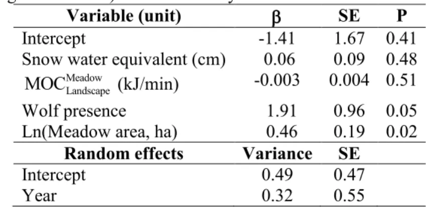
Our model explaining whether or not bison create feeding snow craters in meadows had “good” predictability, with an AUC = 0.84. The model indicated that the probability of bison foraging in a meadow (i.e., created at least one feeding crater) increased with meadow area (Table 1). Further, meadows in which bison foraged were more likely to be

visited by wolves. We did not detect any significant relationship with MOC or SWE (Table 1).

Table 1: Coefficients and standard errors for mixed-effects logistic regression model

predicting the probability that bison foraged in a given meadow in Prince Albert National Park (Saskatchewan, Canada) during the winters of 1997, 1998 and 2011. Independent variables included snow water equivalent, missed opportunity costs of foraging in that meadow and not elsewhere ( Meadow

Landscape

MOC ), wolf presence (absence = 0, presence = 1) and meadow area (log-transformed). N = 221 surveys in 26 meadows.

Variable (unit)  SE P

Intercept -1.41 1.67 0.41

Snow water equivalent (cm) 0.06 0.09 0.48 Meadow

Landscape

MOC (kJ/min) -0.003 0.004 0.51

Wolf presence 1.91 0.96 0.05

Ln(Meadow area, ha) 0.46 0.19 0.02

Random effects Variance SE

Intercept 0.49 0.47

Year 0.32 0.55

Foraging intensity

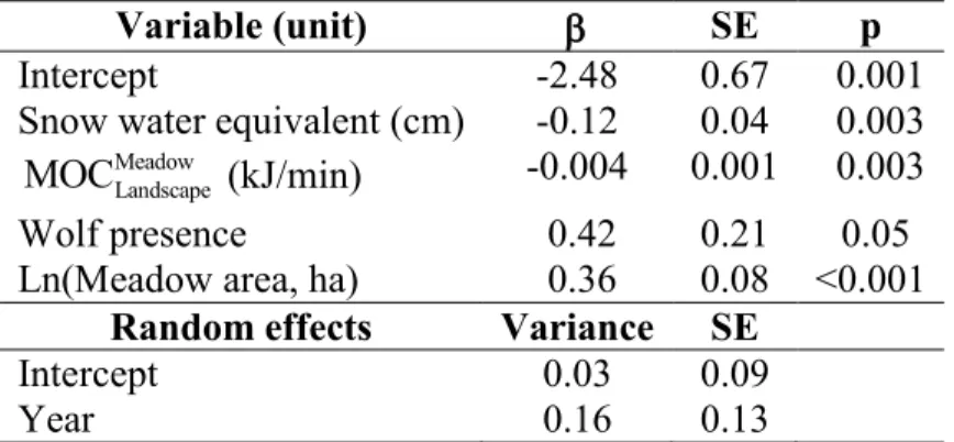
Once foraging in a meadow, bison created larger craters if the Meadow Landscape

MOC of

foraging in that meadow was relatively low (Table 2). Feeding intensity further increased in meadows with relatively low SWE. Bison also created larger crater areas in larger meadows (Table 2), but this increase was at a diminishing rate. First, the increase relationship was stronger (AIC = 90.8) with log-transformed meadow area (AIC = -128.9) than without any transformation (AIC = -38.1).Second, the proportion of meadows comprised of craters (Prop) decreased with meadow area: arcsine(Prop)0.5 = 0.25 - 0.02(SWE) - 0.0007(

Meadow Landscape

MOC ) + 0.04(Wolf Presence) - 0.08ln(Meadow Size) (n = 144 ratios and Pseudo R2 =0.46, all coefficients had P<0.05, except for wolf presence and intercept). These findings indicate that, although bison make larger craters in large than small meadows, there was a larger area without foraging activity in large meadows. Moreover, the proportion of ungrazed feeding stations with profitability higher than the landscape’s average was similar in small and large meadows: arcsine(Prop_quadrats)0.5 = 0.83 - 0.007ln(MS) (P = 0.88, n =

45). In other words, after leaving, bison left more vegetation of relative high profitability in large than in small meadows.

Finally, we found that bison foraged more intensively in meadows where we found wolf sign than where we did not (Table 2). This relationship indicates that both species made intensive use of the same meadows. Indeed, using radio-telemetry, we found that the relative probability of occurrence of radio-collared bison (p) increased with the utilization distribution of radio-collared wolves (UD): p/(1-p) = -0.45 + 2.57(UD) (P <0.0001; n = 18 716 bison locations for 23 female bison). This model was robust to cross-validation ( r_s = 0.82 ± 0.10).

Table 2: Coefficients and standard errors of a linear mixed effects model relating total

log-transformed crater area (ha) in individual meadows to snow water equivalent, missed opportunity costs of foraging in that meadow and not elsewhere ( Meadow

Landscape

MOC ), wolf presence (absence = 0, presence = 1) and meadow area (log-transformed). A total of 144 snow craters were recorded in 26 meadows in Prince Albert National Park (Saskatchewan, Canada) during the winters of 1997, 1998 and 2011. Pseudo R2 = 0.60.

Variable (unit)  SE p

Intercept -2.48 0.67 0.001

Snow water equivalent (cm) -0.12 0.04 0.003 Meadow

Landscape

MOC (kJ/min) -0.004 0.001 0.003

Wolf presence 0.42 0.21 0.05

Ln(Meadow area, ha) 0.36 0.08 <0.001

Random effects Variance SE

Intercept 0.03 0.09

Year 0.16 0.13

Plant biomass consumed in individual craters

The model of plant biomass consumed in individual craters with the most empirical support included missed opportunity costs at a global rather than a local scale (Table 3).

Table 3: Relative level of support by competing models explaining plant biomass

consumed in craters by plains bison in Prince Albert National Park (Saskatchewan, Canada) during the winters of 1997, 1998 and 2011. Differences in AIC (AIC) between the current model and the lowest scoring model are presented.

Hypothesis Model AIC AIC Rank

H1: ELandscape - EPatch _{SWE +} Patch Landscape

MOC + Wolf + ln(MS) 3132.8 0 1 H2: EMeadow - EPatch _{SWE +} Patch

Meadow

MOC + Wolf + ln(MS) 3148.7 15.9 2

Note: E = Plant profitability, SWE = Snow water equivalent, MOC = Missed opportunity costs, Wolf = Index of wolf presence, ln(MS) = Meadow size (log-transformed).

The top-ranking model (H1, Table 3) indicates that bison ate less vegetation in patches where global missed opportunity costs ( Patch

Landscape

MOC ) and SWE were high and where there was evidence of wolf presence (Table 4).

Table 4: Coefficients and standard errors for the top-ranking mixed effects linear model

relating average plant biomass consumed in a crater (g/m2) to snow water equivalent, global MOC ( Patch

Landscape

MOC ), wolf presence (absence = 0, presence = 1) and meadow area (log-transformed). A total of 262 quadrats of plant biomass were assessed in individual craters comprised in 26 meadows in Prince Albert National Park (Saskatchewan, Canada) during the winters of 1997, 1998 and 2011. Pseudo R2 = 0.65.

Variable (unit)  SE P

Intercept 75.68 26.84 0.02

Snow water equivalent (cm) -15.25 2.85 <.0001 Patch

Landscape

MOC (kJ/min) -0.54 0.05 <.0001

Wolf presence -44.19 18.09 0.02

Ln(Meadow area, ha) -10.11 6.06 0.10

Random effects Variance SE

Intercept 0

Year 315.37 631.49

DISCUSSION

By relating feeding efforts to energy (C), missed opportunity (MOC) and predation (P) costs of foraging, we showed that the strength of plant-bison interactions is largely driven by the search of bison for high net energy gains (C and MOC) and, to a lesser extent, by their management of predation risk. Our assessment of the foraging behaviour of free-ranging animals in a natural setting underscores the complex nature of the trophic interactions, and reveals spatial determinants of plant-herbivore interaction strengths.

Energy costs of foraging (C) and meadow attributes

Snow water equivalent (SWE) did not influence the probability that bison used a particular meadow. Once in a meadow, however, bison foraged over smaller areas if SWE was relatively high, and consumed less vegetation in craters where SWE was relatively high, a result consistent with previous reports (Fortin 2003, Fortin et al. 2003, Fortin and Fortin 2009). A high SWE imposes a high energy cost (Parker et al. 1984, Boertje 1985, Fancy and White 1985), and large herbivores tend to adjust foraging efforts to spatial patterns in snow conditions (Schaefer and Messier 1995, Fortin 2003, Fortin et al. 2005).

To reduce travel costs and increase the rate of energy intake, bison should benefit from foraging more intensively in areas where highly profitable food is concentrated. This objective can explain the influence of landscape physiognomy on plant-herbivore interactions. Bison were more likely to use large than small meadows, and they used larger meadows more intensively. Factors controlling meadow characteristics thus determine, to a certain extent, the strength of bison herbivory. The shape and size of meadows in Prince Albert National Park result from ecological succession that followed the retreat of Laurentide glacier, during late Pleistocene (Flint 1971, Strong and Hills 2005). Meadow dynamics are now linked to multiple processes. Beaver activity can create or maintain meadows (Pinay and Naiman 1991, Naiman et al. 1994, Westbrook et al. 2011), and fire helps maintain meadows by eliminating woody plants (Bailey and Wroe 1974, Anderson and Bailey 1980, Taylor et al. 2012). In absence of a natural fire and beaver activities, meadows gradually decrease in size due to tree and shrub encroachment (Bailey and Wroe 1974, Anderson and Bailey 1980), a process that induces a gradual loss of high-quality foraging patches for bison. Spatial variation in the strength of bison-plant interactions are thus linked to abiotic (e.g., fire and geological processes) and biotic factors (e.g. shrub encroachment, beaver activity), through their influence on meadow dynamics.

Missed opportunity costs (MOC)

MOC did not influence whether or not bison used a particular meadow. Once in a meadow, however, they fed more intensively (i.e., larger area covered by craters) if

Meadow Landscape