MARIE-CLAUDE LABBE
Jeu prédateur-proie entre le caribou forestier et le loup
gris : un effet saute-mouton spatialement structuré
Mémoire présenté
à la Faculté des études supérieures et postdoctorales de l'Université Laval dans le cadre du programme de maîtrise en biologie
pour l'obtention du grade de Maître es sciences (M.Sc)
DEPARTEMENT DE BIOLOGIE FACULTÉ DES SCIENCES ET DE GÉNIE
UNIVERSITÉ LAVAL QUÉBEC
2012 © Marie-Claude Labbé, 2012
RESUME
Cette étude a évalué le jeu spatial entre le caribou forestier et le loup gris en forêt boréale. Nous avons étudié les déplacements de 31 caribous et 16 loups de l'automne au printemps, lorsque le caribou s'alimente principalement de lichen. Nos analyses indiquent que, dans les zones utilisées fortement par le loup, ce prédateur sélectionnait généralement les secteurs riches en lichen, alors que le caribou orientait ses déplacements vers les coupes forestières. La théorie des jeux qualifie d'effet saute-mouton cette réaction simultanée des deux espèces. Cet effet disparaissait toutefois dans les zones moins utilisées par le loup, car le caribou sélectionnait alors les secteurs riches en lichen. Ainsi, le jeu entre le caribou et le loup se caractérisait par un effet saute-mouton spatialement structuré. L'évaluation de la disponibilité des ressources alimentaires pour les populations vulnérables du caribou devrait donc tenir compte de l'impact du loup sur l'accessibilité de la nourriture.
ABSTRACT
The aim of this study was to evaluate spatial game between the forest-dwelling caribou and gray wolves in the boreal forest. We studied the movements of 31 caribou and 16 wolves from autumn to spring, when caribou feed mainly on lichen. We found that, in areas heavily used by wolves, this predator selected mostly lichen-rich patches, while caribou oriented their movements towards forest cuts. Game theory describes this combined response of the two species as a leapfrog effect. This effect disappeared, however, in areas used less intensively by wolves, because caribou selected lichen-rich patches in those areas. Thus, the game between caribou and wolves was characterised by a spatially structured leapfrog effect. The assessment of food available to threatened populations of forest-dwelling caribou should consider how the spatial organisation of wolves limits resource accessibility.
AVANT-PROPOS
Ce mémoire de maîtrise vise à mieux comprendre l'influence du risque de prédation par le loup gris sur le caribou forestier, un écotype considéré comme vulnérable au Québec. Ce mémoire est divisé en trois parties distinctes : une introduction générale, un chapitre principal présenté sous forme d'article scientifique rédigé en anglais et une conclusion générale. La recherche du chapitre principal a été entreprise en collaboration avec plusieurs chercheurs :
- Daniel Fortin, directeur de maîtrise et professeur au département de biologie de l'Université Laval.
Mathieu Basille, post-doctorant au département de biologie de l'Université Laval.
Christian Dussault, chercheur biologiste au Ministère des Ressources naturelles et de la Faune et professeur associé de l'Université Laval.
Réhaume Courtois, chercheur biologiste au Ministère des Ressources naturelles et de la Faune.
James D. Forester, professeur au département de « Fisheries, Wildlife, and Conservation Biology » de l'Université du Minnesota.
Remerciements
Tout d'abord, je tiens à remercier mon directeur de recherche, Daniel Fortin, pour son aide précieuse, sa grande disponibilité et son soutien au cours de mon apprentissage. Durant ces dernières années, il fut toujours très ouvert à mes différents projets. Je suis très reconnaissante et je le remercie de m'avoir donné l'opportunité d'entreprendre ces études graduées au sein de son laboratoire.
J'aimerais également remercier Mathieu Basille, sans qui ce projet de maîtrise n'aurait pas été le même. Sa patience lors de mon apprentissage fut admirable et très appréciée. Mathieu m'a toujours poussé à aller plus loin et m'a aidé à affronter mes craintes.
Je suis également bien reconnaissante à James D. Forester de m'avoir accueilli dans son laboratoire lors d'un stage à l'Université du Minnesota. Toujours très ouvert à mes discussions et interrogations, il aura été un hôte exemplaire. Ce fut une expérience mémorable, enrichissante et très appréciée.
Je tiens aussi à remercier Christian Dussault, Réhaume Courtois et Jean-Pierre Ouellet pour m'avoir donné des commentaires constructifs sur mes différents travaux tout au long de ma maîtrise. Plus particulièrement, un grand merci à Christian pour ses suggestions sur mon proposé de projet de recherche et pour m'avoir accueilli au bureau du Ministère des Ressources naturelle et de la Faune durant quelques jours afin de me permettre de mieux comprendre le fonctionnement et le rôle du ministère.
Je tiens à remercier Jean-Pierre Tremblay pour ses suggestions sur mon proposé de projet de recherche. Je souhaite également remercier Steeve Côté et Martin-Hugues St-Laurent qui ont accepté d'évaluer ce mémoire.
Je remercie les gens qui ont fait partie du laboratoire au cours des deux dernières années : Mathieu Basille, Guillaume Bastille-Rousseau, Orphé Bichet, Sabrina Courant, Nicolas Courbin, Karine Dancose, Angélique Dupuch, Léa Harvey, Hélène Le Borgne, Chrystel Losier, Aurore Malapert, Jerod Merkle, Guillaume Moreau, Carolyn Nersesian, Marie Sigaud, Kyle Swiston, Olivia Tardy, Qing Zhao ainsi que leurs conjoints/conjointes, ami/amie, famille, etc. Les discussions et commentaires que vous m'avez offerts sur mes présentations, mon proposé de maîtrise et mon mémoire m'ont grandement appris. De plus, les dîners, soirées et autres activités passés avec vous ont toujours été agréables et enrichissants. L'ambiance, le dynamisme et la complicité que nous avons développés me seront toujours un souvenir du bon temps passé en bonne compagnie!
Finalement, du plus profond de mon âme, je tiens à remercier ma famille et mes amis qui, tout au long de ces années, m'ont supporté et encouragé à toujours aller plus loin. À mon père, pour son éternel soutien et pour croire qu'on peut affronter l'insurmontable un jour à la fois. Pour aussi m'avoir partagé son amour de la nature. À ma mère pour son écoute inconditionnelle et sa tendresse. À mon frère pour m'avoir ouvert la porte sur les études supérieures. Vous êtes tous un modèle à mes yeux. Et finalement à mon copain, je le remercie pour son soutien et sa patience lors de mes nuits de travail et mes escapades lors de conférences.
Merci à tous, et maintenant : bonne lecture!
« And the day came when the risk to remain tight in a bud
was more painful than the risk it took to blossom »
Anaïs Nin (1903 -1977)
TABLE DES MATIERES
RESUME III ABSTRACT IV AVANT-PROPOS V
REMERCIEMENTS VI TABLE DES MATIÈRES IX LISTE DES TABLEAUX X LISTE DES FIGURES XI INTRODUCTION 1
I. CONTEXTE THÉORIQUE 1
Sélection d'habitat et déplacements 1 Interactions prédateur-proie 2
II. DÉPLACEMENTS DU CARIBOU FORESTIER 5
III. OBJECTIF DE L'ÉTUDE 7
Hypothèse et prédictions 7
IV. APPROCHES EMPIRIQUES 8
Jeu spatial entre prédateur et proie 8
Prédateur 9 Proie 9
CHAPITRE PRINCIPAL 11 SPATIALLY STRUCTURED LEAPFROG EFFECTS IN THE SPATIAL GAME BETWEEN
THREATENED WOODLAND CARIBOU AND GRAY WOLVES 11
I. ABSTRACT 12 II. INTRODUCTION 13 III. METHODS 16
Study Area 16 Telemetry data 17 Co-occurrence between caribou and wolves 17
Habitat description 19 Habitat selection of wolf. 19 Movements of caribou 20
IV. RESULTS 22
Co-occurrence between caribou and wolves 22
Habitat selection of wolves 23 Movements of caribou 25
V. DISCUSSION 29 VI. ACKNOWLEDGEMENTS 32
VII. REFERENCES 32 CONCLUSION GÉNÉRALE 39
I. JEU SPATIAL - EFFET SAUTE-MOUTON STRUCTURÉ 39
II. IMPLICATIONS POUR LA CONSERVATION 42
III. ORIGINALITÉ DU PROJET 45
IV. PERSPECTIVES 46 BIBLIOGRAPHIE DE L'INTRODUCTION ET DE LA CONCLUSION 48
LISTE DES TABLEAUX
Table 1 Cover percentage in the study area in managed boreal forests 16
Table 2 Coefficients (|3) and standard errors (SE) of mixed-effects logistic regression models of resource selection by gray wolves in managed boreal forests for three biological seasons of the year. The model accounts for multiple landscape features, as well as for changes in the selection of open conifer stands with lichen as a function of the wolf utilization distributions (UD). The /(-fold average values (7"s values ± SE) for
the cross validation are also reported 24
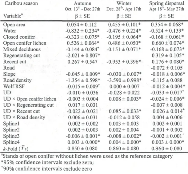
Table 3 Coefficients (P) and robust standard errors (SE) for step selection functions of forest-dwelling caribou in managed boreal forests for three biological seasons. Wolf utilization distributions (UD) were obtained using kernel methods whereas the wolf resource selection function (Wolf RSF, Table 2) was obtained using a generalized linear mixed model. A 3-knot linear spline function of distance moved has been added to the model. The /(-fold values [l"s values ± SE) for the cross validation are also
LISTE DES FIGURES
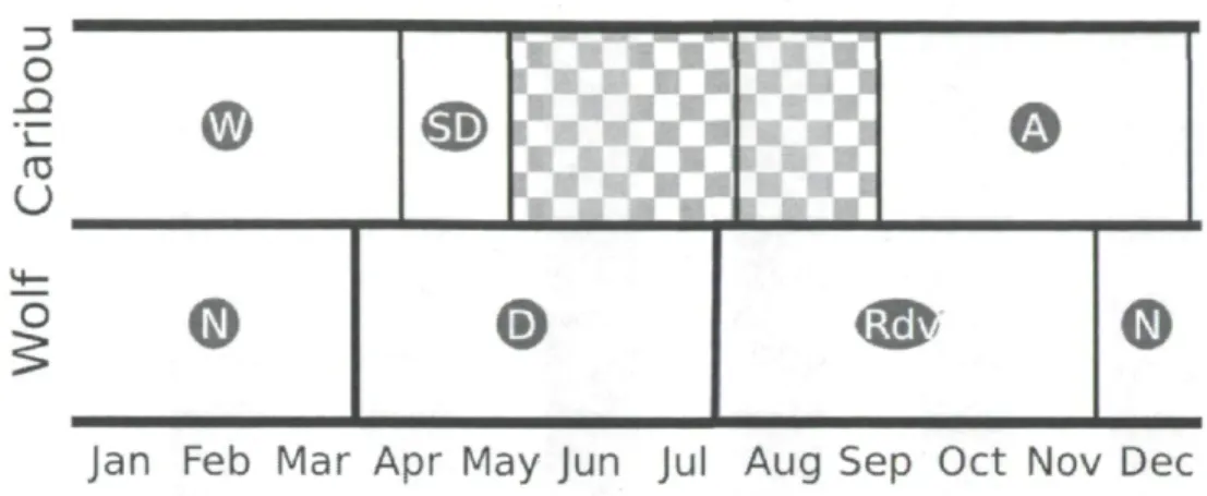
Figure 1: Representation of the biological seasons for caribou and wolves throughout the year in boreal forest of Quebec, Canada. The region shaded in grey represents two seasons that were not considered in our study because lichen is not the dominant food source for caribou during that time. Legends: W = winter, SD = spring dispersal,
A = autumn, N = nomadic, D = denning, Rdv = rendezvous 19
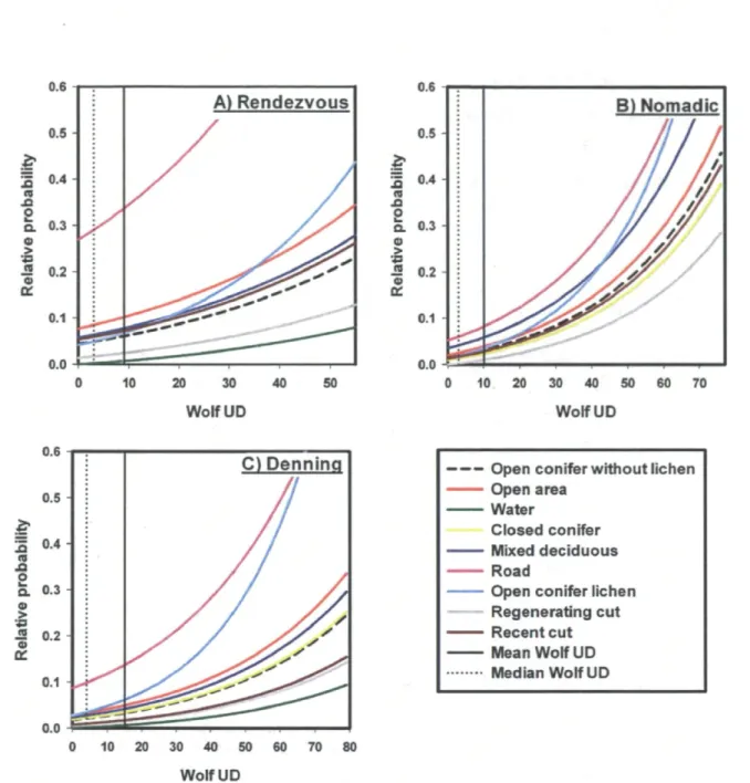
Figure 2: Relative probability of occurrence for various land cover types as a function of the wolf utilization distribution (UD) in the boreal forest of Quebec (Canada),
during: A) the rendezvous, B) nomadic, and C) denning seasons 25
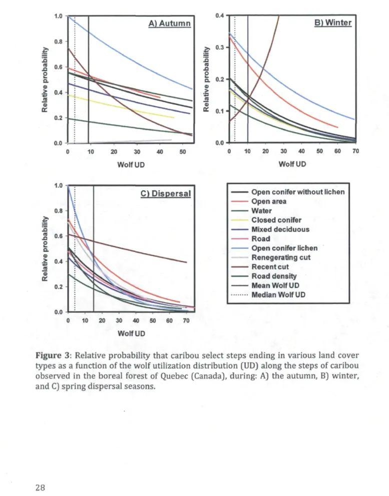
Figure 3: Relative probability that caribou select steps ending in various land cover types as a function of the wolf utilization distribution (UD) along the steps of caribou observed in the boreal forest of Quebec (Canada), during: A) the autumn, B) winter,
and C) spring dispersal seasons 28
INTRODUCTION
I. Contexte théorique
Sélection d'habitat et déplacements
La compréhension de la répartition spatiale des espèces est primordiale à l'élaboration de mesures de gestion et de conservation efficaces (Mitchell et Lima 2002). La répartition des animaux est largement influencée par leur sélection d'habitat (Mayor et al. 2009), qu'on définit comme une utilisation disproportionnée de composantes de l'habitat par rapport à leur disponibilité dans le paysage (Johnson 1980). La plupart des animaux doivent combler simultanément plusieurs besoins tels que l'acquisition de nourriture, l'évitement des prédateurs et la recherche de partenaires sexuels (Bennett 1998). Les compromis que cette multitude de besoins implique, et la sélection d'habitat qui s'ensuit, entraînent généralement une répartition hétérogène de ces animaux, à la fois dans le temps et dans l'espace.
Les déplacements sont à la base du processus de sélection de l'habitat. Ces déplacements sont influencés non seulement par les types de milieu que les animaux recherchent, mais également par les milieux qu'ils doivent traverser pour se rendre aux parcelles visées (Kotliar et Wiens 1990, Wiens et al. 1997). Les déplacements sont donc influencés par la structure du paysage, de même que par la dynamique de changement de cette structure (p. ex. : le degré de fragmentation, Johnson et al. 1992). L'étude des déplacements des animaux peut donc nous informer sur l'influence qu'exercent les composantes environnementales sur les compromis exprimés par les animaux et, éventuellement, sur la dynamique de la répartition spatiale des individus (Wiens et al. 1997). Toutefois, la plupart des études portant sur la sélection d'habitat n'évaluent pas directement comment les animaux ajustent leurs déplacements aux patrons d'hétérogénéité de l'habitat.
De façon générale, les proies peuvent se déplacer afin de se disperser dans leur habitat (Zollner et Lima 1999), de patrouiller leur territoire (Boinski et Garber 2000) ou de trouver un partenaire sexuel (Daly et al. 1990). Ces déplacements ne se font toutefois pas sans risque. Dans un environnement où prédateurs et proies se côtoient, les déplacements des proies peuvent attirer l'attention des prédateurs (Skelly 1994). Les proies doivent donc adopter des comportements reflétant un compromis entre l'accès à la ressource et le risque de prédation.
Interactions prédateur-proie
L'utilisation d'un même type de milieu par les prédateurs et par les proies peut mener à leur interaction, et définir la nature de ces interactions est essentiel à notre compréhension du fonctionnement des réseaux trophiques. Plusieurs études se sont donc penchées sur les effets létaux que les prédateurs ont sur leurs proies (Hazzard et al. 1991, Oedekoven et Joern 1998, Hallfredsson et Pedersen 2009). Pourtant, bien que la mort soit un aspect fondamental des interactions entre prédateurs et proies, une compréhension complète de ces interactions nécessite également une connaissance des effets non létaux des prédateurs (Lima 1998). Effectivement, les effets non létaux peuvent parfois être plus importants que les effets létaux sur le réseau trophique (Trussell et al. 2006, Creel et Christianson 2008) en causant, par exemple, des cascades trophiques d'origine comportementale. Au cours de la dernière décennie, de nombreux chercheurs ont étudié les effets indirects de la prédation (Schmitz 1998, Valeix et al. 2009, Fanson 2010). Parmi les réactions comportementales possibles d'une proie face au risque de prédation, nous retrouvons un changement de sa répartition spatiale (Ripple et Beschta 2004), la sélection d'un type de milieu spécifique (Creel et al. 2005), les changements temporels et spatiaux dans les budgets d'activité (Fenn et Macdonald 1995), l'ajustement des règles de déplacement (Fortin et al. 2005), la réduction des taux de déplacements (Sih et McCarthy 2002), l'adoption d'un comportement plus grégaire (Lima 1995), l'augmentation du temps alloué à la vigilance (Périquet et al. 2010) et la diminution
du temps consacré à la recherche de nourriture (Abramsky et al. 2002). De façon générale, la proie modifie son comportement en fonction de la perception qu'elle a du risque de prédation de manière à diminuer ses probabilités de rencontre avec le prédateur, d'être détectée par le prédateur ou même de se faire capturer par ce prédateur (Lima et Dill 1990).
Selon Linnell et Strand (2000), la répartition spatiale de la proie reflète principalement le compromis entre l'apport énergétique, la compétition intraspécifique et le risque de prédation. Afin de réduire le risque chronique de prédation, la proie doit éviter au maximum les opportunités de rencontre avec son prédateur; elle doit pour cela éviter les zones les plus utilisées par le carnivore (Lima et Dill 1990, Jeschke et al. 2008). Une rencontre peut survenir lorsque les divers compromis que la proie doit effectuer la sollicite néanmoins à s'aventurer dans ces zones. La proie peut alors tenter de réduire la probabilité d'être effectivement détectée par son prédateur lorsqu'elle circule dans ces zones risquées (Jeschke et al. 2008). Des études ont montré que certains herbivores utilisent différents types de milieu en fonction du risque de prédation à court terme associé à chaque type de milieu (Lima 2002, Wirsing et al. 2007, Valeix et al. 2009). Par exemple, ils peuvent sélectionner des milieux ouverts où la détection d'un prédateur qui s'approcherait est plus facile et, de ce fait, échapper plus efficacement à une attaque (Valeix et al. 2009).
Les interactions entre les prédateurs et les proies peuvent être dynamiques dans l'espace et le temps (Linnell et Strand 2000, Lima 2002, Dupuch et al. 2009, Valeix et al. 2009). Par exemple, une proie peut jouer au jeu de passe-passe («shell game », Mitchell et Lima 2002) en étant constamment en déplacement pour empêcher les prédateurs de prévoir sa position dans le paysage à un moment donné (Mitchell et Lima 2002, Laundré 2010). L'efficacité de la proie à éviter un prédateur dépend aussi de la réaction de ce prédateur. Le jeu spatial entre prédateur et proie peut donc produire différents résultats. Par exemple, il y a généralement une
cooccurrence spatiale entre le guillemot (Uria spp.) et sa proie, le capelan (Mallotus villosus), dans la mer de Barents (Fauchald et al. 2000). Au contraire, il y a ségrégation spatiale entre le cougar (Puma concolor) et sa proie, le cerf mulet (Odocoileus hemionus) dans l'Utah et l'Idaho (Laundré 2010). Il existe donc une certaine variabilité dans le dénouement du jeu spatial entre les prédateurs et les proies.
Cette variabilité souligne des différences de gagnant dans le jeu spatial qui prend place entre prédateurs et proies (Sih 2005, Laundré 2010). Selon Sih (2005), le « gagnant » du jeu spatial entre un prédateur et sa proie peut être identifié par des modèles de cooccurrence entre les espèces. La proie est considérée comme gagnante du jeu lorsqu'il y a une association spatiale négative entre le prédateur et la proie, alors que le prédateur est le gagnant du jeu lorsqu'il y a une association spatiale positive entre les deux (Sih 2005). Les prédateurs peuvent profiter du fait que les parcelles de haute qualité peuvent parfois être clairement définies pour une proie. Dans ce cas, les parcelles peuvent être considérées comme des « points d'ancrage » (sensu Sih 2005) pour les proies. Un point d'ancrage représente une caractéristique du paysage, comme une parcelle autour de laquelle peuvent s'organiser les déplacements des animaux. Un bon exemple de points d'ancrage est donné par les points d'eau dans les environnements arides (Valeix et al. 2009). Ces points d'ancrage de la proie peuvent alors être utilisés par les prédateurs pour y concentrer leur recherche puisque les probabilités de rencontrer la proie sont élevées. Cet attrait du prédateur pour la ressource de la proie peut sembler contre-intuitif, particulièrement lorsque le prédateur ne consomme pas cette ressource (p. ex. : ressource végétale). D'autant plus que la proie peut être relativement peu abondante dans ces sites riches en nourriture. En effet, la réaction des proies au risque de prédation donne parfois lieu à l'effet saute-mouton (Sih 1998), par lequel les prédateurs sélectionnent les secteurs où abondent les ressources de la proie, tandis que les proies évitent ces sites riches en ressources afin de réduire leur risque de prédation (Sih 1998, Hammond et al. 2007, Laundré 2010).
Les prédateurs font également face à certaines contraintes spatiales. Par exemple, l'utilisation des tanières et l'évitement des compétiteurs ou des êtres humains peuvent façonner la dynamique de la répartition spatiale des prédateurs (Lima 2002, Hebblewhite et Merrill 2009, Muhly et al. 2011). Les zones tampons entre les territoires de prédateur (Mech 1977, Taylor et Pekins 1991, Lewis et Murray 1993, Mech et Boitani 2003) ou les zones d'activités humaines (White et al. 1998) peuvent d'ailleurs agir comme un refuge pour les ongulés. Une ségrégation spatiale pourrait alors se produire entre le prédateur et sa proie dans ces régions spécifiques, et ainsi la proie gagnerait le jeu spatial, au prix d'un évitement des zones les plus riches en nourriture.
II. Déplacements du caribou forestier
Les populations du caribou forestier (Rangifer tarandus caribou) sont considérées comme menacées au Canada (COSEPAC 2002) depuis 2002 (loi sur les espèces en péril, LEP) et comme vulnérables au Québec depuis 2005 (Loi sur les espèces menacées et vulnérables du Québec, Décret 75-2005). En raison de l'état précaire des populations, plusieurs études ont été réalisées pour mieux comprendre la répartition spatiale et la sélection d'habitat du caribou forestier (Seip 1992, Rettie et Messier 2000, Ferguson et Elkie 2004, James et al. 2004, Courtois et al. 2007, Wittmer et al. 2007, Fortin et al. 2008, Hins et al. 2009, Courbin et al. 2009, Festa-Bianchet et al. 2011). Le déclin des populations s'expliquerait en grande partie par l'aménagement forestier. Cet aménagement entraîne d'une part une altération directe de l'habitat du caribou et, d'autre part, une augmentation de l'abondance du loup gris (Canis lupus), un prédateur du caribou qui limite souvent les populations de ses proies (Seip 1992, Wittmer et al. 2005). Cette augmentation du prédateur est due au fait que la régénération des coupes forestières apporte souvent une forte abondance de ressources alimentaires pour l'orignal (Alces alces). Il peut donc s'en suivre un plus fort recrutement d'orignaux, susceptible d'entraîner une augmentation des populations de loups (Messier 1994, Tremblay et al. 2001) et, par conséquence, un
risque de prédation accru pour le caribou (Wittmer et al. 2007). Ce processus est connu sous le nom de compétition apparente. Selon ce type de compétition, l'effet d'une espèce sur une autre ne se fait pas par des interactions directes, mais de façon indirecte, par l'intermédiaire d'un prédateur commun (Holt 1977, DeCesare et al. 2010).
Pour diminuer les effets du risque de prédation, les ongulés peuvent éviter les zones d'activité intensive de leurs prédateurs (Hernandez et Laundré 2005). Les caribous pourraient donc maximiser leur aptitude phénotypique en évitant de se déplacer vers les zones qui sont plus utilisées par le loup et l'ours noir. En effet, le loup consomme des caribous de tout âge durant toute l'année (Cumming 1992, Courtois et al. 2007), tandis que l'ours noir (Ursus americanus) se nourrit de nouveau-nés durant la période de mise bas (Pinard et al. 2012). Les caribous doivent toutefois aussi combler leurs besoins alimentaires. Pendant l'automne, l'hiver et à la dispersion printanière, ils consomment principalement du lichen (Crête et al. 1990). Cette nourriture est particulièrement abondante dans les landes à lichens et certains peuplements de conifères (Courtois 2003). Pendant le reste de l'année, le caribou consomme des feuilles d'arbustes qui sont réparties plus largement dans l'environnement (Crête et al. 1990). Les parcelles riches en nourriture pour le caribou peuvent donc être clairement définies de l'automne à la dispersion printanière et pourraient fournir aux prédateurs des zones où concentrer leur effort de chasse.
Le loup est reconnu comme étant un prédateur au sommet de la chaîne alimentaire en forêt boréale (Houle et al. 2010). Au Québec, l'orignal constitue sa proie principale (Tremblay et al. 2001), alors que le caribou, le castor (Castor canadensis) et le lièvre (Lepus americanus) sont habituellement des proies alternatives (Larivière et al. 2000). Malgré cela, l'impact du loup sur les populations de caribou peut être très important puisque la prédation par le loup constitue la première cause de mortalité chez les caribous adultes (Seip 1992, Lambert et al.
2006). La sélection d'habitat de ce prédateur varie selon les saisons et impose une contrainte au caribou, particulièrement à l'hiver, alors que la probabilité de cooccurrence entre les deux espèces est la plus élevée (Courbin et al. 2009) et au cours du printemps lorsque les interactions entre le loup et l'orignal sont au plus faible (Basille et al. 2012). Durant cette période, il est donc probable que les déplacements du caribou soient influencés par la probabilité d'occurrence du loup. Peu d'études ont toutefois porté sur les déplacements du caribou forestier en fonction du risque de prédation.
III. Objectif de l'étude
Le but principal de notre projet était d'identifier l'influence du risque de prédation sur les déplacements du caribou forestier. Plus précisément, nous avons évalué le jeu spatial entre le caribou forestier et le loup gris dans la forêt boréale de l'est du Canada, notamment en identifiant le gagnant du jeu spatial d'une façon générale, de même que les changements dans le temps et dans l'espace qui caractérisent ce jeu prédateur-proie.
Hypothèse et prédictions
Nous émettons l'hypothèse que le jeu spatial qui prend place entre le loup et le caribou se caractérise par un effet saute-mouton spatialement structuré. Si tel était le cas, nous pourrions nous attendre à ce que les déplacements du caribou soient préférentiellement dirigés vers les forêts de conifères ouvertes à lichen lorsque le caribou se situe dans une région faiblement utilisée par le loup. Au contraire, le caribou devrait alors éviter les forêts de conifères ouvertes à lichen et trouver refuge dans les types de milieu qui sont peu ou pas utilisés par le loup lorsqu'il est dans une région fortement utilisée par le loup. La sélection des forêts de conifères ouvertes à lichen par le loup entraînerait alors un effet saute-mouton étant spatialement structuré. Bien que l'effet saute-mouton a été rapporté dans quelques études
(Sih 1998, Hammond et al. 2007, Hammond et al. 2012), le concept de structure spatiale dans cette résultante du jeu prédateur-proie n'avait pas encore été abordé.
IV. Approches empiriques
Pour atteindre notre objectif, nous avons suivi par télémétrie 31 femelles caribous et 16 loups associés à 8 meutes. Les analyses subséquentes ont été effectuées en considérant seulement les observations localisées dans les zones utilisées à la fois par le caribou et par le loup. Ce sous-échantillonnage a été fait puisque la population de loup n'étant pas intégralement suivie, nous ne pouvons pas garantir l'absence de loup dans les zones où aucune localisation n'a été relevée. Toutefois, puisque le loup est une espèce territoriale, notre suivi télémétrique nous permet d'établir les variations dans l'utilisation de l'espace pour chacune des meutes en suivant un nombre relativement restreint de leurs membres.
Jeu spatial entre prédateur et proie
Nous avons évalué le gagnant du jeu spatial entre le caribou et le loup, en évaluant si le caribou évite globalement les zones que le loup utilise de façon plus intensive. Pour estimer l'intensité d'utilisation du paysage par le loup au cours des saisons, nous avons utilisé les localisations GPS pour construire des fonctions de noyau (« kernel », Worton 1989) pour chacune des meutes et chacune des saisons à l'étude. Cet indice a ensuite été standardisé entre 0 et 100 pour cartographier l'utilisation relative du paysage par les prédateurs. Par la suite, nous avons testé si la probabilité d'occurrence du caribou variait en fonction de l'intensité d'utilisation du paysage par le loup. Si le caribou sort vainqueur du jeu, la probabilité d'occurrence du caribou devrait diminuer en fonction de l'intensité d'utilisation du paysage par le loup. L'inverse se produirait si le loup sortait vainqueur du jeu spatial.
Prédateur
Afin de déterminer si le prédateur sélectionne les parcelles riches en nourriture pour le caribou, un préalable essentiel à l'émergence d'un effet saute-mouton, nous avons étudié la sélection d'habitat du prédateur à l'aide des fonctions de sélection des ressources (« ressource selection functions », RSF, Manly et al. 2002). Trois saisons biologiques ont été considérées pour le loup: la période du rendez-vous (29 juillet au 16 novembre), la période nomade (27 novembre au 5 avril) et la période d'utilisation de la tanière (6 avril au 18 juillet). Les RSF permettent d'estimer la probabilité d'occurrence relative des individus dans un paysage hétérogène en fonction des caractéristiques spatiales de l'habitat (Manly et al. 2002). En pratique, nous avons comparé les caractéristiques des milieux fréquentés à celles des milieux disponibles. Cette disponibilité est généralement déterminée à l'aide de points lancés aléatoirement à l'intérieur des domaines vitaux (Boyce 2006), avec un ratio de 1:1 par rapport au nombre de localisations observées. Les localisations aléatoires informent sur la fréquentation de l'habitat attendue sous l'effet du hasard. La comparaison entre les attributs des localisations observées et aléatoires permet donc de déterminer les types de milieu sélectionnés et évités par le prédateur, selon ce qu'on peut s'attendre de façon aléatoire.
Proie
L'étude des déplacements de la proie durant l'automne (13 octobre au 27 décembre), l'hiver (28 décembre au 17 avril) et la dispersion printanière (18 avril au 27 mai) s'est effectuée grâce à des fonctions de sélection de pas (« step selection functions », SSF, Fortin et al. 2005). Les SSF permettent d'identifier les caractéristiques biotiques et abiotiques du paysage qui influencent les déplacements d'un animal. Les localisations permettent de spécifier les pas, qui sont alors définis comme les segments reliant les localisations successives prises selon un intervalle de temps fixe (Turchin 1998). Les SSF émergent de la comparaison entre les caractéristiques que l'on retrouve le long de pas faits par l'animal et les 9
caractéristiques de pas qui auraient pu être faits. Cette analyse nous a permis notamment de tester si l'influence des milieux riches en nourriture sur les déplacements du caribou variait selon l'intensité d'utilisation du paysage par le loup.
CHAPITRE PRINCIPAL
Spatially structured leapfrog effects in the spatial
game between threatened woodland caribou and
gray wolves
MARIE-CLAUDE LABBÉ1, DANIEL FORTIN1, MATHIEU BASILLE1, CHRISTIAN DUSSAULT2, RÉHAUME COURTOIS2 & JAMES D. FORESTER3
Chaire de Recherche Industrielle CRSNG-Université Laval en Sylviculture et Faune; Département de biologie; Université Laval; Québec, QC, G1V 0A6, Canada. MCL: marieclaude.m.labbe@gmail.com; DF: daniel.fortin@bio.ulaval.ca; MB: basille@ase-research.org
2Ministère des Ressources naturelles et de la Faune; Direction générale de l'expertise sur la faune et ses habitats; 880 chemin Sainte-Foy, 2e étage; Québec, QC, GIS 4X4,
Canada. CD: christian.dussault@mrnf.gouv.qc.ca; RC: rehaume.courtois@mrnf.gouv.qc.ca
d e p a r t m e n t of Fisheries, Wildlife, and Conservation Biology; University of Minnesota; 1980 Folwell Ave. St. Paul, MN 55108 USA. JDF: jdforest@umn.edu
I. Abstract
The spatial game between predators and prey can have a profound impact on food web properties. One of the outcomes of this spatial game is a leapfrog effect whereby predators match the distribution of their prey's resources instead of prey abundance itself, while prey undermatch their own resources to reduce risk. A number of studies have reported leapfrog effects, but few have shown or even tested for spatial structure in the strength of those effects. We investigated the spatial aspect of the behavioral response race between forest-dwelling woodland caribou (Rangifer tarandus caribou) and gray wolves (Canis lupus) from autumn to spring, when lichen is caribou's main food source. The movements of 31 radio-collared caribou and 16 radio-collared wolves from 8 packs were followed in boreal forest also occupied by moose (Alces alces). We found that caribou won the spatial game during autumn and winter by maintaining significant segregation from wolves. Caribou selected conifer stands rich in lichen in low wolf-use areas; however, in areas of high wolf use, caribou generally became more likely to move into recently cut forests than lichen-rich areas. Wolves selected open conifer stands with lichen, especially in areas that they used intensively. The caribou-wolf system was therefore characterized by spatially structured leapfrog effects, with those effects being strong in high wolf-use areas and vanishing in low wolf-use areas. In addition to providing one of the first empirical demonstrations of strong spatial heterogeneity in the leapfrog effect, our study indicates that food web complexity (i.e., presence of alternative prey) could give some advantage to the prey in the spatial game because predators then have multiple spatial targets. Predicting how these interactions play out can provide critical information to adequately assess the challenges that involve the preservation of threatened prey populations (such as forest-dwelling woodland caribou) through habitat management, especially when they are faced with strong top-down forces.
II. Introduction
The strong impact that nonlethal effects of prédation can have on food web properties is broadly recognized (Lima 1998, Schmitz 1998, Laundré et al. 2001, Laundré 2010). Prey may react to prédation risk in multiple ways, such as by increasing vigilance (Périquet et al. 2010), by reducing foraging time and food intake rate (Abramsky et al. 2002), and by adjusting their spatial distribution (Ripple and Beschta 2004) and habitat selection (Creel et al. 2005, Fortin et al. 2005). A striking example is the reintroduction of gray wolves (Canis lupus) to Yellowstone National Park, which has resulted in changes in the number (White et al. 2012) and spatial dynamics (Fortin et al. 2005) of the local elk [Cervus canadensis) population, with subsequent effects on the recruitment of woody browse species in some sections of the park (Ripple and Beschta 2004, Beschta and Ripple 2010, but see also Kauffman et al.2010).
Predators look for prey while prey attempt to avoid those encounters with their predators; these simple motivations may result in sophisticated games (Linnell and Strand 2000, Lima 2002, Dupuch et al. 2009, Valeix et al. 2009, Kotler et al. 2010). Prey may play a shell game by being constantly on the move to prevent predators from predicting their location (Mitchell and Lima 2002, Laundré 2010). Prey can also focus their activities in areas where an encounter with predators is less likely to occur (Lima 2002). The ability of prey to avoid those encounters depends, however, on the concurrent response of their predators. For example, murres (Uria spp.) tend to co-occur with capelin (Mallotus villosus) in the Barents Seas (Fauchald et al. 2000), whereas spatial segregation has been reported between mountain lions (Puma concolor) and mule deer (Odocoileus hemionus) in Utah and Idaho (Laundré 2010). These differences may reflect whether predators or prey are ahead in their spatial game (Sih 2005, Laundré 2010).
In the terminology of contests, this spatial game is a behavioral response race in which the "winner" can be identified by assessing patterns of co-occurrence between predator and prey. If prey win the game, the outcome is a negative spatial association between the two opponents, whereas if predators win, the association is positive (Sih 2005). Predators may take advantage of the fact that high-quality patches can be clearly defined for some prey, e.g. in terms of food resources. In this case, the good patches become "spatial anchors" for prey, which provide predators with specific locations where they can concentrate their search. This opportunity may give rise to the leapfrog effect (Sih 1998), whereby prey undermatch their own resources to reduce prédation risk while predators match the distribution of the prey's resource but not of the abundance of prey (Sih 1998, Hammond et al. 2007, Laundré 2010). On the other hand, predators also have their own set of spatial constraints. For example, the use of dens or the avoidance of competitors or humans may shape the spatial dynamics of predator distributions (Lima 2002, Hebblewhite and Merrill 2009, Muhly et al. 2011). Further, buffer zones between predator territories (Mech 1977, Taylor and Pekins 1991, Lewis and Murray 1993, Mech and Boitani 2003) or human activity centers (White et al. 1998) might act as a refuge for ungulates (Berger 2007). Spatial segregation would then occur in those specific areas, but not necessarily elsewhere.
Differences in spatial constraints and anchor points between predators and prey can therefore result in spatially structured leapfrog effects: species co-occurrence in patches rich in the prey's food is weak in parts of the landscape but strong in others. Such adaptive response might emerge when prey achieve fitness gains by undermatching resource distribution only in some areas of the landscape. Depending on multi-scale patterns of predator distribution, variations in the response of prey to the local predator distribution could occur within the home-range of an individual, among the home-ranges of population members, or simultaneously at both levels. Because movement is one of the most fundamental mechanisms underlying animal distributions (Turchin 1998), plasticity in the response of prey to predator 14
density should translate into particular risk-dependent movement rules. Specifically, a spatially structured leapfrog effect would occur when prey avoid moving towards food-rich patches in areas heavily used by predators (i.e., high values of the predator utilization distribution, UD), but do not undermatch their resources in low-risk areas (low UD). The concurrent selection of predators for the food-rich patches of their prey would then result in spatially structured leapfrog effects.
Here we assessed the spatial structure in the behavioral response race between forest-dwelling woodland caribou (Rangifer tarandus caribou) and gray wolves in eastern Canada. The forest-dwelling caribou is a threatened ecotype (COSEWIC 2002) with its populations generally being limited by prédation (Seip 1992, Wittmer et al. 2005) instead of food (Courtois et al. 2007). Therefore, caribou might experience strong fitness costs by moving towards areas of high risk of predator encounter. From autumn to spring, caribou mainly consume lichen (Crête et al. 1990, Johnson et al. 2001), which are especially abundant in some open conifer stands (hereafter referred to as open conifer stands with lichen). During the rest of the year, caribou mainly consume leaves of shrubs (Crête et al. 1990). Because food-rich patches can be clearly defined for caribou during autumn, winter, and the spring dispersal (but not as well for other times of the year), we restricted our analysis to these three biological seasons. The gray wolf is the only relevant predator of caribou during these seasons. If spatially structured leapfrog effects characterize the wolf-caribou spatial game, we would expect wolf-caribou to bias their movements towards open conifer stands with lichen when they are in areas of low wolf use, but not in areas of high wolf use. In areas of high predator UD, prey should find refuge in forest stands avoided by wolves. Therefore, simultaneous selection of open conifer stands with lichen by wolves would result in a spatially structured leapfrog effect.
III. Methods Study Area
The study area covered approximately 23,600 km2 over two main sectors located in the boreal forest in eastern Québec, Canada (46-51°N, 68-71°W). The forest landscape consisted of a matrix of mature conifer stands dominated by balsam fir (Abies balsamea) and black spruce (Picea mariana). The remaining primarily consists of coniferous stands dominated by jack pine (Pinus banksiana), deciduous or mixed stands dominated by white birch (Betula papyrifera) and aspen (Populus tremuloides), regenerating sites, water bodies, and open areas (Table 1). Forestry practices created a gradient in logging intensity from South-West to North-East, with 25% to 4% of the area having been harvested in the past 30 years (Basille et al. 2010). The elevation ranges from 250 to 1100 m above sea-level and the average temperatures range from -23 °C in January to 14 °C in July. In the south-western portion of the study area, the average annual rainfall is 150 cm with more than 2 m of snowfall during the cold seasons (Houle et al. 2010), whereas the north-eastern annual rainfall averages 71 cm (Crête and Courtois 1997) with a mean snowfall reaching a maximum of 1 m in March (Courbin etal. 2009).
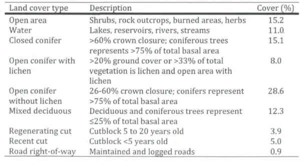
Table 1 Cover percentage in the study area in managed boreal forests.
Land cover type Description Cover (%) Open area Shrubs, rock outcrops, burned areas, herbs 15.2
Water Lakes, reservoirs, rivers, streams 11.0. Closed conifer >60% crown closure; coniferous trees 15.1
represents >75% of total basal area
Open conifer with >20% ground cover or >33% of total 8.0 lichen vegetation is lichen and open area with
lichen
Open conifer 26-60% crown closure; conifers represent 28.6 without lichen >75% of total basal area
Mixed deciduous Deciduous and coniferous trees represent 12.3 <25% of total basal area
Regenerating cut Cutblock5 to 20 years old 3.9 Recent cut Cutblock <5 years old 5.0 Road right-of-way Maintained and logged roads 0.9
Caribou occurred at higher densities in the south-western sector (3.3/100 km2, Lambert et al. 2006) compared to north-eastern sector (1.9/100 km2, Lambert et al. 2006). Wolves were present across the entire area, but density estimates were only available for the south-western sector (0.5-0.7/100 km2, Jolicoeur 1998). Other large mammals, such as moose (Alces alces) were present in higher densities in the south-western sector (22.0/100 km2, St-Onge et al. 1995) than in the north-eastern sector (4.3/100 km2, Gingras et al. 1989); black bear (Ursus americanus) densities followed a similar pattern (Jolicoeur 2004).
Telemetry data
From March 2005 to March 2010, 31 female caribou were monitored for an average of 3 months (range: <1 to 11 months per individual) over the study area. In addition, 16 wolves from eight packs were monitored for an average of 15 months (range: <1 to 47 months per individual). Caribou were captured by net-gunning triggered from a helicopter in winter (Potvin and Breton 1988). Wolves were captured by net-gunning in winter or by foot-hold traps in summer. All animals were monitored with Global Positioning System (GPS) collars (3300, Lotek Newmarket, Ontario) or Argos/GPS collars (TGW3680, Telonics Mesa, Arizona, USA). Collars were scheduled to take a location every 3 h for caribou and every 4 h for wolf, and the success of GPS location acquisition averaged 95% for caribou and 86% for wolves. In the south-western sector, caribou locations were only used during spring, the only time when the schedule was at a 3-h interval.
Co-occurrence between caribou and wolves
To determine whether predators or prey were the overall winners of the behavioral response race, we first estimated the utilization distribution (UD) (Worton 1989) of wolves for each of their three biological seasons as defined by Basille et al. (2012): rendezvous, nomadic, and denning (Fig. 1). UDs were calculated for each radio-collared wolf based on their GPS locations and using the reference smoothing 17
parameter /ire/(Hemson et al. 2005), which assumes a bivariate normal distribution of the UD. This analysis was performed using the adehabitat package (Calenge 2006) for the R software (R Development Core Team 2010). Because locations are non-independent among pack members, we averaged the UDs of every wolf from the same pack for a given season. The resulting pack-level UD maps were then standardized between 0 and 100 to quantify the relative use of the landscape by wolves. The standardization was achieved by subtracting the UD value of a given pixel from the minimum UD value observed over the entire map, and then by dividing the result by the difference between the minimum and the maximum UD value found over the map (cf. Johnson et al. 2004). The process was then repeated for every pixel of the map. Second, we tested whether the probability of occurrence of caribou covaried with wolf UD values. To do so, we compared the UD values at observed caribou locations that overlapped the 100% minimum convex polygon (MCP) of any wolf, with those from random points drawn from within the same MCP. This analysis was carried out using a generalized linear mixed effects model with unnested random intercepts for individuals and year.
The models had variance inflation factors consistently < 4 (VIF, O'Brien 2007) and were thus not subject to serious multicollinearity. The robustness of the models was assessed by cross-validation using a /(-fold approach (Boyce et al. 2002). Analyses were performed using the lme4 package (Bates and Sarkar 2006) for the R software (R Development Core Team 2010).
o
_Q "i_ 03u
©
©
<©
©
Jan Feb Mar Apr May Jun Jul Aug Sep Oct Nov Dec
Figure 1: Representation of the biological seasons for caribou and wolves throughout the year in boreal forest of Quebec, Canada. The region shaded in grey represents two seasons that were not considered in our study because lichen is not the dominant food source for caribou during that time. Legends: W = winter, SD = spring dispersal, A = autumn, N = nomadic, D = denning, Rdv = rendezvous.
Habitat description
We used a Geographic Information System (GIS) to characterize the study area in terms of land cover, slope and road density. Nine types of land cover were identified using a Landsat Thematic Mapper image taken in 2000 with a 25-m2 resolution grid (Table 1). The spatial distribution of roads, regenerating forest (5-20 years post-harvesting), recent cutovers (cuts <5 years), and fire were updated every year based on data provided by the local forestry companies. Slope was derived from a 25-m2 digital elevation model. Road density was computed within a 1-km radius buffer based on the same 25-m2 resolution, using Geospatial Modeling Environment (Beyer 2009) for ArcGIS 9.3 (ESRI 2009).
Habitat selection of wolf
We used mixed-effects resource selection functions (RSF, Manly et al. 2002) based on wolf GPS locations to evaluate how wolves react to open conifer stands with lichen (e.g., stands rich in caribou's food) during each wolf season (Fig. 1). Observed locations (total observed 34,748) were compared to an identical number of random 19
locations collected in the 100% MCP for every individual wolf in every season (Boyce 2006). Although the focus was on open conifer stands with lichen, we built RSFs that accounted for additional covariates to be able to make inferences based on a more comprehensive assessment of habitat selection by wolves. Each observed and random location was characterized by slope and nine land cover types (Table 1). We estimated RSF parameters using a generalized linear mixed model (GLMM) with a logit link and a random intercept for each pack, individuals nested within packs (Hebblewhite and Merrill 2008), and an unnested random intercept for year. Our model had the form:
w(x) = exp(Bo + BiXuj + ... + BnXnij + yok + yojk + Yoa), where w(x) is the relative probability
of use by a wolf, Bn is the selection coefficient for the land cover type xn, i represents
the observation and j represents the individual wolf. The parameter yok is the random
intercept for pack k, and yojk is the random intercept for wolfy within pack k. yoa is the
random intercept for unnested year a.
No multicollinearity issues were detected, as all RSFs had a VIF < 4 (O'Brien 2007). The robustness of the RSF model was assessed by cross-validation using a /f-fold approach (Boyce et al. 2002). Analyses were performed using the lme4 package (Bates and Sarkar 2006) for the R software (R Development Core Team 2010).
Movements of caribou
We used step selection functions (SSF, Fortin et al. 2005) to determine how the movements of caribou were influenced by landscape characteristics. We decomposed movements to a series of steps, which are defined as the straight-line segments linking successive animal locations taken at regular time intervals (Turchin 1998). Using a conditional logistic regression, each observed step was then compared to 10 random steps sharing the same starting point, but differing in turning angle and step length, as they were drawn from the empirical distributions determined for each season from the other individuals (Fig. 1). Linear, circular and linear-circular correlations (Batschelet 1981) were low for each animal (all r2 < 0.17), allowing us to
independently sample step lengths and turning angles. Each observed or random step was characterized by the land cover type (Table 1) at its ending point, as well as by the mean slope, mean road density and mean wolf UD along the step. UDs were calculated for each wolf as we described previously, with the exception that we considered GPS locations collected four months preceding the ending of every caribou season (similarly to Valeix et al. 2009) to obtain an index of long term risk. In other words, the index of prédation risk was calculated over a fixed period of 4 months, which ended at the same time than the end of a particular caribou season. Spatial extractions were conducted using PostGIS 2.0 (Obe and Hsu 2011).
SSFs were estimated using Cox-proportional hazards model (Cox 1972) from the package "survival" for the R software (R Development Core Team 2010). Sets of observed and random steps composed the individual strata in the model. The SSF took the form: w(x) = exp(BiXi + ... + Bnxn), where w(x) is the relative probability of choosing a step given the spatial context, and B„ is the selection coefficient of a land cover type xn. To account for non-independence of successive steps along a given path, steps of a given individual were separated into independent clusters (Craiu et al. 2008). Analyses of autocorrelation and partial autocorrelation of the deviance residuals revealed that the autocorrelation between steps disappeared after lag 4 (i.e. 12 h). Clusters were then created by dropping series of four successive locations for each animal. Steps from a given cluster are thus statistically independent of the steps comprising any other cluster, which allows for the estimation of robust standard errors (Fortin et al. 2005). We also included a linear spline function of distance moved, with knots at the first, second, and third quartiles of observed movement distances, as recommended by Forester et al. (2009).
Because we only monitored a sample of the entire local wolf population, caribou that moved through areas not occupied by radio-collared wolves may still have experienced prédation risk. Therefore, we restricted the analysis to areas where
caribou distribution overlapped with wolf UDs, i.e., within radio-collared wolf territories. To do this, we only used the strata containing wolf UD > 0 along the step (observed or random) in order to evaluate how caribou react to wolf distribution.
We built a single SSF model, which included a total of four interactions. The first interaction involved wolf UD and lichen-rich patches. This interaction indicates how caribou adjusted their movements towards lichen patches, given the local risk of encountering a wolf. The other three interactions involved wolf UD and different anthropogenic landscape features (i.e., regeneration cut, recent cut, and road). Studies have shown that some species used these features as refuge from predators (White et al. 1998, Mech and Boitani 2003, Berger 2007, Hebblewhite and Merrill 2009, Muhly et al. 2011). We thus tested this possibility when prédation risk was relatively high along caribou's movement paths.
The SSFs had VIF values that were consistently < 4 (O'Brien 2007), and were thus not subject to serious multicollinearity. The robustness of the SSF model was assessed by cross-validation using a /(-fold approach adapted for conditional logistic regression (Fortin et al. 2009).
IV. Results
Co-occurrence between caribou and wolves
A total of 14,041 locations from 31 caribou were observed in areas occupied by the radio-collared wolves. During autumn and winter, the relative occurrence probability of caribou decreased as wolf UD increased (coefficient ± SE; autumn: -0.122 ± 0.006; winter: -0.020± 0.002). During spring dispersal, however, the relationship was positive (spring dispersal: +0.006 ± 0.001). Therefore, caribou won the spatial game during autumn and winter, but lost the game during spring dispersal.
Habitat selection of wolves
A total of 34,748 locations were collected from 16 wolves from eight packs. We found that the spatial distribution of wolves was linked to several habitat attributes. During all three biological seasons, wolves avoided water and regenerating cuts, while selecting open areas, mixed and deciduous stands, and roads (all relative to the reference category: open conifer stands without lichen; Table 2). We also found that for all threes biological seasons, wolves selected open conifer stands with lichen more strongly as their UD increased (Fig. 2). Therefore, the probability of encountering a wolf in open conifer stands with lichen, relative to other land cover types, increased with the wolf UD (Fig. 2). During denning season, they also avoided recent cuts more than open conifer stands without lichen and avoided steep slopes. During both the nomadic and rendezvous seasons, recently cut stands were used in proportion to their occurrence in the landscape, while several other land cover types (road, mixed and deciduous stands, open area) were selected relative to the reference category (Fig. 2).
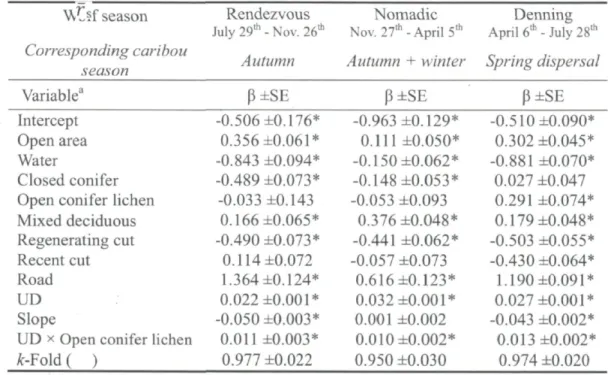
Table 2 Coefficients (P) and standard errors (SE) of mixed-effects logistic regression models of resource selection by gray wolves in managed boreal forests for three biological seasons of the year. The model accounts for multiple landscape features, as well as for changes in the selection of open conifer stands with lichen as a function of the wolf utilization distributions (UD). The /(-fold average values [rs values ± SE) for the cross validation are also reported.
W^ff season Rendezvous July 29th - Nov. 26th Corresponding caribou season Nomadic Nov. 27,h - April 5th Denning April 6th - July 28th
Autumn Autumn + winter Spring dispersal
Variable3 p±SE P±SE P±SE
Intercept Open area Water
Closed conifer Open conifer lichen Mixed deciduous Regenerating cut Recent cut Road UD Slope
UD x Open conifer lichen A:-Fold ( ) -0.506 ±0.176* 0.356 ±0.061* -0.843 ±0.094* -0.489 ±0.073* -0.033 ±0.143 0.166 ±0.065* -0.490 ±0.073* 0.114 ±0.072 1.364 ±0.124* 0.022 ±0.001* -0.050 ±0.003* 0.011 ±0.003* 0.977 ±0.022 -0.963 ±0.129* 0.111 ±0.050* -0.150 ±0.062* -0.148 ±0.053* -0.053 ±0.093 0.376 ±0.048* -0.441 ±0.062* -0.057 ±0.073 0.616 ±0.123* 0.032 ±0.001* 0.001 ±0.002 0.010 ±0.002* 0.950 ±0.030 -0.510 ±0.090* 0.302 ±0.045* -0.881 ±0.070* 0.027 ±0.047 0.291 ±0.074* 0.179 ±0.048* -0.503 ±0.055* -0.430 ±0.064* 1.190 ±0.091* 0.027 ±0.001* -0.043 ±0.002* 0.013 ±0.002* 0.974 ±0.020 aStands of open conifer without lichen were used as the reference category *95% confidence intervals exclude zero
A)Rendezvous 10 20 30 40 50 WolfUD CI Denning 0 10 20 30 40 50 60 70 80 WolfUD 0.0 J 0 10 20 30 40 50 60 70 WolfUD
Open conifer without lichen Open area
Water
Closed conifer Mixed deciduous Road
Open conifer lichen Regenerating cut Recent cut Mean Wolf UD Median WolfUD
Figure 2: Relative probability of occurrence for various land cover types as a function of the wolf utilization distribution (UD) in the boreal forest of Quebec (Canada), during: A) the rendezvous, B) nomadic, and C) denning seasons.
Movements of caribou
A total of 14,088 steps from 31 caribou were observed in areas occupied by the radio-collared wolves. During autumn, winter and spring dispersal, caribou adjusted their movements to multiple habitat attributes. They avoided steep slope areas, as well as water bodies, closed conifer stands, mixed and deciduous stands (all relative to
open conifer stands without lichen, Table 3). During autumn and winter, caribou also avoided regenerating cuts. In winter, they displayed such broad-scale avoidance of regenerating cuts that this land cover type was never available among observed or random steps and, therefore, could not be included in the winter SSF.
Table 3 Coefficients (P) and robust standard errors (SE) for step selection functions of forest-dwelling caribou in managed boreal forests for three biological seasons. Wolf utilization distributions (UD) were obtained using kernel methods whereas the wolf resource selection function (Wolf RSF, Table 2) was obtained using a generalized linear mixed model. A 3-knot linear spline function of distance moved has been added to the model. The /(-fold values (*% values ± SE) for the cross validation are also reported.
Caribou season Autumn Winter Spring dispersal
Oct. 13th -Dec 27th Dec. 28th-Apr 17th Apr 18th- May 27th
Variable3 P±SE P±SE P±SE
Open area 0.054 ±0.112 0.455 ±0.101* 0.354 ±0.068* Water -0.832 ± 0.234* -0.476 ± 0.224* -0.524 ±0.139* Closed conifer -0.323 ± 0.075* -0.195 ± 0.064* -0.168 ± 0.061* Open conifer lichen 0.526 ±0.064* 0.486 ±0.050* 0.660 ±0.074* Mixed deciduous -0.144 ± 0.084+ -0.151 ± 0.071* -0.168 ± 0.073* Regenerating cut -2.021 ± 0.807* 0.319 ±0.105* Recent cut 0.267 ± 0.547 -0.953 ± 0.396* 0.176 ±0.080* Road -0.072 ±0.105 Slope -0.045 ± 0.009* -0.030 ± 0.007* -0.018 ± 0.006* Road density -1.354 ± 0.598* -3.590 ± 0.998* -0.115 ±0.088 Wolf RSF -0.015 ±0.009+ 0.000 ± 0.007 -0.012 ± 0.004* UD -0.010 ±0.036 -0.028 ±0.022 -0.033 ± 0.017+ UD x Open conifer lichen -0.003 ± 0.004 0.008 ± 0.003* -0.024 ± 0.006* UD x Regenerating cut 0.017 ± 0.031 -0.007 ± 0.008 UDx Recent cut -0.022 ±0.021 0.085 ±0.033* 0.026 ±0.014+ UD x Road density 0.006 ±0.031 -0.012 ±0.058 0.004 ±0.006 Splinel 0.002 ±0.002 0.003 ±0.003 0.002 ±0.001 Spline2 0.002 ± 0.003 0.002 ± 0.004 -0.001 ±0.002 Spline3 -0.006 ± 0.001* -0.008 ± 0.002* -0.002 ± 0.001+ Spline4 _ 0.003 ± 0.000* 0.004 ± 0.000* 0.003 ± 0.000* k-Fo\d ( rs) 0.850 ±0.080 0.860 ±0.080 0.860 ± 0.080 aStands of open conifer without lichen were used as the reference category *95% confidence intervals exclude zero;
+90% confidence intervals exclude zero
The movement tactics of caribou varied between high use and low wolf-use areas (Table 3). During winter and spring dispersal, caribou were more likely to end their steps in open conifer stands with lichen than in any other land cover type when they traveled in areas of low wolf use (Table 3, Fig. 3). This selection for food rich patches was overall the most frequent response of caribou, as 1) this response was still observed for the median value of wolf UD and slightly above (see vertical dotted line in Fig. 3), hence over most of the landscape, and 2) the probability of occurrence of caribou was higher in areas of low wolf UD (Fig. 3). As wolf UD further increased from the median value, we observed a gradual shift in selection. Ultimately in high wolf-use areas, caribou became less likely to end their steps in open conifer stands with lichen than in recent cuts during winter and spring dispersal (Fig.3). We did not detect any changes in the selection of open conifer with lichen following changes in wolf UD in autumn (Table 3), and the movement of caribou remained strongly biased towards open conifer with lichen (Fig. 3A).
0.0 J
20 30
WolfUD
30 40 50 WolfUD
Open conifer without lichen Open area
Water
Closed conifer Mixed deciduous Road
Open conifer lichen Renegerating cut Recent cut Road density Mean WolfUD Median WolfUD
Figure 3: Relative probability that caribou select steps ending in various land cover types as a function of the wolf utilization distribution (UD) along the steps of caribou observed in the boreal forest of Quebec (Canada), during: A) the autumn, B) winter, and C) spring dispersal seasons.
V. Discussion
Our study has shown that caribou alter their movements in response to the spatial distribution of wolves and, most commonly, caribou won the behavioral response race. The spatial game between wolves and caribou generally displayed attributes of leapfrog effects, with the intensity of those effects varying over space and time. We thus provide one of the few empirical demonstrations of spatially structured leapfrog effects in animals ranging freely in their natural environments.
The distribution of prey commonly results from movement decisions balancing net energy gains and prédation risk (Linnell and Strand 2000, Lima 2002, Bell et al. 2009, Valeix et al. 2009). In a behavioral response race, predators can also adjust their distribution to various habitat attributes, resulting in a highly dynamic game with their prey (Lima 2002, Sih 2005, Dupuch et al. 2009, Laundré 2010, Williams and Flaxman 2012). Most models of predator-prey spatial games predict a positive association between the two groups (Sih 2005, Bell et al. 2009). We observed this during spring dispersal, where we found a positive relationship between the probability of occurrence of caribou and the intensity of wolf UD. Wolves thus appear to be winning the spatial game during this season, which could explain why 56% of caribou mortalities occur during spring dispersal (Courtois et al. 2007). This pattern of co-occurrence was not observed in the other studied seasons. During autumn and winter, we found a negative relationship between the probability of occurrence of caribou and the utilization distribution of wolves, thereby revealing that caribou were generally ahead of wolves in their behavioral race in those seasons.
A key factor determining the winner of the game is the relative strength of spatial anchors and constraints of predators and prey (Sih 2005). Evolutionary Stable Strategies tend to favor the player faced with the least constraining spatial anchors (Hammond et al. 2012). Wolves tend to focus their search on moose - their primary prey in the boreal forest (Messier 1994) - rather than on caribou (Basille et al. 2012,
but see Tremblay-Gendron 2012). Unlike caribou, moose select mixed and deciduous stands (Dussault et al. 2005), which become spatial anchors for wolves that require the predator to spend time away from areas preferred by caribou (e.g., open conifer stands with lichen). These differences in selection could partly explain a negative spatial association between wolves and caribou. Thus, food web complexity may give some advantage in the spatial game to secondary prey species by allowing them to avoid some of the predators' spatial anchors.
Nevertheless, caribou ultimately had to reduce their selection of food-rich areas and leave them to the wolves in order to win the game (Fig. 3). This is because during all three biological seasons that we investigated, wolves selected open conifer stands with lichen more strongly in sectors where they tended to focus their activities (i.e., high UD). This selection by the predator can be an adaptive response to an elusive prey: selecting static patches of its prey's resource may be less costly than trying to track mobile prey when predators only have limited information about prey's locations (Flaxman and Lou 2009). Although this tactic resulted in a positive spatial association with caribou during spring dispersal, we found a strong negative spatial association during autumn and winter. Denning season is when wolves select lichen-rich stands the most strongly; it is also when caribou displayed the strongest avoidance for those stands in areas where wolves focused their activities. The concurrent behavioral response of wolves and caribou to one another thus resulted in a leapfrog effect, with predators selecting their prey's high-quality food patches, while driving prey to undermatch their food resources (Sih 2005, Flaxman and Lou 2009).
Although caribou were generally able to win the spatial game, we observed strong spatial structure in the intensity of the leapfrog effect. Caribou selected forest stands providing the most lichen in areas of low wolf use (Fig 3), a search for food-rich patches generally expected by prey when predators are absent (Sih 2005, Hammond et al. 2007, Williams and Flaxman 2012); however, the cost-benefit balance seems to
tilt in areas of high wolf use, as caribou avoided stands rich in lichen. The marginal fitness gain of avoiding food-rich patches is known to strongly depend on the mortality risk of spending time in those patches (Brown et al. 1999), a risk that should be relatively high in areas with high predator densities. Accordingly, we only observed strong leapfrog effects in areas of high wolf activity.
Interestingly, caribou avoided lichen-rich areas in favor of recently cut forest stands when they were in high wolf-use areas. This response might be due to the strong avoidance of recent cuts by wolves during the denning season. While being slightly higher during the rendezvous season than in other seasons, the affinity of wolves for recent cuts never became strong - an observation that supports the findings of previous research (Lesmerises et al. 2012). Anthropogenic disturbances can thus serve as spatial refuges for prey during winter and spring dispersal (Basille et al. 2009, Hebblewhite and Merrill 2009, Muhly et al. 2011) and create an opportunity for prey to win the spatial game. However, not all anthropogenic disturbances that create spatial constraints for predators were used as refuges by caribou. Although regenerating cuts were avoided by wolves during denning and rendezvous season, they were also avoided by caribou in areas of high wolf use (Fig. 3).
In conclusion, our study demonstrates the behavioral response race between predator and prey in natural settings can be spatially structured. Empirical investigations reported strong variations - from negative to positive associations - in the spatial relationships between predators and prey (Rose and Leggett 1990, Fauchald et al. 2000, Mao et al. 2005, Laundré 2010, Hammond et al. 2012). Our study demonstrates that such variations can be observed over space and time, even within a single predator-prey system. By adjusting their movement and habitat selection in response to predator presence, caribou appear to be able to spatially and temporally moderate their prédation risk. Spatial relationships between predators and prey can
have a strong impact on species co-existence and population dynamics (Bell et al. 2009). Understanding the complex constraints on the behaviors of predators and prey can have important population and community-level implications (Hammond et al. 2012). For example, predators may force prey out of the richest patches, as observed in our study, thereby reducing the amount of food that is truly available to prey. Predicting how these interactions play out can provide critical information for the management and conservation of threatened prey populations, such as forest-dwelling woodland caribou, especially for populations that are faced with strong top-down forces.
VI. Acknowledgements
We thank The Fonds québécois de la recherche sur la nature et les technologies, the NSERC—University Laval industrial research chair in silviculture and wildlife, Université Laval, the Ministère des Ressources naturelles et de la Faune, Université du Québec à Rimouski, and the Canadian Foundation for Innovation for their financial support. We also thank P. Racine for his help with PostGIS, J.-P. Ouellet for his contribution to the project development, and B. Baillargeon, L. Breton, S. Couturier, D. Guay, D. Grenier, J.-Y. Laçasse and B. Rochette for their help in the field.
VII. References
Abramsky, Z., M. L. Rosenzweig, and A. Subach. 2002. The costs of apprehensive foraging. Ecology 83:1330-1340.
Basille, M., R. Courtois, G. Bastille-Rousseau, N. Courbin, G. Faille, C. Dussault, J.-P. Ouellet, and D. Fortin. 2010. Effets directs et indirects de l'aménagement de la forêt boréale sur le caribou forestier au Québec. Le Naturaliste Canadien 135:46-52.
Basille, M., D. Fortin, C. Dussault, J.-P. Ouellet, and R. Courtois. 2012. Ecologically based definition of seasons clarifies predator-prey interactions. Ecography in press. Basille, M., I. Herfindal, H. Santin-Janin, J. D. C. Linnell, J. Odden, R. Andersen, K. A.
Hogda, and J. M. Gaillard. 2009. What shapes Eurasian lynx distribution in human dominated landscapes: Selecting prey or avoiding people? Ecography 32:683-691.
Bates, D. and D. Sarkar. 2006. Linear mixed-effects models using S4 classes. R Package version 0.999375-32.
Batschelet, E. 1981. Circular statistics in biology. Academic Press, London, UK.
Bell, A. V., R. B. Rader, S. L. Peck, and A. Sih. 2009. The positive effects of negative interactions: Can avoidance of competitors or predators increase resource sampling by prey? Theoretical Population Biology 76:52-58.
Berger, J. 2007. Fear, human shields and the redistribution of prey and predators in protected areas. Biology Letters 3:620-623.
Beschta, R. L. and W. J. Ripple. 2010. Recovering riparian plant communities with wolves in Northern Yellowstone, USA. Restoration Ecology 18:380-389.
Beyer, H. L. 2009. Geospatial Modelling Environment (Version 0.3.3 Beta). (Software). URL: http://www.spatiaIecology.com/gme
Boyce, M. S. 2006. Scale for resource selection functions. Diversity and Distributions 12:269-276.
Boyce, M. S., P. R. Vernier, S. E. Nielsen, and F. K. A. Schmiegelow. 2002. Evaluating resource selection functions. Ecological Modelling 157:281-300.
Brown, J. S., J. W. Laundre, and M. Gurung. 1999. The ecology of fear: Optimal foraging, game theory, and trophic interactions. Journal of Mammalogy 80:385-399. Calenge, C. 2006. The package "adehabitat" for the R software: a tool for the analysis
of space and habitat use by animals. Ecological Modelling 197:516-519.
COSEWIC. 2002. COSEWIC assessment and update status report on the woodland caribou Rangifer tarandus caribou in Canada. Committee on the Status of Endangered Wildlife in Canada. Ottawa. 1-98 pp.
Courbin, N., D. Fortin, C. Dussault, and R. Courtois. 2009. Landscape management for woodland caribou: the protection of forest blocks influences wolf-caribou co-occurrence. Landscape Ecology 24:1375-1388.
Courtois, R., J.-P. Ouellet, L. Breton, A. Gingras, and C. Dussault. 2007. Effects of forest disturbance on density, space use, and mortality of woodland caribou. Ecoscience 14:491-498.
Cox, D. R. 1972. Regression models in life-tables. Journal of the Royal Statistical Society. Série B (Methodological) 34:187-220.
Craiu, R. V., T. Duchesne, and D. Fortin. 2008. Inference methods for the conditional logistic regression model with longitudinal data. Biometrical Journal 50:109-109.
Creel, S., J. Winnie, B. Maxwell, K. Hamlin, and M. Creel. 2005. Elk alter habitat selection as an antipredator response to wolves. Ecology 86:3387-3397.
Crête, M. and R. Courtois. 1997. Limiting factors might obscure population regulation of moose (Cervidae: Alces alces) in unproductive boreal forests. Journal of Zoology 242:765-781.
Crête, M., C. Morneau, and R. Nault. 1990. Biomasse et espèces de lichens terrestres disponibles pour le caribou dans le nord du Québec. Canadian Journal of Botany 68:2047-2053.
Dupuch, A., L. M. Dill, and P. Magnan. 2009. Testing the effects of resource distribution and inherent habitat riskiness on simultaneous habitat selection by predators and prey. Animal Behaviour 78:705-713.