Improved simulation of river water and groundwater exchange in an alluvial plain using the SWAT model

O

pen

A

rchive

T

OULOUSE

A

rchive

O

uverte (

OATAO

)

OATAO is an open access repository that collects the work of Toulouse researchers and

makes it freely available over the web where possible.

This is an author-deposited version published in :

http://oatao.univ-toulouse.fr/

Eprints ID : 15831

To link to this article : DOI :10.1002/hyp.10575

URL :

http://dx.doi.org/10.1002/hyp.10575

To cite this version : Sun, Xiaoling and Bernard-Jannin, Léonard and

Garneau, Cyril and Volk, Martin and Arnold, Jeffrey G and Srinivasan,

Raghavan and Sauvage, Sabine and Sanchez-Pérez, José-Miguel

Improved simulation of river water and groundwater exchange in an

alluvial plain using the SWAT model. (2015) Hydrological Processes,

vol. 30 (n° 2). pp. 187-202. ISSN 0885-6087

Any correspondance concerning this service should be sent to the repository

administrator:

staff-oatao@listes-diff.inp-toulouse.fr

Improved simulation of river water and groundwater exchange

in an alluvial plain using the SWAT model

X. Sun,

L. Bernard-Jannin,

C. Garneau,

M. Volk,

J. G. Arnold,

R. Srinivasan,

S. Sauvage

and J. M. Sánchez-Pérez

*

1

INPT, UPS; Laboratoire Ecologie Fonctionnelle et Environnement (EcoLab), University of Toulouse, Avenue de l’Agrobiopole, Castanet Tolosan, Cedex, 31326, France

2_{EcoLab, CNRS, Castanet Tolosan, Cedex, 31326, France} 3

Department of Computational Landscape Ecology, UFZ Helmholtz Centre for Environmental Research, Permoserstr. 15, Leipzig D-04318, Germany

4

Grassland, Soil & Water Research Laboratory, USDA-ARS, Temple, TX, 76502, USA

5

Spatial Science Laboratory in the Department of Ecosystem Science and Management, Texas A&M University, College Station, TX, 77845, USA

Abstract:

Hydrological interaction between surface and subsurface water systems has a significant impact on water quality, ecosystems and biogeochemistry cycling of both systems. Distributed models have been developed to simulate this function, but they require detailed spatial inputs and extensive computation time. The soil and water assessment tool (SWAT) model is a semi-distributed model that has been successfully applied around the world. However, it has not been able to simulate the two-way exchanges between surface water and groundwater. In this study, the SWAT-landscape unit (LU) model – based on a catena method that routes flow across three LUs (the divide, the hillslope and the valley) – was modified and applied in the floodplain of the Garonne River. The modified model was called SWAT-LUD. Darcy’s equation was applied to simulate groundwater flow. The algorithm for surface water-level simulation during flooding periods was modified, and the influence of flooding on groundwater levels was added to the model. Chloride was chosen as a conservative tracer to test simulated water exchanges. The simulated water exchange quantity from SWAT-LUD was compared with the output of a two-dimensional distributed model, surface–subsurface water exchange model. The results showed that simulated groundwater levels in the LU adjoining the river matched the observed data very well. Additionally, SWAT-LUD model was able to reflect the actual water exchange between the river and the aquifer. It showed that river water discharge has a significant influence on the surface–groundwater exchanges. The main water flow direction in the river/groundwater interface was from groundwater to river; water that flowed in this direction accounted for 65%of the total exchanged water volume. The water mixing occurs mainly during high hydraulic periods. Flooded water was important for the surface–subsurface water exchange process; it accounted for 69% of total water that flowed from the river to the aquifer. The new module also provides the option of simulating pollution transfer occurring at the river/groundwater interface at the catchment scale.

KEY WORDS SWAT model; landscape unit; water exchange; floodplain; Garonne River

INTRODUCTION

In recent decades, numerous studies have been carried out on the hydrological linkage between surface and subsurface water (SW–GW) systems (Grannemann and Sharp, 1979; Harvey and Bencala, 1993; Wroblicky et al., 1998; Malard et al., 2002). One of the most promising linkage concepts has been the development of what is known as the hyporheic zone. It was first presented by

Orghidan (1959) as a special underground ecosystem, but numerous different definitions by ecologists, hydrologists and biogeochemists have since been proposed (Sophocleous, 2002; Hancock et al., 2005). In all the definitions, the most important characteristic of hyporheic zones is the area of mixing between surface and subsurface water (White, 1993; Wondzell, 2011). As surface water contains rich oxygen and organic matter, and groundwater contains abundant nutriment elements, the water mix between those two systems has a significant impact on water quality, ecosystems and biogeochemistry cycling (Brunke and Gonser, 1997; Boulton et al., 1998; Sánchez-Pérez and Trémolières, 2003; Vervier et al., 2009; Krause et al., 2013; Marmonier et al., 2012).

The processes occurring at the river/groundwater interface are particularly important for the alluvial plains.

*Correspondence to: J. M. Sánchez-Pérez, Laboratoire d’Ecologie Fonctionnelle et Environnement (ECOLAB), UMR 5245 CNRS-UPS-INPT Ecole Nationale Supérieure Agronomique de Toulouse (ENSAT), Avenue de l’Agrobiopole BP 32607, Auzeville Tolosane, Castanet Tolosan, Cedex 31326, France.

One of the important features of the alluvial plains is deposited sediment. Their depositional structure leads to higher hydraulic conductivity in the aquifer region than in adjacent upland (Woessner, 2000). As they support important agricultural activities, groundwater in alluvial plains often suffers from nitrate pollution (Arrate et al., 1997; Sánchez-Pérez et al., 2003a; Liu et al., 2005; Almasri and Kaluarachchi, 2007). Several studies show that the surface–groundwater interface contributes to nitrogen retention and/or transformation of the land-surface water continuum (Sabater et al., 2003; Weng et al., 2003). This interface supports the purification of water by its ability to eliminate nitrates during their infiltration through the vegetation–soil system to ground-water, and also through diffusion from groundwater to surface water (Sanchez-Perez et al., 1991a,b; Takatert et al., 1999) Hence, an understanding of the processes occurring in the surface–groundwater interface could offer considerable insight for the purposes of water management on a catchment scale.

SW–GW interactions are complex processes driven by geomorphology, hydrogeology and climate conditions (Sophocleous, 2002). In addition, it has been stated that overbank flow is a key hydrological process affecting riparian water table dynamics and ecological processes (Naiman and Decamps, 1997; Rassam and Werner, 2008). Models have been developed to simulate the hydrological conditions of the surface water, groundwater and river/groundwater interface. Rassam and Werner (2008) reviewed models at different complex levels that represented the surface and subsurface processes that have influence on the SW–GW exchange. The simulation of the SW–GW exchange is mainly carried out by using three types of models: (i) models developed for subsurface water, (ii) models developed for surface water and (iii) models that integrated the interface of the two domains. To account for complex geometry, hydrological conditions and materials composition, most of the models developed for subsurface water are distributed models, such as MODFLOW (Storey et al., 2003; Lautz and Siegel, 2006) or HYDRUS (Langergraber and Šimůnek, 2005). These models usually require spatial inputs in high resolution and numerous parameters and are characterized by a significant computation time that inhibits their application on large scales. Models that are developed for surface water include QUAL2K (Park and Lee, 2002) and OTIS (Morrice et al., 1997). In these models, the lateral floodplain operates as a storage pool to keep the upstream and downstream channel water balance. Loague and VanderKwaak (2004) and Kollet and Maxwell (2006) reviewed models that coupled surface and subsurface domains, and FSTREAM (Hussein and Schwartz, 2003) and surface–subsurface water exchange model (2SWEM) (Peyrard et al., 2008) are examples for this type of model.

Most of these models are still too complicated to apply at a large scale.

Large-scale hydrological models have been developed to simulate hydrological conditions at a catchment or regional scale. Examples of such models include SWIM (Krysanova et al., 1998), TOPMODEL (Franchini et al., 1996) and MODHYDROLOG (Chiew and McMahon, 1994). However, the river/groundwater interface is mostly not included in these models. To overcome this issue, the incorporation of conceptual and distributed models has been suggested, as in SWAT-MODFLOW (Sophocleous and Perkins, 2000; Kim et al., 2008), WATLAC (Zhang and Li, 2009) and WASIM-ETH-I-MODFLOW (Krause and Bronstert, 2007). However, these developments have still been unable to reflect the impacts of land use management on groundwater quantity or are not applica-ble in large watersheds. The soil and water assessment tool (SWAT) model is a deterministic, continuous, semi-distributed, watershed-scale simulation model that allows a number of different physical processes to be simulated in a watershed. SWAT can simulate a large watershed with readily available data and has been used successfully all over the world (Jayakrishnan et al., 2005; Romanowicz et al., 2005; Fohrer et al., 2014). To reflect the hydrological connection between upslope and down-slope parts of a landscape, a catena approach including divide, hillslope and floodplain landscape units (LUs) has been developed and included in SWAT (Volk et al., 2007; Arnold et al., 2010; Rathjens et al., 2015). The catena approach in the modified model (SWAT-LU) represents an effort to impose a systematic upscaling from a topographic position to a watershed scale. Within the catena, a more detailed downslope routing of surface runoff, lateral flow and groundwater can be accomplished, and the impact of upslope management on downslope landscape positions can be assessed (Arnold et al., 2010; Bosch et al., 2010). However, the hydrological processes are still single tracks in SWAT-LU, and the function of SW–GW exchange in both directions is not included. Furthermore, the flooded distance during flooding events is fixed at five times the width of the top channel, and the influence of flooding on groundwater levels is not taken into account.

In this study, a new module was developed to simulate the SW–GW exchange in the river/groundwater interface. The modified model was called SWAT-LUD. The SWAT-LUD model was tested on the example of the floodplain of the Garonne River, which has a typical alluvial plain starting from its middle section. Several distributed models (MODFLOW, MARTHE and 2SWEM) were applied to simulate the hydrological and biogeochemical processes in this area (Sánchez-Pérez et al., 2003b; Weng et al., 2003; Peyrard et al., 2008). Groundwater levels and water exchanges between

SW–GW were simulated in the present study. The simulated groundwater levels were then compared with the groundwater levels measured by the piezometers, and the simulated water exchanges verified by detecting the concentration of conservative tracer and undertaking a comparison with the simulated results of a two-dimensional (2D) distributed model – 2SWEM.

METHODOLOGY SWAT model

The SWAT model (Arnold et al., 1998) is a semi-distributed, watershed-scale simulation model. It was developed to simulate the long-term impact of manage-ment on water, sedimanage-ment and agricultural chemical yields in large river basins. It is a continuous time model that is operating on a daily time step. To represent the spatial heterogeneity, the watershed is first divided into subba-sins. The subbasins are then subdivided into hydrological response units (HRUs), which are particular combinations of land cover, soil type and slope. SWAT is a process-based model; the major components include hydrology, nutrients, erosion and pesticides. In the SWAT model, processes are simulated for each HRU and then

aggregated in each subbasin by a weighted average (Arnold et al., 1998; Neitsch et al., 2009).

Model development

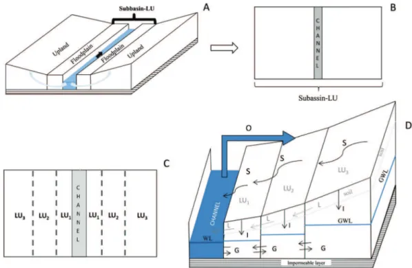
LU structure

.

usual SWAT model, flow is summed at the subbasin scale and not routed across the landscape. For this application, the watershed was divided into three LUs: the divide, the hillslope and the valley bottom. A representative catena was selected, and flow was routed across the catena as shown in Figure 1 (Volk et al., 2007). LUs represent additional units that take place between a subbasin and an HRU. Each subbasin is composed of three LUs, and HRUs are distributed across the different LUs (Volk et al., 2007; Arnold et al., 2010; Bosch et al., 2010; Rathjens et al., 2015). To represent the SW–GW exchanges occurring in the alluvial plain, a new type of subbasin called subbasin-LU was developed. Subbasin-LU corresponds to the subbasin delimited by the floodplain, and the LU structure was applied in subbasin-LU. Processes in the upland area of floodplain were calculated according to the original SWAT model. Processes were simulated for each HRU and aggregated to the river. Upland and subbasin-LU were connected through the river. The definition of the widths of LUs was made according to the surface of floodplain

Figure 1. The catena method and its landscape unit (LU) structure in the soil and water assessment tool (SWAT)-LUD model. The figure shows the location of subbasin-LU, the LU structure in the SWAT-LUD model and the hydrologic processes: ‘A’ represents the location of subbasin-LU, ‘B’ represents subbasin-LU, ‘C’ represents the distribution of LUs in the subbasin-LU (plane) and ‘D’ represents the hydrologic processes in the LUs, where ‘S’ is surface flow, ‘L’ is lateral flow, ‘I’ is infiltration, ‘G’ is groundwater flow, ‘O’ is overbank flow, ‘GWL’ is groundwater level and ‘WL’ is river

covered by the flood return period: LU1represented the

1-year return flood area, LU2 represented the 2- to 5-year

return flood area and LU3corresponded to the 10 or more

years’ return flood area. LUs were located parallel to the channel and were defined by their widths and slopes. As LUs were located on both sides of the channel, the width of each side of LU was half its total width. All three LUs in one subbasin were considered as being of the same length, which was the length of the channel. Processes in each HRU were still computed separately and then summed at LU scale. The length was defined based on the river’s hydromorphological structure. Finally, the processes were computed between LUs. With the catena method, surface runoff and lateral flow from LU3(which was furthest from

the channel) were routed through LU2to LU1(which was

nearest to the channel) and then entered the channel (Figure 1). A detailed description of the catena method can be found in Volk et al. (2007) and Arnold et al. (2010). SW–GW interaction with LU structure

.

equation (Equation (2.2.2.1)) was applied to calculate groundwater flow between the LUs and water exchanges between the river and the aquifer. Each LU had a unique groundwater level. The altitude of the riverbed in each subbasin was assumed to be the referenced value of the hydraulic head used to compute groundwater and surface water levels. HRUs were assumed to be homogenous inside, with no additional differentiation in soil and material underneath, and lateral flow was not simulated:

Q¼ K"A"ΔH

L (2:2:2:1) where Q is water flow (m3_day#1_{), A is the cross-sectional}

area between two units (m2_{), K is saturated hydraulic}

conductivity (m day#1), H is hydraulic head difference between two units (m) and L is the distance between two units through which the water is routed (m).

As the river is filled by water, two implementations of Darcy’s equation were required:

(1) Groundwater flow between two LUs: K ¼ðKlua"WluaÞ þ Kð lub"WlubÞ

Wluaþ Wlub

ð Þ (2:2:2:2) W¼ Wð luaþ WlubÞ=4 (2:2:2:3)

Q¼ 2"K"A"ðHlua# HlubÞ

W (2:2:2:4) where K represents the averaged hydraulic conductivity values of the two LUs (Klua, Klub) based on their widths

(m day#1), Wluaand Wlubare the widths of the two LUs

(m), Hluaand Hlubare the hydraulic heads of the two LUs

(m) and W is the distance between the centres of these two

LUs on one side of channel. Because LUs are located in two sides of the channel, each side obtained half of its width, and W is a quarter of the total width of these two LUs (m). As groundwater flow occurs on both sides of the river, the flow was multiplied by two.

(2) Groundwater flow between LU1and the river:

K¼ Klu (2:2:2:5)

W ¼ Wð luÞ=4 (2:2:2:6)

Q¼ 2"K"A"ðHlu# HchÞ

W (2:2:2:7) where K is the hydraulic conductivity value of LU1(Klu)

(m day#1); W is the quarter width of LU1(Wlu) (half of the

width of one side of the channel) (m); and Hluand Hchare

hydraulic heads of LU1and the river (m).

Influence of flooding to surface water and groundwater level

.

SWAT model only assumes that the flooded distance is five times the top channel width (Neitsch et al., 2009). The influence of floodplain geometry and the influence of flooded water on groundwater are not considered. The new algorithm was based on the water volume during a flood event:

Uf ¼ v # vð maxÞ"T (2:2:3:1)

where Uf is the flood volume (m3), v is the discharge

(m3s#1), vmax is the maximum discharge value at which

water could stay in the channel (m3s#1) and T is the travel time of water passing through the channel (s).

During a flood, the surface water level is the sum of the riverbank height and the water depth on the surface relative to the height of riverbank:

Af ¼ Lch' Wchþ Lf ! " (2:2:3:2) Hch¼ Dchþ Uf Af (2:2:3:3)

where Af is the flooded area (m2), Lchis the length of the

channel (m), Wchis the width of the channel (m), Lfis the flood

distance on one side of the riverbank (m), Hchis the surface

water level and Dchis the height of the riverbank (m).

With regard to groundwater levels in the LUs during flood periods (if flood water arrives at a LU), the groundwater of this LU was assumed to be the same level as the surface water:

Hluf ¼ Hch (2:2:3:4)

where Hluf is the groundwater level of LU during the

The infiltrated flood water was calculated as follows: Vin;f ¼ Hluf # Hlu

!

""Alu"plu (2:2:3:5)

where Vin,f is the infiltrated flood water volume in LU

(m3_{), A}

luis the surface area of the LU (m2) and pluis the

porosity of the LU (%).

The overbank flow would return back to the river the next day after flooding, and discharge of river water was recalculated:

IN ¼ IN þ Uf (2:2:3:6)

v¼ IN=86 400 (2:2:3:7) where IN is the input water volume (m3₎

Transfer of dissolved elements

.

dis-solved elements between LUs and between LUs and surface water was calculated based on the water flow volume and concentration of the elements:

Mlu¼ Mluþ Min# Mout (2:2:4:1)

Min¼∑ Vð in'CinÞ (2:2:4:2)

Mout¼∑ Vð out'CluÞ (2:2:4:3)

Clu ¼ Mlu=Vlu (2:2:4:4)

where Mluis the mass content of the element in LU (g),

Minis the input mass (g) and Moutis the output mass (g).

Vinis input water volume (m3), Cinis the concentration of

the elements in the input water (mg l#1), Voutis the output

volume (m3), Clu is the concentration of the element in

calculated LU (mg l#1) and Vlu is the water volume

storage in LU (m3). Study area

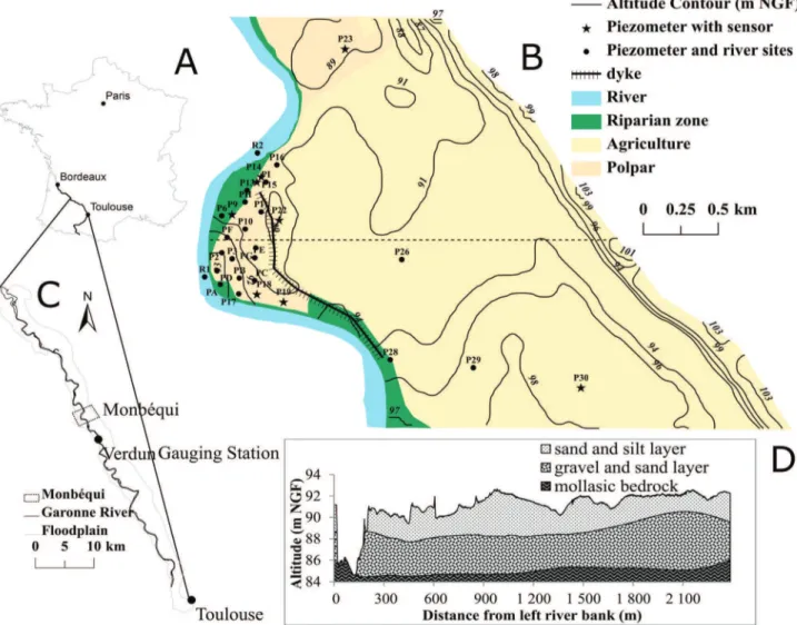
The Garonne River is the third longest river in France. Its hydrology is influenced by Mediterranean climate and melting snow from the mountainous areas. The typical alluvial plain starts from the middle section of the Garonne River. It contains between 4- and 7-m coarse deposits (quaternary sand and gravel) eroded from the Pyrenees Mountains during the past glacial periods that overlie the impermeable layer of molassic substratum (Lancaster, 2005). The Verdun gauging station is located at about 4 km upstream of the study site Monbéqui. It is the nearest gauging station to the study site at the Garonne River. At the Verdun gauging station, the Garonne has a watershed size of 13 730 km2and an annual average flow of about 200 m3s#1. The monthly average flow ranges from about 75 m3s#1 in August to about 340 m3s#1 in May (Banque Hydro, http://www.hydro.eaufrance.fr/).

The greatest discharges occur twice a year, in the spring as a result of snow melt and in late autumn following intense rainfalls (Sánchez-Pérez et al., 2003c). Previous studies in the Garonne river basin have shown that the river/groundwater interface plays an important role at the reach scale, both in the retention of nitrogen and phosphorous (Vervier et al., 2009) and in controlling aquifer water quality (Iribar et al., 2008). The study area is characterized by high nitrate pollution caused by agriculture (Jégo et al., 2008, 2012).

The study site is located in a meander of the alluvial plain of the Garonne River (Monbéqui), and the width of the floodplain in the area is about 4 km. The mean annual precipitation is about 690 mm in this area. The alluvium thickness ranges from 2.5 to 7.5 m, with an arithmetic mean of 5.7 m (Sánchez-Pérez et al., 2003c). The groundwater table varies from 2 to 5 m in low water periods and rises rapidly up to soil profile during floods (Weng et al., 2003). The first 50–200 m of the riverbank is covered by riparian forest and poplar plantations, surrounded by agricultural land. Several terraces exist in this area, generated by sediment deposition and washing out by flooding events. Artificial dykes have been constructed in the region to protect the agricultural land (Figure 2).

Measurements

.

in the study area, nine of which were equipped with water-level sensors [Orphimedes, OTT (in 1999–2000) and CTD-diver, Schlumberger, Germany (in 2013)] to record changes in groundwater level every 10 min. In addition, groundwater samples were taken monthly for analysis of physicochemical parameters. While pH, redox potential, electrical conductivity, oxygen content and temperature were measured in the field, other parameters such as nitrate, dissolved organic carbon and chloride were analysed in the laboratory.

In 1999–2000, the groundwater levels of six piezometers (P9, P15, P19, P22, P23 and P30) were recorded with water-level sensors, while groundwater samples were not taken; therefore, physicochemical parameters were not analysed during this period. In 2013, 25 piezometers (all the piezometers in Figure 2 except P15, P19, P23 and P29) and two river sites (R1 and R2) were sampled monthly, and groundwater-level sensors fitted in five piezometers (P7, P9, P14, P18 and P22). Piezometers that were recorded in both periods are P9, P22 and P30 (Figure 2).

LU parameters

For the purposes of simplification, only one subbasin-LU was simulated in this study, and each subbasin-LU only contained one HRU. The daily discharge data of the Verdun gauging station were used as input data. Based on the flooded area of the Garonne River during different

periods, the LU parameters are presented in Table I; the values of porosity were given based on the study of Seltz (2001) and Weng et al. (2003). The distributions of piezometers with installed sensors in the three LUs were as follows: five piezometers were located in LU1: P9,

P14, P15, P18 and P19; two piezometers, P22 and P23, were located in LU2; and P30 was located in LU3.

In the model, each LU had one groundwater-level value. With Darcy’s equation, the altitude of the riverbed in each subbasin-LU was assumed to be the referenced hydraulic head. As the river sloped, the altitude of the riverbank was variable within one subbasin-LU. One referenced value had to be chosen for comparison with the measured groundwater levels in each subbasin-LU. At the study site, P9 was the only piezometer with groundwater-level sensors fitted during 1999–2000 and 2013 in LU1. The

groundwater level of LU1 was more important to the

calculation of the SW–GW exchange than that of the other two LUs. The altitude of the riverbed was set at 84.75 m National Geographique Français (NGF: the general levelling of France, with ‘zero level’ determined by the tide gauge in Marseille). It was calculated based on the altitude of the soil surface of P9 (88.95 m NGF) minus 4 m, corresponding to the height of the riverbank minus 0.2 m and the slope of LU1that was 0.002.

Figure 2. The Garonne River and the Monbéqui study site. ‘A’ represents the location of the Garonne River, ‘B’ represents the location of the alluvial plain and Monbéqui, ‘C’ represents the piezometers in Monbéqui and ‘D’ represents the cross-section profile of the floodplain correspondence to the dash

line in ‘C’. NGF, National Geographique Français

Table I. Parameters of LUs and channel

LU1 LU2 LU3 Channel Width (km) 0.4 0.8 3.0 0.22 Length (km) 6.374 6.374 6.374 6.347 Slope (lateral) 0.002 0.005 0.005 — Slope (vertical) — — — 0.001 Porosity 0.1 0.1 0.1 — Depth (m) — — — 4.0

Calibration and validation

Groundwater levels

.

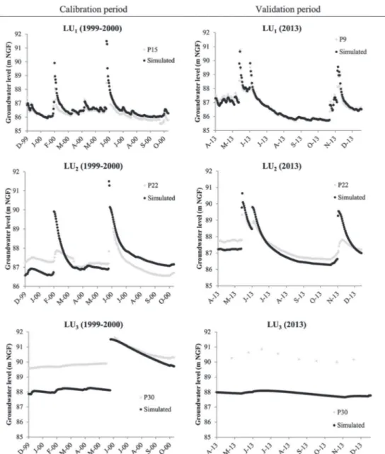
groundwa-ter levels was performed manually. Because the flood that occurred in 2000 was the largest event in the recent 20 years, and the groundwater-level sensors were installed in all the three LUs in the period of 1999–2000, the observed groundwater levels in this period were used as calibration data. The observed data from 2013 were taken as validation data. The simulated groundwater levels of the LUs (average value) were compared with correspond-ing piezometers (point value). To limit the error caused by the vertical slope, piezometers were chosen for compar-ison with the simulated groundwater levels in each LU based on their location relative to P9. In LU1, P15 and P9

had similar observed values in the calibration period (1999–2000), but P15 had a longer available time series than P9. In LU2, P22 was closer to P9 than P23. P30 was

located upstream of P9 but was the only piezometer with a groundwater-level sensor installed in LU3. Therefore,

the observed groundwater levels of P15, P22 and P30 during the calibration period (1999–2000) and P9, P22 and P30 during the validation period (2013) were used for comparison with the simulated results of LU1, LU2 and

LU3, respectively.

SW–GW exchanged water

.

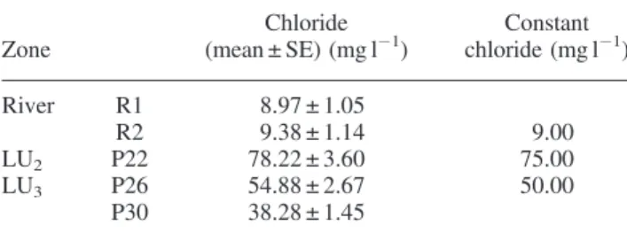
groundwater conservative tracer (Harvey et al., 1989; Cox et al., 2007) was chosen to verify the simulated water exchange between the river and LU1. Because the

concen-trations of chloride were measured monthly, there are a lack of continuous observed data as input values of the model. However, the variations of the chloride concentrations in surface water and groundwater in LU2as well as in LU3were

only slight; constant concentration values were given for the river, LU2and LU3during simulation. Concentration values

were set based on the measured data in 2013 (Table II), because this was the only year in which surface water and groundwater samples were taken and analysed. The concentration values in LU1 were simulated based on the

mix of surface water and LU2. The comparison of simulated

and observed chloride concentrations in LU1could be used to

verify the simulated SW–GW exchange in LU1.Because the

transport of chemistry elements was more complicated than water flow, it would be more difficult to match the simulated data for a LU with the observation from a certain piezometer. The chloride concentrations measured in all the 16 piezometers in LU1were compared with the simulated data.

Surface–subsurface water exchange model is a 2D hydraulic model. Horizontal 2D Saint Venant equations for river flow and a 2D Dupuit equation for aquifer flow were coupled in the model to simulate the dynamic variation of aquifer water level. It was originally developed to simulate water exchange occurring in the river/groundwater interface (Peyrard et al., 2008). Peyrard (2008) simulated surface water and groundwater exchange on the right side of the riverbank in the Monbéqui study area. The simulation was carried out for a 3.1-km length of the riverbank using the 2SWEM at a daily time step. The result of the SWAT-LUD simulation was adjusted [total exchanged volume divided by the length of channel (6.374 km) multiplied by 3.1 km] to match the distance of 3.1 km and then divided by 2 to compare it with the output of the 2SWEM.

The coefficient of determination (R2

), Nash–Sutcliffe efficiency (NSE), percent bias and root-mean-square error observations standard deviation ratio were chosen as evaluating parameters.

RESULTS Calibrated parameters

Hydraulic conductivities were determined by pumping tests and slug tests, varying from 10#2 to 10#5m s#1 (Weng et al., 2003; Peyrard et al., 2008). Because the simulations with the SWAT-LUD model were carried out at a daily step, the converted daily hydraulic conductiv-ities varied from 860 to 1 m day#1. Calibrated parameters are given in Table III.

Groundwater levels

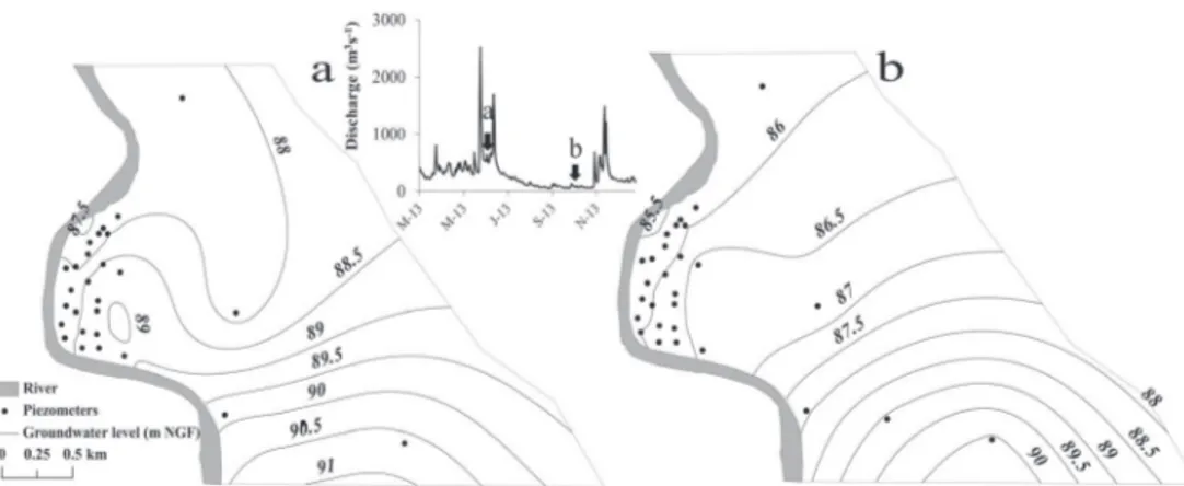
Figure 3 shows the shallow water tables in the study site based on the measured data of all the piezometers in two periods in 2013.

Table II. Detected values (in 2013) and constant values of chloride of river water and groundwater of LU3and LU2

Zone Chloride (mean ± SE) (mg l#1) Constant chloride (mg l#1) River R1 8.97 ± 1.05 R2 9.38 ± 1.14 9.00 LU2 P22 78.22 ± 3.60 75.00 LU3 P26 54.88 ± 2.67 50.00 P30 38.28 ± 1.45

LU, landscape unit; SE, standard error.

Table III. Manually calibrated parameters

Parameters

Default value

Calibrated values Manning roughness coefficient 0.014 0.070 Hydraulic conductivity (LU1) (m day#1) Undefined 300

Hydraulic conductivity (LU2) (m day#1) Undefined 200

Hydraulic conductivity (LU3) (m day#1) Undefined 100

It shows that in the period between two floods, the direction of groundwater flow in the meander is from river to floodplain, and groundwater flowed from the floodplain to river in the stable low flow period.

The comparison of observed and simulated groundwa-ter levels in the three LUs is shown in Figure 4.

The results demonstrated that observed and simulated values matched very well in LU1, especially in 2013

when simulated and observed values almost overlapped (R2= 0.96, NSE = 0.95). There was considerable variation in the observed and simulated well heights in LU2. The

lower water-level values of the simulations were under the observations, and LU2 was flooded too often

compared with the observed data. For LU3, the result

showed that simulated values were much lower than the observed data in LU3, but the two curves had the same

variation trend (R2= 0.94) (Table IV). The graph also showed that with an increase in distance from the river, there was a decrease in the fluctuation in groundwater. Water exchange between surface water and groundwater

Water exchange – verified with conservative elements

.

To verify simulated exchanged water, simulated concentra-tion values of chloride (Cl#) were compared with the mean values from the 16 piezometers. The simulated groundwater level in LU1was compared with P15 and P9, but only P9

was sampled in 2013. The detected values of Cl#of P9 were also compared with the simulated data (Figure 5).

Figure 5 shows large variations in observed values within LU1, matching the mean values more closely than P9.

Comparison with simulations by the 2SWEM

.

shows the comparison between the results of the SWAT-LUD model and the results of the 2SWEM. The models produced reasonably close results given the R2 of 0.62 and NSE of 0.51 (Figure 6). In the period before May 2005, SWAT-LUD predicted less surface water entering the aquifer than the 2SWEM, and the lag time of

groundwater flow to the river was greater in 2SWEM than in SWAT-LUD. After a large peak in May 2005, the results of the two models were almost identical.

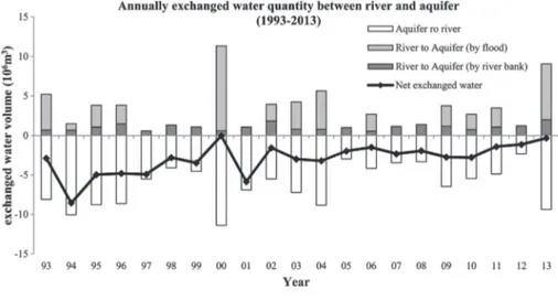
Surface water and groundwater exchange

.

quantity exchanged annually between the river and the aquifer throughout the entire period simulated (1993–2013) is shown in Figure 7. Water flow can occur in two directions: from the river to the aquifer and from the aquifer to the river. It was found that the dominant net flow direction was from the aquifer to the river and that water exchange quantities varied annually. Water flowing from the river to the aquifer can be separated into two parts: (1) water infiltrating through the riverbank and (2) flooded water percolating through the surface of the LUs. Flooded water percolating through the soil surface accounted for 69% of water flowed from the river to the aquifer. The annually flooded water volume and flooded days are shown in Figure 8.

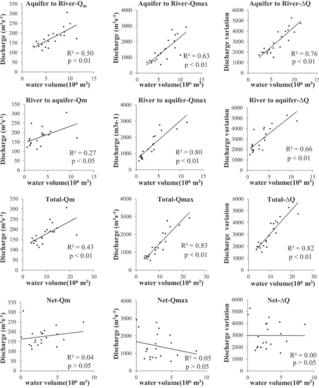
To understand the influence of river water discharge on the SW–GW exchanged water volumes, three river water discharge measurements were correlated with four simulated exchanged water volume components. The discharge measurements were annual mean discharge (Qm), annual maximum discharge (Qmax) and annual

discharge variation ΔQ ¼ ffiffiffiffiffiffiffiffiffiffiffiffiffiffiffiffiffiffiffiffiffiffiffiffiffiffiffi ∑ Q # Qð mÞ 2 q % & . The exchanged water volumes were the annual absolute exchanged water volume flowing in two directions (from river to aquifer and from aquifer to river), net exchanged water volume and total absolute exchanged volume. Results are shown in Figure 9. This demonstrated that river water discharge had a significant impact on the exchanged water quantities between the river and the aquifer. Along with the increase of Qm, Qmaxand∆Q, the

water volumes flowing from the river to the aquifer and from the aquifer to the river also increased. Water flow from the aquifer to the river is better correlated with∆Q. Qmax played the most significant role in water flowing

Figure 3. Contour maps of groundwater level in two periods: ‘a’ represents the groundwater levels in flood period and ‘b’ represents the groundwater levels in low hydraulic period. NGF, National Geographique Français

from the river to the aquifer and total exchanged water volume. However, net exchanged water volumes were not significantly influenced by the discharge.

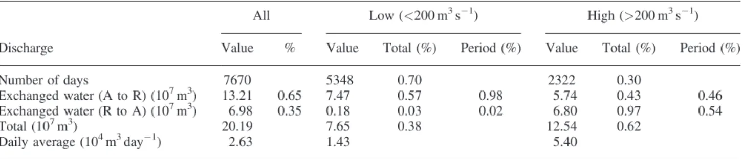
Based on the discharge values, simulated data were separated into two parts: low hydraulic period and high hydraulic period. The bound discharge value was set at 200 m3s#1, which is the long-term mean discharge of the Verdun gauging station (http://www.hydro.eaufrance.fr/). The results are given in Table V. During the entire simulation period, the water that flowed from the aquifer to the river accounted for 65% of the total exchanged water volume (exchanged water volume in two direc-tions). The low hydraulic period contributed 57% of the water that flowed from the aquifer to the river. The main water flow from the river to the aquifer occurred during the high hydraulic period, which amounted to 97% of the total flow in this direction.

In the low hydraulic period, the main water flow direction was from the aquifer to the river, which was

Figure 4. Observed and simulated groundwater levels in the calibration (1999–2000) and validation (2013) periods. LU, landscape unit; NGF, National Geographique Français

Table IV. Parameters for evaluating the accuracy of groundwater levels simulated by the SWAT-LUD model

R2 NSE PBIAS RSR LU1 Calibration 0.79 0.25 #0.27 0.87 Validation 0.96 0.95 #0.05 0.22 LU2 Calibration 0.38 #0.42 #0.15 1.19 Validation 0.78 0.48 0.09 0.72 LU3 Calibration 0.94 #4.14 1.12 2.27 Validation 0.75 #72.3 2.68 8.56

LU, landscape unit; NSE, Nash–Sutcliffe efficiency; PBIAS, percent bias; RSR, root-mean-square error observations standard deviation ratio; SWAT, soil and water assessment tool.

Figure 5. Comparison of concentration of chloride in LU1between the SWAT-LUD model’s simulation and values detected from field sampling in

2013. LU, landscape unit; SE, standard error; NSE, Nash–Sutcliffe efficiency; PBIAS, percent bias; RSR, root-mean-square error observations standard deviation ratio; SWAT, soil and water assessment tool

Figure 6. Comparison of the simulated water exchange between the SWAT-LUD model and the surface–subsurface water exchange model (2SWEM). NSE, Nash–Sutcliffe efficiency; PBIAS, percent bias; RSR, root-mean-square error observations standard deviation ratio; SWAT, soil and water

assessment tool

98% of the total water exchange in this period. The low flow period represented 70% of the simulated days, but the amount of exchanged water was only 38% of the total volume.

During the high hydraulic period, more water flowed from the river to the aquifer than from the aquifer to the river (54:46). However, the difference between those two flow directions was not as high as it was during the low flow period. The daily average flow in this period (5.40 × 104m3day#1) was much greater than during the low water period (1.43 × 104_m3_day#1_).

DISCUSSION

The SWAT-LU model was modified by adding in the floodplain area the module simulating SW–GW water exchange at the river/groundwater interface. The algo-rithms calculating surface water and groundwater levels during flooding were also modified in agreement with the module. The comparison of simulations and observations proved that the modified model was able to reflect accurately the actual hydrological dynamics in the aquifer of the floodplain of the Garonne River. Darcy’s equation was used to calculate water exchanges caused by the difference in hydraulic heads between the channel water and groundwater levels in LU1– hydraulic conductivities

are important parameters for calculating the SW–GW interaction (Sophocleous, 2002). The comparison of simulations and observed groundwater levels confirmed that the model can accurately simulate groundwater levels. Moreover, the simulated SW–GW exchange was verified by comparing it with the detected values of tracer from field samples and the simulated water exchange with a 2D distributed model: the 2SWEM. The results demonstrated that the SWAT-LUD model was able to simulate SW–GW water exchange accurately in terms of fluxes.

The model was able to reproduce the two-way interactions occurring in SW–GW exchanges. The contri-bution of surface water to subsurface flow is not considered in most of the existing catchment-scale models such as SWIM (Krysanova et al., 1998), TOPMODEL (Franchini et al., 1996) or MODHYDROLOG (Chiew and McMahon, 1994). However, the results from this study showed its importance, because it accounted for 35% of total SW–GW exchanges over a long period. The two-way interaction that controls water mixing in the river/groundwater interface is an important driver in biogeochemical reactions occurring in this area (Amoros and Bornette, 2002). The SWAT-LUD model presented here provides a solid basis for further model development aiming at the simulation of biogeochemical processes in floodplain areas at catchment scale.

Previous research and this study have proven that discharge in the channel is the main driving factor of the SW–GW exchange in the study site (Peyrard et al., 2008). As the main water flow direction during low hydraulic periods is from the aquifer to the river, the water mixing in river/groundwater interface occurs mainly during high hydraulic periods. Flooding has been proven to influence the plant communities of wetlands, in terms of both soil nitrate reduction and groundwater flow (Hughes, 1990; Casanova and Brock, 2000; Brettar et al., 2002; Alaoui-Sossé et al., 2005). In the present study, flooded water was found to be important for the SW–GW exchange process, which needs further investigation in future. As a daily step model, SWAT-LUD could not reflect the detailed processes occurring during flooding events. In this study, during flood periods, the groundwater levels of LUs reached by floodwater were considered to have the same value as the river water levels. The time lag of water infiltration was not taken into account, and as the LU has a unique groundwater level, the risk of overestimating infiltrated flooded water increased along with the increase

of the width of LUs. Because the surface area of LU3is

much larger than the two other LUs, if flooded water arrives in LU3, the infiltrated flooded water could be more

easily overestimated. The large flood that occurred during the calibration period reached LU3. This probably

explained the high simulated groundwater levels in LU2

and LU1 after the flooding event. The algorithm is still

simple, and the simulated exchanged water volume should be compared with the results of a distributed model or observed data in a future study.

The water loss caused by plant evapotranspiration, especially in the riparian forest zones, was stated in many

studies (Boronina et al., 2005; Butler et al., 2007; Gribovszki et al., 2008). However, because the ground-water table is usually beneath the root zone in the study site except during flood period, water uptake by plants is negligible and was not stated in this study. The influences of pumping on groundwater and river water flow were stated also in some researches (Hunt, 1999; Cooper et al., 2003; Rassam and Werner, 2008). This process was not included in the model yet, but it could be easily added to the model as an output source of groundwater in the future study. Because of the chosen model philosophy, the pumped water in each LU would be summed together, and influence of pumping on groundwater-level fluctuation would be simulated at LU scale (in contrast to more complex procedures in physically based models).

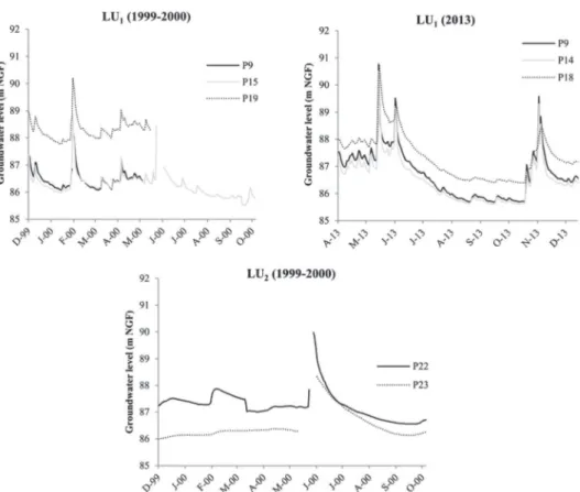
As a semi-distributed model, the SWAT-LUD model cannot consider detailed topographic information. In the model, each LU has a unique slope value and mean hydraulic conductivity. Because the model was applied at floodplain scale, the impermeable layer was considered to be flat in the model, and the complex topography of channel and adjacent floodplain was only considered to be mean slope for each LU. Channel processes and SW– GW water exchange were calculated at subbasin scale. Moreover, the groundwater was assumed to be flowing in a horizontal direction (perpendicular to the river flow). The vertical gradient of the groundwater hydraulic heads shown in Figure 10 was not considered. The existence of the vertical gradient was explained by the height difference between simulated groundwater levels and the observed values of P30 in LU3. In LU2, piezometer

P22 was located just behind an artificial dyke, which was built to protect agricultural land from flooding. Flooded water has to move to the top of the dyke before it arrives at P22. As the model could not consider this local detailed information, LU2 was oversaturated compared with the

observation from P22. In addition, the simulated groundwater levels represented the average situations of all the LUs, so it would be difficult for the output of the model to match data from one piezometer closely.

Moreover, hydraulic conductivity was a mean value in each LU. However, in reality, hydraulic conductivities are extremely heterogeneous (Weng et al., 2003), so the uncertainties of water-level simulations as a result of mean values linked to the mean values of hydraulic conductivities could be important when compared with local piezometers. To evaluate the uncertainties, a sensitivity analysis of hydraulic conductivity would be required.

The SWAT-LUD was not able to provide a detailed spatial distribution of hydraulic heads of the kind provided by physically based models [MODFLOW (Sánchez-Pérez et al., 2003b), MARTHE model (Weng et al., 2003) and 2SWEM (Peyrard et al., 2008)]. However, the objective of the study was not to provide accurate spatial representations of groundwater levels like the physically based models but to provide a good estimation of SW–GW interactions over a long timescale with a simple model. The model aimed to simulate large catchment sizes to support river basin water manage-ment. Therefore, the complexity of physically based models leading to long computation times for the simulation of small-scale areas (Helton et al., 2014; Lautz and Siegel, 2006) is not suitable. Moreover, physically based models need very detailed input information that can be difficult to collect, while this model needs only basic parameters. Nevertheless, SWAT-LUD gave similar results for SW–GW interac-tions when compared with the physically based 2SWEM (Peyrard et al., 2008). Although the shapes of the channels and LUs in the SWAT model were assumed to be straight and homogeneous, the values for exchanged water between river and aquifer simulated by the SWAT-LUD model were identical to the physically based 2SWEM. This showed that the SWAT-LUD model could accurately reflect the actual water exchange occurring at reach scale. SWAT-LUD was able to reproduce the spatial and temporal patterns of SW–GW exchanges at reach scale in a simple way, which means that it can be used for large catchment simulation and to support river basin management studies.

Table V. Simulated exchanged water quantity between river and aquifer in two hydraulic periods (low water period and high water period) throughout the simulated period (1993–2013)

Discharge

All Low (<200 m3

s#1) High (>200 m3

s#1) Value % Value Total (%) Period (%) Value Total (%) Period (%) Number of days 7670 5348 0.70 2322 0.30

Exchanged water (A to R) (107m3) 13.21 0.65 7.47 0.57 0.98 5.74 0.43 0.46 Exchanged water (R to A) (107m3) 6.98 0.35 0.18 0.03 0.02 6.80 0.97 0.54 Total (107m3) 20.19 7.65 0.38 12.54 0.62

Daily average (104m3day#1) 2.63 1.43 5.40

CONCLUSIONS

This paper has described the new module of the SWAT-LUD model created to simulate surface water and floodplain groundwater. Darcy’s equation was introduced to the model to simulate groundwater flow and SW–GW exchange occurring through the riverbank. The algo-rithms of river water and groundwater levels during flooding events were also modified. This new module was tested in a meander of the floodplain of the Garonne River in France. Comparisons between simulation results with observations from piezometers illustrated that the SWAT-LUD model could satisfactorily simulate groundwater levels near the area of the bank. Conservative tracer measured from field samples was used to validate the simulations, and SW–GW exchange modelling results with this approach corresponded well with the results obtained by a complex hydraulic model. This model was able to reflect accurately the actual water exchange between surface and subsurface systems of the alluvial plain of the Garonne River. River water discharge was found to have a great influence on the SW–GW exchange process. The main water flow direction was from groundwater to river; water that flowed in this direction in the river/groundwater interface accounted for 65% of the total exchanged water volume. The water mixing

occurs mainly during high hydraulic periods. Flooded water was important for the SW–GW exchange process; it accounted for 69% of total water flowed from the river to the aquifer. As a catchment-scale model, SWAT-LUD could easily be applied to a large catchment with basic available data. The SWAT-LUD model enabling simula-tion of GW–SW exchange processes at catchment scale would be a useful tool for evaluating the role of river buffer strips and wetlands in improving water quality. Future work should include (i) an application of the modified model in a larger catchment with multiple subbasins and (ii) the simulation of land management operations and biogeochemical processes in the river/groundwater interface.

ACKNOWLEDGEMENTS

We are grateful to N. B. Sammons for her help with developing the module. This study was performed as part of the EU Interreg SUDOE IVB programme (ATTENAGUA – SOE3/P2/F558 project, http://www. attenagua-sudoe.eu) and funded by ERDF. This research has been carried out as a part of ‘ADAPT’EAU’ (ANR-11-CEPL-008), a project supported by the French National Research Agency (ANR) within the framework of ‘The Global Environmental Changes and Societies

Figure 10. Observed groundwater levels in landscape units (LUs) with more than one piezometer equipped with a water-level sensor. NGF, National Geographique Français

(GEC&S) programme’. X. Sun is supported by a grant from the China Scholarship Council (CSC).

REFERENCES

Alaoui-Sossé B, Gérard B, Binet P, Toussaint M-L, Badot P-M. 2005. Influence of flooding on growth, nitrogen availability in soil, and nitrate reduction of young oak seedlings (Quercus robur L.). Annals of Forest Science 62: 593–600. DOI:10.1051/forest:2005052.

Almasri MN, Kaluarachchi JJ. 2007. Modeling nitrate contamination of groundwater in agricultural watersheds. Journal of Hydrology 343: 211–229. DOI:10.1016/j.jhydrol.2007.06.016.

Amoros C, Bornette G. 2002. Connectivity and biocomplexity in waterbodies of riverine floodplains. Freshwater Biology 47: 761–776. DOI:10.1046/j.1365-2427.2002.00905.x.

Arnold JG, Allen PM, Volk M, Williams JR, Bosch DD. 2010. Assessment of different representations of spatial variability on SWAT model performance. Transactions of the ASABE 53: 1433–1443.

Arnold JG, Srinivasan R, Muttiah RS, Williams JR. 1998. Large area hydrologic modeling and assessment part I: model development 1. JAWRA Journal of the American Water Resources Association 34: 73–89. DOI:10.1111/j.1752-1688.1998.tb05961.x.

Arrate I, Sanchez-Perez JM, Antiguedad I, Vallecillo MA, Iribar V, Ruiz M. 1997. Groundwater pollution in quaternary aquifer of Vitoria: Gasteiz (Basque Country, Spain): influence of agricultural activities and water-resource management. Environmental Geology 30: 257–265. DOI:10.1007/s002540050155.

Boronina A, Golubev S, Balderer W. 2005. Estimation of actual evapotranspiration from an alluvial aquifer of the Kouris catchment (Cyprus) using continuous streamflow records. Hydrological Processes 19: 4055–4068. DOI:10.1002/hyp.5871.

Bosch DD, Arnold JG, Volk M, Allen PM. 2010. Simulation of a low-gradient coastal plain watershed using the SWAT landscape model. Transactions of the ASABE 53: 1445–1456.

Boulton AJ, Findlay S, Marmonier P, Stanley EH, Valett HM. 1998. The functional significance of the hyporheic zone in streams and rivers. Annual Review of Ecology and Systematics 29: 59–81. DOI:10.1146/ annurev.ecolsys.29.1.59.

Brettar I, Sanchez-Perez J-M, Trémolières M. 2002. Nitrate elimination by denitrification in hardwood forest soils of the Upper Rhine floodplain – correlation with redox potential and organic matter. Hydrobiologia 469: 11–21. DOI:10.1023/A:1015527611350.

Brunke M, Gonser T. 1997. The ecological significance of exchange processes between rivers and groundwater. Freshwater Biology 37: 1–33. DOI:10.1046/j.1365-2427.1997.00143.x.

Butler JJ, Kluitenberg GJ, Whittemore DO, Loheide SP, Jin W, Billinger MA, Zhan X. 2007. A field investigation of phreatophyte-induced fluctuations in the water table. Water Resources Research 43: W02404. DOI:10.1029/2005WR004627.

Casanova MT, Brock MA. 2000. How do depth, duration and frequency of flooding influence the establishment of wetland plant communities? Plant Ecology 147: 237–250. DOI:10.1023/A:1009875226637. Chiew F, McMahon T. 1994. Application of the daily rainfall–runoff

model MODHYDROLOG to 28 Australian catchments. Journal of Hydrology 153: 383–416. DOI:10.1016/0022-1694(94)90200-3. Cooper DJ, D’amico DR, Scott ML. 2003. Physiological and

morpho-logical response patterns of Populus deltoides to alluvial groundwater pumping. Environmental Management 31: 0215–0226. DOI:10.1007/ s00267-002-2808-2.

Cox MH, Su GW, Constantz J. 2007. Heat, chloride, and specific conductance as ground water tracers near streams. Ground Water 45: 187–195. DOI:10.1111/j.1745-6584.2006.00276.x.

Darcy H. 1856. Les fontaines publiques de la ville de Dijon: exposition et application. Valmont V (ed). Paris; 590–594.

Fohrer N, Dietrich A, Kolychalow O, Ulrich U. 2014. Assessment of the environmental fate of the herbicides flufenacet and metazachlor with the SWAT model. Journal of Environment Quality 43: 75. DOI:10.2134/ jeq2011.0382.

Franchini M, Wendling J, Obled C, Todini E. 1996. Physical interpretation and sensitivity analysis of the TOPMODEL. Journal of Hydrology 175: 293–338. DOI:10.1016/S0022-1694(96)80015-1.

Grannemann NG, Sharp JM Jr. 1979. Alluvial hydrogeology of the lower Missouri River valley. Journal of Hydrology 40: 85–99. DOI:10.1016/ 0022-1694(79)90089-1.

Gribovszki Z, Kalicz P, Szilágyi J, Kucsara M. 2008. Riparian zone evapotranspiration estimation from diurnal groundwater level fluctuations. Journal of Hydrology 349: 6–17. DOI:10.1016/j.jhydrol.2007.10.049. Hancock PJ, Boulton AJ, Humphreys WF. 2005. Aquifers and hyporheic

zones: towards an ecological understanding of groundwater. Hydroge-ology Journal 13: 98–111. DOI:10.1007/s10040-004-0421-6. Harvey JW, Bencala KE. 1993. The effect of streambed topography on

surface–subsurface water exchange in mountain catchments. Water Resources Research 29: 89–98. DOI:10.1029/92WR01960.

Harvey RW, George LH, Smith RL, LeBlanc DR. 1989. Transport of microspheres and indigenous bacteria through a sandy aquifer: results of natural- and forced-gradient tracer experiments. Environmental Science & Technology 23: 51–56. DOI:10.1021/es00178a005. Helton AM, Poole GC, Payn RA, Izurieta C, Stanford JA. 2014. Relative

influences of the river channel, floodplain surface, and alluvial aquifer on simulated hydrologic residence time in a montane river floodplain. Geomorphology 205: 17–26. DOI:10.1016/j.geomorph.2012.01.004. Hughes FMR. 1990. The influence of flooding regimes on forest

distribution and composition in the Tana River Floodplain, Kenya. The Journal of Applied Ecology 27: 475. DOI:10.2307/2404295. Hunt B. 1999. Unsteady stream depletion from ground water pumping.

Ground Water 37: 98–102. DOI:10.1111/j.1745-6584.1999.tb00962.x. Hussein M, Schwartz FW. 2003. Modeling of flow and contaminant transport in coupled stream–aquifer systems. Journal of Contaminant Hydrology 65: 41–64. DOI:10.1016/S0169-7722(02)00229-2. Iribar A, Sánchez-Pérez JM, Lyautey E, Garabétian F. 2008.

Differenti-ated free-living and sediment-attached bacterial community structure inside and outside denitrification hotspots in the river–groundwater interface. Hydrobiologia 598: 109–121. DOI:10.1007/s10750-007-9143-9.

Jayakrishnan R, Srinivasan R, Santhi C, Arnold JG. 2005. Advances in the application of the SWAT model for water resources management. Hydrological Processes 19: 749–762. DOI:10.1002/hyp.5624. Jégo G, Martínez M, Antigüedad I, Launay M, Sanchez-Pérez JM, Justes

E. 2008. Evaluation of the impact of various agricultural practices on nitrate leaching under the root zone of potato and sugar beet using the STICS soil-crop model. The Science of the Total Environment 394: 207–221. DOI:10.1016/j.scitotenv.2008.01.021.

Jégo G, Sánchez-Pérez JM, Justes E. 2012. Predicting soil water and mineral nitrogen contents with the STICS model for estimating nitrate leaching under agricultural fields. Agricultural Water Management 107: 54–65. DOI:10.1016/j.agwat.2012.01.007.

Kim NW, Chung IM, Won YS, Arnold JG. 2008. Development and application of the integrated SWAT–MODFLOW model. Journal of Hydrology 356: 1–16. DOI:10.1016/j.jhydrol.2008.02.024.

Kollet SJ, Maxwell RM. 2006. Integrated surface–groundwater flow modeling: a free-surface overland flow boundary condition in a parallel groundwater flow model. Advances in Water Resources 29: 945–958. DOI:10.1016/j.advwatres.2005.08.006.

Krause S, Bronstert A. 2007. The impact of groundwater–surface water interactions on the water balance of a mesoscale lowland river catchment in northeastern Germany. Hydrological Processes 21: 169–184. DOI:10.1002/hyp.6182.

Krause S, Tecklenburg C, Munz M, Naden E. 2013. Streambed nitrogen cycling beyond the hyporheic zone: flow controls on horizontal patterns and depth distribution of nitrate and dissolved oxygen in the upwelling groundwater of a lowland river. Journal of Geophysical Research, Biogeosciences 118: 54–67. DOI:10.1029/2012JG002122.

Krysanova V, Müller-Wohlfeil D-I, Becker A. 1998. Development and test of a spatially distributed hydrological/water quality model for mesoscale watersheds. Ecological Modelling 106: 261–289. DOI:10.1016/S0304-3800(97)00204-4.

Lancaster RR. 2005. Fluvial Evolution of the Garonne River, France: integrating field data with numerical simulations. Available at: http:// etd.lsu.edu/docs/available/etd-11172005-131031/ [Accessed 30 June 2014]

Langergraber G, Šimůnek J. 2005. Modeling variably saturated water flow and multicomponent reactive transport in constructed wetlands. Vadose Zone Journal 4: 924. DOI:10.2136/vzj2004.0166.

Lautz LK, Siegel DI. 2006. Modeling surface and ground water mixing in the hyporheic zone using MODFLOW and MT3D. Advances in Water Resources 29: 1618–1633. DOI:10.1016/j.advwatres.2005.12.003. Liu A, Ming J, Ankumah RO. 2005. Nitrate contamination in private wells

in rural Alabama, United States. Science of the Total Environment 346: 112–120. DOI:10.1016/j.scitotenv.2004.11.019.

Loague K, VanderKwaak JE. 2004. Physics-based hydrologic response simulation: platinum bridge, 1958 Edsel, or useful tool. Hydrological Processes 18: 2949–2956. DOI:10.1002/hyp.5737.

Malard F, Tockner K, Dole-Olivier M-J, Ward JV. 2002. A landscape perspective of surface–subsurface hydrological exchanges in river corridors. Freshwater Biology 47: 621–640. DOI:10.1046/j.1365-2427.2002.00906.x.

Marmonier P, Archambaud G, Belaidi N, Bougon N, Breil P, Chauvet E, Claret C, Cornut J, Datry T, Dole-Olivier M-J, Dumont B, Flipo N, Foulquiera A, Gérino M, Guilpart A, Julien F, Maazouzi C, Martin D, Mermillod-Blondin F, Montuelle B, Namour P, Navel S, Ombredane D, Pelte T, Piscart C, Pusch M, Stroffek S, Robertson A, Sanchez-Pérez J-M, Sauvage S, Taleb A, Wantzen M, Vervier P. 2012. The role of organisms in hyporheic processes: gaps in current knowledge, needs for future research and applications. Annales de Limnologie - International Journal of Limnology 48: 253–266. DOI:10.1051/limn/2012009.

Morrice JA, Valett HM, Dahm CN, Campana ME. 1997. Alluvial characteristics, groundwater–surface water exchange and hydrological retention in headwater streams. Hydrological Processes 11: 253–267. DOI:10.1002/(SICI)1099-1085(19970315)11:3<253::AID-HYP439>3.0. CO;2-J.

Naiman RJ, Decamps H. 1997. The ecology of interfaces: riparian zones. Annual Review of Ecology and Systematics 28: 621–658.

Neitsch SL, Arnold JG, Kiniry JR, Williams JR. 2009. Soil and water assessment tool, Theoretical Documentation, Version 2009

Orghidan T. 1959. Ein neuer lebensraum des unterirdischen Wassers: Der hvporheische Biotop. Archiv für Hydrobiologie 55: 392–414. Park SS, Lee YS. 2002. A water quality modeling study of the Nakdong

River, Korea. Ecological Modelling 152: 65–75. DOI:10.1016/S0304-3800(01)00489-6.

Peyrard D. 2008. Un modèle hydrobiogéochimique pour décrire les échanges entre l’eau de surface et la zone hyporhéique de grandes plaines alluviales.phd, Université de Toulouse, Université Toulouse III – Paul Sabatier. Available at: http://thesesups.ups-tlse.fr/549/ [Accessed 28 February 2014]

Peyrard D, Sauvage S, Vervier P, Sanchez-Perez JM, Quintard M. 2008. A coupled vertically integrated model to describe lateral exchanges between surface and subsurface in large alluvial floodplains with a fully penetrating river. Hydrological Processes 22: 4257–4273. DOI:10.1002/ hyp.7035.

Rassam DW, Werner A. 2008. Review of groundwater–surfacewater interaction modelling approaches and their suitability for Australian conditions. eWater Cooperative Research Centre. Available at: http://www.ewater.com.au/ uploads/files/Rassam_Werner-2008-Groundwater_Review.pdf [Accessed 16 March 2015]

Rathjens H, Oppelt N, Bosch DD, Arnold JG, Volk M. 2015. Development of a grid-based version of the SWAT landscape model. Hydrological Processes 29(6): 900–914. DOI:10.1002/hyp.10197. Romanowicz AA, Vanclooster M, Rounsevell M, La Junesse I. 2005.

Sensitivity of the SWAT model to the soil and land use data parametrisation: a case study in the Thyle catchment, Belgium. Ecological Modelling 187: 27–39. DOI:10.1016/j.ecolmodel.2005.01.025. Sabater S, Butturini A, Clement J-C, Burt T, Dowrick D, Hefting M,

Matre V, Pinay G, Postolache C, Rzepecki M, Sabater F. 2003. Nitrogen removal by riparian buffers along a European climatic gradient: patterns and factors of variation. Ecosystems 6: 0020–0030. DOI:10.1007/s10021-002-0183-8.

Sánchez-Pérez JM, Trémolières M. 2003. Change in groundwater chemistry as a consequence of suppression of floods: the case of the Rhine floodplain. Journal of Hydrology 270: 89–104. DOI:10.1016/ S0022-1694(02)00293-7.

Sánchez-Pérez JM, Antiguedad I, Arrate I, García-Linares C, Morell I. 2003a. The influence of nitrate leaching through unsaturated soil on

groundwater pollution in an agricultural area of the Basque country: a case study. Science of the Total Environment 317: 173–187. DOI:10.1016/S0048-9697(03)00262-6.

Sánchez-Pérez JM, Bouey C, Sauvage S, Teissier S, Antiguedad I, Vervier P. 2003b. A standardised method for measuring in situ denitrification in shallow aquifers: numerical validation and measurements in riparian wetlands. Hydrology and Earth System Sciences 7: 87–96. DOI:10.5194/hess-7-87-2003.

Sanchez-Perez JM, Tremolieres M, Carbiener R. 1991a. Une station d’épuration naturelle des phosphates et nitrates apportés par les eaux de débordement du Rhin: la forêt alluviale à frêne et orme. Comptes rendus de l’Académie des sciences. Série 3, Sciences de la vie 312: 395–402. Sanchez-Perez JM, Tremolieres M, Schnitzler A, Carbiener R. 1991b. Evolution de la qualité physico-chimique des eaux de la frange superficielle de la nappe phréatique en fonction du cycle saisonnier et des stades de succession des forêts alluviales rhénanes (Querco-Ulmetum minoris Issl. 24). Acta oecologica: (1990) 12: 581–601. Sánchez-Pérez JM, Vervier P, Garabétian F, Sauvage S, Loubet M, Rols

JL, Bariac T, Weng P. 2003c. Nitrogen dynamics in the shallow groundwater of a riparian wetland zone of the Garonne, SW France: nitrate inputs, bacterial densities, organic matter supply and denitrifi-cation measurements. Hydrology and Earth System Sciences Discus-sions 7: 97–107.

Seltz R. 2001. Analyse et modélisation d’une zone humide riveraine de la Garonne. l’Ecole de Physique du Globe de Strasbourg 1,81pp. Sophocleous M. 2002. Interactions between groundwater and surface

water: the state of the science. Hydrogeology Journal 10: 52–67. DOI:10.1007/s10040-001-0170-8.

Sophocleous M, Perkins SP. 2000. Methodology and application of combined watershed and ground-water models in Kansas. Journal of Hydrology 236: 185–201. DOI:10.1016/S0022-1694(00)00293-6. Storey RG, Howard KWF, Williams DD. 2003. Factors controlling

riffle-scale hyporheic exchange flows and their seasonal changes in a gaining stream: a three-dimensional groundwater flow model. Water Resources Research 39: 1034. DOI:10.1029/2002WR001367.

Takatert N, Sanchez-Pérez JM, Trémolières M. 1999. Spatial and temporal variations of nutrient concentration in the groundwater of a floodplain: effect of hydrology, vegetation and substrate. Hydrological Processes 13: 1511–1526. DOI:10.1002/(SICI)1099-1085(199907)13:10<1511:: AID-HYP828>3.0.CO;2-F.

Vervier P, Bonvallet-Garay S, Sauvage S, Valett HM, Sanchez-Perez J-M. 2009. Influence of the hyporheic zone on the phosphorus dynamics of a large gravel-bed river, Garonne River, France. Hydrological Processes 23: 1801–1812. DOI:10.1002/hyp.7319.

Volk M, Arnold JG, Bosch DD, Allen PM, Green CH. 2007. Watershed configuration and simulation of landscape processes with the SWAT model. In MODSIM 2007 International Congress on Modelling and Simulation. Modelling and Simulation Society of Australia and New Zealand, Canberra, Australia 74–80. Available at: http://www.mssanz.org. au.previewdns.com/MODSIM07/papers/43_s47/Watersheds47_Volk_. pdf [Accessed 1 September 2014]

Weng P, Sánchez-Pérez JM, Sauvage S, Vervier P, Giraud F. 2003. Assessment of the quantitative and qualitative buffer function of an alluvial wetland: hydrological modelling of a large floodplain (Garonne River, France). Hydrological Processes 17: 2375–2392. DOI:10.1002/ hyp.1248.

White DS. 1993. Perspectives on defining and delineating hyporheic zones. Journal of the North American Benthological Society 12: 61–69. DOI:10.2307/1467686.

Woessner WW. 2000. Stream and fluvial plain ground water interactions: rescaling hydrogeologic thought. Ground Water 38: 423–429. DOI:10.1111/j.1745-6584.2000.tb00228.x.

Wondzell SM. 2011. The role of the hyporheic zone across stream networks. Hydrological Processes 25: 3525–3532. DOI:10.1002/hyp.8119. Wroblicky GJ, Campana ME, Valett HM, Dahm CN. 1998. Seasonal

variation in surface–subsurface water exchange and lateral hyporheic area of two stream–aquifer systems. Water Resources Research 34: 317–328. DOI:10.1029/97WR03285.

Zhang Q, Li L. 2009. Development and application of an integrated surface runoff and groundwater flow model for a catchment of Lake Taihu watershed, China. Quaternary International 208: 102–108. DOI:10.1016/j.quaint.2008.10.015.