Trois essais en théorie microéconomique

Trois essais en théorie microéconomique

par

Patrick de Larnirande

Département de sciences économiques

Faculté des arts et des sciences

Thèse présentée à la Faculté des études supérieures

en

vue

de l’obtention du grade de Philosophiœ Doctor (Ph.D.)

en sciences économiques

Septembre, 2006

n

Direction des bibliothèques

AVIS

L’auteur a autorisé l’Université de Montréal à reproduire et diffuser, en totalité ou en partie, par quelque moyen que ce soit et sur quelque support que ce soit, et exclusivement à des fins non lucratives d’enseignement et de recherche, des copies de ce mémoire ou de cette thèse.

L’auteur et les coauteurs le cas échéant conservent la propriété du droit d’auteur et des droits moraux qui protègent ce document. Ni la thèse ou le mémoire, ni des extraits substantiels de ce document, ne doivent être imprimés ou autrement reproduits sans l’autorisation de l’auteur.

Afin de se conformer à la Loi canadienne sur la protection des renseignements personnels, quelques formulaires secondaires, coordonnées ou signatures intégrées au texte ont pu être enlevés de ce document. Bien que cela ait pu affecter la pagination, il n’y a aucun contenu manquant.

NOTICE

The author of this thesis or dissertation has granted a nonexclusive license allowing Université de Montréal to reproduce and publish the document, in part or in whole, and in any format, solely for noncommercial educational and research purposes.

The author and co-authors if applicable retain copyright ownership and moral rights in this document. Neither the whole thesis or dissertation, nor substantial extracts from it, may be printed or otherwise reproduced without the author’s permission.

In compliance with the Canadian Privacy Act some supporting forms, contact information or signatures may have been removed from the document. While this may affect the document page count, it does not represent any loss of content from the document.

Université de 1\/Iontréal

Faculté des études supérieures

Cette thèse intitulée

Trois essais en théorie microéconomique

présentée par

Patrick de Lamirande

a été évaluée par un jury composé des personnes suivantes

Michel Poitevin

président-rapporteur

Walter Bossert

directeur de recherche

Lars Ehiers

codirecteur

Yves $prumont

membre du jury

Licun Xue

examinateur externe

Marie Allard

représentante du doyen

Résumé en francais

Chapitre 1

Dans ce chapitre, je modélise un monopoleur multi-produit qui doit décider de monito rer ou non les achats de ses clients. Un contrat monitoré ne peut être acheté plus d’une fois tandis qu’un contrat non-monitoré peut être acheté le nombre de fois désiré. Je trouve que le monopoleur va toujours offrir aux consommateurs au moins un contrat non-monitoré.

Chapitre 2

J’étudie la composition de l’ensemble des allocations parétiennes dans le contexte d’al location d’un nombre fini de biens indivisibles entre unmêmenombre d’agents. Chacun des agents reçoit un bien et aucune compensation monétaire n’est permise. Ce problème est typiquement connu commele problème d’allocation de maisons (hozzse allocation pro btem). Pour analyser la rationalisation d’un sous-ensemble d’allocations, j’introduis le concept de cycle. Un cycle consiste en une série d’allocations où chaque allocation est liée à la suivante par la même règle de transition. Avec le concept de cycle, je trouve certaines contraintes sur la composition d’un sous-ensemble d’allocations pour qu’il soit rationalisable.

Chapitre 3

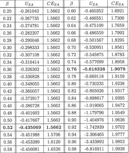
Thomas et Worrall (1988) étudient le problème de design de contrat entre un travailleur averse au risque et une firme neutre au risque lorsque qu’ils peuvent briser le contrat à tout moment. Dans ce chapitre, j’utilise la même approche pour expliquer les fusions. Jutilise des fonctions d’utilité de type CARA, ce qui permet de dériver explicitement le contrat optimal. Ensuite, j’ajoute quelques hypothèses pour évaluer les effets d’une fusion entre cIeux firmes ayant des revenus aléatoires. Pour ce faire, nous effectuons des simulations numériques. De part les résultats, une fusion est souhaitable seulement lorsque les agents ont un bas facteur d’escompte.

Mots- C lés Monitoring, Monopoleur multi-produit, Préférences multidimensionnelles, Biens indivisibles, Cycles, Rationalisabilité, Contraintes auto-excécutoires, Fusionnement, Contrats optimaux.

111

English summary

Chapter 1

The main purpose of the paper is ta introduce the decision ta monitor sales or nat in the multiproduct monopoly decision problem. Ta do sa, I intraduce the concept of a rnonitored contract as contract that consumers can buy only once. On the other hand, a non-monitored contract cottld be purchased in any quantity. Obviously, ta offer a monitored contract, the monapoly should 5e able to observe and ta control consumers’ choice. I find that the rnultiproduct monopoly vi1l aiways offer at least one non-rnonitored contract ta consurners.

Chapter 2

I study the composition of the Paretian allocation set in the context of a fuite number of agents and a finite number of indivisible goods. Each agent receives at rnast one good and no monetary compensation is possible (typically called the house allocation problem). I introduce the concept of a cycle which is a sequence af allocations where each allocation is linked to the follawing allocation in the sequence by the same switch of goods between a subset of agents. I characterize tlie profiles of agent preferences when the Paretian set lias cycles.

Chapter 3

Tliomas and Worrall (1988) study the problem af designing a contract between risk averse workers and risk-neutral firms when bath of them could break the contract at any time. In this paper, 1 use the same approaci ta study mergers. I model a CARA utility function ta derive explicitly the optimal contract and the value function for bath agents in the case where only twa states of nature are passible. I use this approach ta explain the reasan for a firm ta merge with anather one. Because the analytic solution is too difficult ta derive explicitly with more than twa states af nature, numerical simulations are used ta illustrate these cases. I find that mergers will occur anly when agents have a law discount rate.

Keywords : l\’Ionitoring, Multipraduct manopaly, Multidimensional Preferences, In divisible goads, Cycles, Ratianalisability, Seif-enforcing constraints, merger, Optimal Contracts.

iv

Table des matières

Résumé en francais j

English summary

Table des matières iv

Table des figures y

Liste des tableaux vi

Dédicace viii

Remerciements ix

Introduction 1

1 Monitoring Costs for a Multiproduct Monopoly 1.1 Introduction 1.2 Model 1.2.1 Multiproduct rnonopoly 1.2,2 Consumers 1.3 Resuits 1.4 Remarks on assumptions 1.5 Conclusion 1.6 References

2 Cycles and the House Allocation Problem 2.1 Introduction

2.2 Definitions and Notations

2.3 Properties of cycles and complete cycles 2.4 Cycles and Paretian sets

2.5 Conclusion 2.6 References

3 Self-enforcing contracts, value functions and CARA utility functions

with an application to mergers 49

3.1 Introduction 50 3.2 MocIel 52 4 25 26 27 28 29 30 36 41 47 47

V

3.3 CARA utiÏity functions 54

3.3.1 Conditions for a non-trivial solution 56

3.3.2 Pareto Frontier 64 3.4 Variance 79 3.5 Merger $2 3.5.1 Stand-alone case 83 3.5.2 Merger case 85 3.5.3 Results 8$ 3.6 Conclusion 94 3.7 References 95 Conclusion 97 Bibliographie 99

Table des figures

1.1 Non-Degeneration of the Set of Preferences 10

2.1 Allocation z and the cycle C (i,y) 43

2.2 Allocation z : first case 43

2.3 Allocation z : second case 44

2.4 Allocation z third case a 44

2.5 Allocation z third case b 44

3.1 first Constraint 59

3.2 Second constraint 60

3.3 Both Constraints 60

3.4 first-Best Contracts and Constra.ints 64

3.5 Unconstrained Pareto froritier 66

3.6 Stationary contract 68

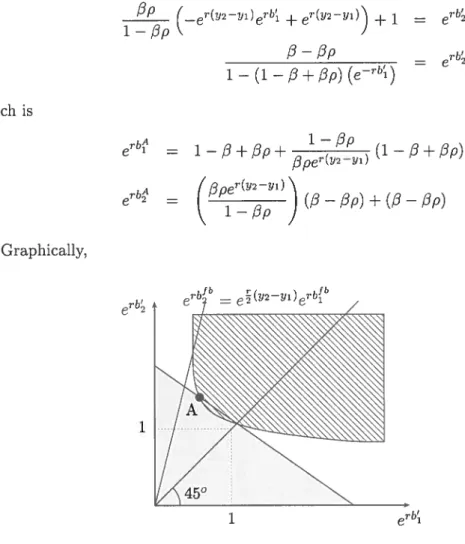
3.7 Pareto frontier with no self-enforcing first-best contracts 78 3.8 Pareto Frontier with self-enforcing first-best contracts 79

3.9 Certainty Equivalent 85

3.10 Negative Correlation and Merger 89

3.11 Positive Correlation and IVierger $9

3.12 Certainty Equivalent for tire stand-alone case and tire merger case with

p=—l 90

3.13 Certainty Equivalent for tire stand-alone case and the merger case with

p= —0.5 91

3.14 Certainty Equivalent for the stand-alone case and tire merger case with p = 0 93 3.15 Certainty Equivalent for the stand-alone case and the merger case with

vii

Liste des tableaux

I Utility of firrn 1 in the stand-alone case 84

II States of nature 85

III Coefficient of correlation and states of nature $6 IV Net gain of utility from the merger (positive value in bold) $7

Dédicace

À

Lucien et MarieÏle...

pour Ïa personne que je suzs,

A Véronique...

pour la personne que je veux être,

À

Daphnée et ses frères et soeurs...

pour la personne que je serai.

ix

Remerciements

En premier lieu, je tiens à remercier mes directeurs, les professeurs Walter Bossert et Lars Ehiers, ainsi que les professeurs Yves $prumont et Michel Poitevin pour leur disponibilité, leur professionnalisme et leur dévouement. Leurs nombreux commentaires m’ont permis d’acquérir une discipline certaine dans la rédaction d’articles scientifiques.

En second lieu, je ne peux passer sous silence l’impact de Yves Richelle sur mon chemine ment académique. Il fut un élément important du succès de mon doctorat. J’ai le privilège de l’avoir comme ami.

En troisième lieu, ma famille et mes amis ont eu un rôle non-négligeable dans la rédaction de ma thèse. Depuis presque 4 ans, ils ont dû supporter mes variations d’humeur au grès de la rédaction. Quelques fois, ce ne fut pas une mince affaire.

Pour terminer, je remercie le CIREQ, le SSHRC et le FCAR pour leur contribution fi nancière ainsi que le Bureau de la concurrence pour m’avoir permis de terminer ma thèse.

A distinctive Jeature of mzcroeconomzc theory is that it aims to rnodet economic acti vity as an interaction of individuat economic agents pursuing their przvate interests.

IVias-Coleil, Whinston and Green [8].

Les incitations économiques sont à la base des décisions des individus dans la vie de tous les jours. Que ce soit pour l’achat ou la vente de biens, l’offre de travail ou d’élection, les individus choisissent l’option qui, en fonction de la situation à laquelle ils font face, maximise leur bien-être. La modélisation microéconomique des décisions individuelles des agents constitue donc un outil privilégié pour l’analyse de questions aussi intéressantes que diversifiées comme le design de contrats d’assurance, les stratégies de mise en marché ou encore les problèmes d’allocation de biens indivisibles entre individus.

Dans le premier essai de ma thèse, j’étudie le comportement stratégique d’une firme ayant un pouvoir de monopole sur plusieurs marchés. Plus précisément, l’objectif est de mieux comprendre comment la firme décide d’effectuer du monitoring ou non. Je définis le monitoring comme la capacité pour la firme de suivre et de contrôler les achats de ses biens.

Pour vendre ses produits, la firme multiproduit peut avoir recours à la vente groupée (bundling) ou à la vente séparée. Par exemple, la plupart des chaînes de restauration rapide offre la possibilité d’acheter divers biens sous forme de trios. Lorsque les demandes ne sont pas unitaires1, la firme peut décider d’offrir des contrats qui ne peuvent être achetés plus d’une fois. Dans ce cas, nous dirons que le contrat est monitoré. Si la firme ne contrôle pas le nombre de fois que les consommateurs peuvent acheter un contrat donné, alors nous dirons que ce contrat est non-monitoré.

Jusqu’à maintenant, l’étude du monitoring se faisait au niveau des conséquences de ‘Nous disons qu’une demande est unitaire quand les consommateurs obtiennent un gain d’utilité seule

ment de la première unité de bien consommée. Une laveuse et une sécheuse sont des exemples de biens pour lesquels les consommateurs ont des demandes unitaires.

2

monitorer ou non. La quasi-majorité des articles sur la tarification non-linéaire2 utilisent implicitement (ou explicitement) l’hypothèse que la firme est capable de suivre et de restreindre les possibilités d’achat des consommateurs. La possibilité de ne pas monitorer fut étudiée exclusivement par Katz [5]. Cependant, aucun article ne modélise la prise de décision de monitorer ou non.

Dans cet essai, je présente un modèle qui incorpore la décision de monitorer ou non pour un monopoleur multiproduit. Une firme utilise le monitoring si elle offre au moins un contrat monitoré. Cependant, il est important de souligner que la décision de monitorer n’impose pas de monitorer tous les contrats. Il est toujours possible pour la firme d’utiliser des stratégies mixtes lors de la mise en marché des contrats. Un premier résultat est que, peu importe la fonction de coûts administratifs, la firme va toujours offrir au moins un contrat non-monitoré. Ce résultat est cohérent avec les observations. Il semble que l’ensemble des firmes offrent toujours la possibilité aux consommateurs d’acheter un type de contrat sans contrôle sur la quantité de fois qu’ils achètent ce dit-contrat.

Dans le second essai, le sujet d’étude est la rationalisation d’un ensemble de réalisations dans le cadre d’allocation de biens indivisibles (House Attocation Probtem). J’entends par rationalisation d’un ensemble A l’existence d’un profil de préférences individuelles qui a comme ensemble des optimums de Pareto l’ensemble A. L’allocation de biens indivisibles est un problème commun dans la vie de tous les jours. On peut penser à la répartition des chambres parmi des colocataires, les charges de cours entre professeurs ou aux espaces de bureaux entre collègues de travail. Ce type de problème fut introduit par Shapley et Scarf [12] et étudié par de nombreux auteurs dont Roth et Postlewaite [11], Svensson [13] et Elilers [3].

L’objectif de cet essai est d’introduire le concept de rationalisation dans un cadre d’allocation de biens indivisibles. Pour ce faire, j’introduis le concept de cycle qui consiste en une série d’allocations où chaque allocation est liée à la suivante par la même règle de transition. Un premier résultat découlant de la présence d’un cycle dans l’ensemble des optimums de Pareto est que tous les individus doivent avoir les mêmes préférences sur les biens qui se suivent dans le cycle. Deuxièmement, si le cycle est composé d’un nombre premier d’individus, alors tous ces individus doivent avoir les mêmes préférences sur les biens qui composent ce cycle. Troisièmement, je trouve que si l’ensemble des allocations parétiennes contient un nombre minimal de cycles composés des mêmes individus et des mêmes biens, alors tous ces individus doivent avoir les mêmes préférences sur ces biens. Comme quatrième résultat important, je trouve des conditions sur le nombre d’allocations que l’ensemble des optimums de Pareto doit contenir.

2Voir par exemple Goidman, Leland and Sibley [4], Mirman and Sihley [10], McAfee and McMillan [9] ou Armstrong [1].

Le troisième essai étudie les conséquences d’une fusion dans le cadre d’un modèle d’as surance avec contraintes auto-exécutoires. Nous disons qu’un contrat est auto-exécutoire si, pour tous les états de la nature et pour toutes les périodes, les deux agents (l’assureur et l’assuré) ont un gain à respecter le contrat. Sans contraintes auto-exécutoires, le manque d’engagement devient un problème. Lorsque les coûts de faire respecter le contrat sont élevés et que les coûts de changer de contrat est bas, un agent peut avoir intérêt à briser le contrat suite à la révélation de l’état de la nature alors qu’il était optimal ex-ante. Dans le but d’éliminer ce type de problème, j’utilise la même approche que celle introduite par Thomas et Worrall [14].

Dans la première partie de l’essai, je suppose que les individus ont des préférences qui peuvent être représentées par des fonctions de type CARA (Constant Absotute Risk Aver

sion). Cette modélisation se distancie de celle de Thomas et Worrall [14] et se rapproche de celle de Kocherlakota [6] en ce sens que les deux agents sont averses au risque. Avec cette hypothèse, je suis en mesure de solutionner explicitement le contrat optimal en supposant que les deux individus ont le même coefficient d’aversion au risque. Sans cette hypothèse, je ne peux expliciter la solution. Puisque nous trouvons le contrat optimal dans toutes les situations, je peux définir et tracer les frontières des optimums de Pareto selon les valeurs des paramètres. Les graphiques illustrent clairement que les frontières sont continues mais non pas dérivables en tout point.4

Dans un deuxième temps, je me suis intéressé aux effets d’une fusion entre deux firmes ayant des revenus aléatoires en présence de contrats auto-exécutoires. Pour ce faire,

j

‘ai modélisé deux firmes averses au risque qui ont un revenu aléatoire et un agent neutre au risque (le marché). Une des firmes peut décider de ne pas fusionner ou d’acheter l’autre firme au prix donné par l’équivalent certain. Dans le cas de la fusion (acquisition) ou de la situation ex-ante, les deux firmes ont la possibilité de signer des contrats d’assurance auto-exécutoires. Avec l’aide de simulations numériques, je trouve qu’une fusion peut être profitable lorsque le taux d’escompte est bas même lorsque les revenus des firmes sont corrélés.

4Kocherlakota [6] avançait faussement que les frontières des optimums de Pareto étaient continues en tout point. Ceci fut corrigé par Koeppl [7].

Chapitre 1

Monitoring Costs for a

Multiproduct Monopoly

1.1

Introduction

Firms combine different methods to seil their products. For example, many fast-food restaurants offer discount coupons on a specific meal while they allow consumers to buy any quantities of meals at regular prices. In construction material stores, srnall buyers face regular prices while big buyers have special discounts on their purchases. Defining monitoring as the control of consurners’ purchases, these examples suggest that firrns use monitoring in combination with usual non-rnonitored sales rnethods to maximize their profit.

The first context where such control on consumer purchasing is studied in the economic literature is the case of bundiing that offers consumers the possibility to buy a package in addition to the possibility of buying goods separately. The first complete model that deals with the ability of a monopoly to offer bundies vas proposed by Adams Yellen [1]. These authors study a market for two goods where consumers have unit demands for both products and they find that bundling can be efficiently used to increase firm profits even though consumers’ utility for each good are unrelated. Some extensions to the Adams & Yellen’s paper were made by introducing a joint distribution of consumer preferences over the two goods as in Schmalensee’s [9] model. Monitoring in such a context gives the monopoly the ability to restrain the set of possibilities available to consumers. For instance, with monitoring, a monopoly that wants to seli two goods can offer these goods separately as well as in a bundie, but can force consumers who want to buy both goods to purchase the bundie. The profitability of such possibilities to restrict the opportunities available to consumers are analyzed in IVIcAfee, IVicIViillan and Whinston [7]. These authors present sufficient conditions over the joint distribution on consurners preferences under which bundling gives more profits than selling goods separately when consumers are monitored. A second context where monitoring could be interesting to use is the case where firrns cari practice some form of nonlinear pricing (usually called second-degree price discrimi nation). Nonlinear pricing exists when a firm in a single market sets different unit prices for different amounts of goods purchased. Spence [10] presents a model in which a cen tral planner must maximize the aggregate consumer surplus without having the ability to identify the consumer’s type but with the ability to monitor consumers, by observing the quantities they buy. Goidman, Leland and Sibley [3] study explicitly the role of constraints on the price structure. They find that the price could be either upward or downward dis continuous in quantity with smooth and well-behaved demand and cost functions. $ince the 1980’s, many papers deal with the use of nonlinear pricing by a multiproduct mono poly. lVlirman and Sibley [8] assume that consumers differ by only one taste parameter while I\’IcAfee and McMillan [6] examine the case where multidimensional consumer pre ferences can be represented by a single variable. In this last case, the analysis becomes

6

identical to Mirman and Sihley’s. The first paper considering multidimensional preferences in a nonlinear pricing context is Armstrong [2]. Armstrong examines the decision problem of a monopoly over many goods facing consumers with multidirnensional preferences and flnds a method to resolve the mechanism design problem for some specific classes of cases. Except for the paper by Katz [5], which studies the case when purchases are not observable hy the firrn, ail papers on nonlinear pricing assume that the firrn is able to monitor purchases. In Katz’s [5] paper, the case of a firm with monopoly power on a single rnarket which is not able to observe consumer purchases is anaiyzed and a characterization of the optimal price schedule is obtained.

To my knowiedge, no paper examines the ability of a multiproduct monopoly to decide to monitor consumers purchases or not. The main purpose of the present paper is to analyze a model where the decision to monitor or not to monitor is an endogenous decision. To do so, I first define a contract as a vector specifying a quantity for each good and a price that will be paid by the consumer in exchange of the specified quantities. Then a contract will be said to he monitored whenever consumers can buy such a contract only once, while a non-monitored contract is a contract that consumers can buy without restrictions. In such a framework, the decision to monitor corresponds to the decision to offer a rnonitored contract. However, monitoring is lot an ail or nothing decision. Indeed, the monopoly can actually propose monitored contracts together with non-monitored ones. The main resuit is that the set of contracts offered by the monopoly wiil aiways contain a non-monitored contract. This accords with the exampies given above.

The paper is organized as follows. In Section 1.2, I introduce the model. The theorem of existence and sorne characterization of the optimal strategy of the monopoly are described in Section 1.3. Section 1.4 contains discussions on the basic assumptions and I conclude in Section 1.5.

1.2

Model

I consider a situation where a multiproduct monopoly faces N consumers. Let N be a natural number. The purpose of this section is to introduce the concept of monitored and non-monitored contracts as well as the assumptions relative to the behavior of the rnonopoly and of the consumers.

1.2.1

Multiproduct monopoly

A monopoly produces L goods and selis these goods tlirough contracts. I assume that the firm is risk neutral. The problem of the moiopoly is to determine the number of contracts as well as the composition of the contracts it wiÏl offer to the consumers. I define a contract as a vector that specifies a quantity for each good as well as a price that the

consumer who accepts the contract will pay in exchange for the quantities specified in the contract. Precisely, a typical contract k is given by (qi, ...,qi, ..., q,P) where q stands for the quantity of good t that will be sold if the contract is accepted and P is the price paid whenever the contract is accepted.

I also assume that the price elernent P is greater than or equal to E with c > O. As we shah see, this assumption is quite innocuous but xviii facilitate some of the arguments made below.

I begin by describing the kind of contracts that can be proposed by the monopoly.

Monitored and non-monitored contracts

In this paper, I say that a contract k is monitored if consumers cannot buy this contract more than once. In addition, I assume that consumers can buy only one monitored contract.

for non-monitored contracts, I assume that these contracts can be bought many tirnes and in combination with other contracts. To illustrate how monitored and non-monitored contracts work, consider the following example.

Suppose the monopoly offers txvo monitored contracts k and kb and two non-monitored contracts k and k. Following the definition of a non-rnonitored contract, the contracts given by uk3 or + uk for , cr = 1,2, ... can be bought by consumers. following the definition of monitored contracts, the contracts kC and kb are offered to consurners but not k + kb or ukb or + ukb since consumers can buy at most one monitored contracts and do so only once.

In addition to these contracts, it is possible for consumers to buy a combination on non-monitored contracts and one monitored contract. So the contracts given by k + k + k + + kb + kb + 5k and kb + + are offered to consumers.

To summarize, if the rnonopoly offers two monitored contracts kc and kb and two non-monitored contracts k and k, then the fohowing contracts are in effect offered to consurners for à, u = 1,2,3,

ka, _{kf’, k, k} uk, ka+uk k + k + uk, k + Sk + uk kb+k, kb+uk, kb+ka+Jk

Let K’’ and IQ’ be respectively the set of monitored contracts and the set of non-monitored contracts. With these sets, it is possibie to construct the contract set K(Km, I(’) which is the set of contracts which can be bought by consumers. Consi dering the preceding example, the set of monitored contracts K is given by {ka, kb}, the

8

set of non-monitored contracts by {k, k’} and the set of offered contracts by ka, kb k, k

Ska,uk,ka+uk S,u1,2,... K(Km K’m)

kb+kakb+Gkkb+ka+Jk

These definitions have three immediate implications that must be noted. first, whe neyer the set of non-rnonitored contracts is empty, the set of proposed contracts coincide with the set of monitored contracts, i.e., K = _K(I(

O).

This follows from the definition of a rnonitored contract. A second implication is that any contract kil _{e K(Km, Kfl) i}

either a monitored contract and belongs to K or an non-monitored contract and belongs to or a combination of non-monitored contracts and at most one monitored contract. Thirdly, since the ail elements of a contract are a real number, the sets of monitored and non-monitored contracts are countable. This implies immediately that the contract set is also countable. Furtherrnore, if K’T1 1nTrt

O,

then K(Km,K1m) =

O.

This means

that inaction is possible for the monopoly.

The next step in the description of the model is to present assumptions relative to the rnultiproduct monopoly cost structure.

Monopoly’s production and administration costs

Total costs for the monopoly consist of a production cost function which, as usual, gives the cost associated with the provision of a given quantity of goods to the consumers, and of an administration cost function which gives the cost to manage the set of proposed contracts.

The function V 1R — R+ gives the production cost which only depends on the

total quantity of goods provided to consumers. Let

_Q

(N, K, K7m) be the vector of total quantity of each good produced. I assume further that the marginal production cost is constant.1 So the production cost function becomes

V(Q(N,Km71(’1m)) = (c1 * Qt(N,Km,K))

where cj is the marginal cost of good I and Qi (N, J7n, IQm) is the total quantity of good I produced. I assume also that c1 > O for all t.

Note that I assume that the production costs do not depend directly on the number as well as the kind of contracts in the set of proposed contracts. Only the total quantity

of goods matters.

The function A represents the administration cost. I shah define A” as the cost function to administrate the non-rnonitored contracts while the cost function to manage the monitored contracts will be denoted by A. I assume that the cost of providing non-monitored contracts and the cost of providing monitored contracts are (directly) in dependent. I then assume that administration costs are additive in the non-monitored contract cost function A’ and the rnonitored contract cost function A

Regarding the non-rnonitored contract cost function, I assume that the cost to provide one more non-rnonitored contract is constant. This means that

A’ — flTfl

with aTlnl > O and where X denotes the number of elements of the set X.

For the cost to administrate monitored contracts, I assume that the number of consu mers buying a rnonitored contracts matters. This comes from the fact that, in order to make such contracts effective, the rnonopoly must follow each consumer to prevent multiple purchases of these monitored contracts, which imposes a cost to the monopoly.

Let Nm(N, 1rn, I7t) be the number of consumers who choose a monitored contract proposed in K(Km, _{Kfl) or a contract in i((Km,}Kfl) _{that is a linear combination of}

contracts, one of them being a monitored contract. This number is unknown by the firm since the firm does not know consumer types. Nevertheless, once the firm determines the sets of non-monitored and monitored contracts, consumers make their choice and their action generates the monitored contract cost function. I have mentioned above that the cost of providing a monitored contract does not relate directly on the set of non-monitored contracts. \Vith the hast assumption, the monitored contract cost function now depends indirectly on the set of non-monitored contracts since the latter affects the number of consumers buying a monitored contract.

Next, once again for simphicity, I assume that the monitored contract cost function is given by

A(NTT(N,Km7K’m),Km) = Kmam(Nm(N,Km,K7m))

Note that the assumption that the administrative cost is increasing in the number of consumers buying a monitored contract implies that am(.) is also increasing in N. I further assume that the unit administrative cost of a non-monitored contract, anm, strictly smaller than the unit administrative cost of a monitored contract am(.), _whatever

the number of consumers buying a monitored contract N.

Accordingly, the larger the number of consumers choosing a monitored contract, the harger are the costs associated with the management of monitored contracts and therefore

‘o

A

60

e

e

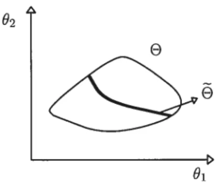
FIG. 1.1 — NomDegeneration of the Set of Preferences

I have Atm (Nl,Km) > Atm (N2,Km) whenever N’ > N2.

To surn up, a.ssumptions imply that the administrative cost function of the monopoly can be rrjtten as

A(Nm(N,Km,Im),Km,Km)= K ahtm + Km atm (Nrn(N,K,Khirn))

with ahitm _{> O.}

1.2.2 Consumers

The utility level attained byconsumeri whenever lie buys contract k’ = (qÇt... ,_q’,P”)

is given by u (6’,q, ...,q)

— Ph where O’

= (6f,... , 9) is a vector of preference parame

ters, i.e. preferences of consumer i with S > L — 1. I shah assume that u is continuous in

q1’ and in 6, increasing and strictly concave in q’ and satisfies

lim q)0 t=1,...,L VqO,jt, VOeO

qt—*oo

Note that individuals with the preference vector 6’ have the same utility function. The

set of ail preference vector, denoted by

e,

is a compact subset of R9. Preference vectors are i.i.d according to the continuous probabiiity distribution F(6). I also assume that f(O) is non-degenerative, i.e., the probability that O’ e

e

for ail

e

C

e

with Dirn[O] < Dim[] is zero. This assumption is commoniy used in the economic literature. For instance, if

e

lias only one dimension and the distribution is non-degenerative, the probabihty of getting a specific is equal to zero. Figure 1.1 represents a case where

e

is of dimension one whiie

e

is of dimension 2.

In this paper, I also assume that consumers could buy nothing if they wanted. In O’

this case, I say that the consumer buys the nuil contract k0 = (O, O, O,

...,

O). Then, the

problem of the consumer is to maximize his utility by choosing a contract in the set K0 which is the set of contracts offered by the firm K(Km, _{plus the nuil contract i.e.}

Ko(Km,K’m) = K(Km,K”m) U {ko}.

Let me denote by K (6i, 1cm, the set of contracts inthe set which maxirnizes the utility of consumers whose preference vector is O. I can immediately ask if there exist consumers whose K* (&i,1(fl,K7m) contains several contracts. To avoid this possibility,

I must add an assumption on utility function. The monotonicity in utility difference tvill guarantee that the set of optimal contracts is a singleton for almost ail types of consumers.

Definition 1.1 A utitity function (8f, q”) is -monotone if, foT alt q’, q2 suck that

q’ q2, s E {1, ..., S} such tit VO’ E

e,

u (O, q’) —u (Oi, q2) is strictty monotone in O.

The -monotonicity says that, for any pair of contracts k’, k2, if there is a such that k’ and k2 give the same utility, then an infinitesimal change in increases differently the utility of each contract. One can say that if a function

_f

is An-monotone, then

02f(O, q)

>

32f(&,

q)

8qt808

In fact, ,,-monotonicity is more than that. Take the function

f(&,

q) = &,(q, + q)2.

This function has positive cross-derivative if q and q are positive but it does not respect the Z\,,-monotonicity. Take the contracts q1 (1, 2) and q2 (2, 1) for example. For ah values of O, the difference in utility with those contracts will remain O. If a function is ,,_

monotone, then each marginal utility associated with a given good is affected differentially by a change in a specific preference parameter.

By assuming that the consumer utility functions are -monotone, then I obtain the foliowing result.

Lemma 1.1 The probabitity of finding a profite O E

e

such that Kt (oi, Ko) contains more than one contract is equat to O.

Proof. Take two contracts k’ and k2 betonging to K. Let be the set of alt preference uectors such that, for att E ,k’, k2 E K*

(,

Ko) and tet 0’ betong to

.

Fottowing the definition of Kt (O’,Ko), if k’,k2 E Kt (0’,Ko), then

(1’ 1 1 D’ — (j1 2 2\ j2

uJ i —ui _,q,,...,qL)

Fottowing the definition of the /-monotonicity, there is a s E {1, 2,

...,

S} such that u (0,q’) — u (0,q) is monotone in O.

Now, suppose there is an eÏement 02 betonging b such that 0 O. Because 02 E

e

and by L-monotonicity, there is another preference parameter t E {1, 2,

...,

S},t

s such

12

that 0 6 If not g2 cari not betong to . This means that any change in the parameter s teads to a change in some other parameter(s) to maintain the equatity

21 1 1 99 ₂ 9

u(0 ,ql,...,qL) —P =u(0,q,...,qL) —P

Then, the set

e

has a dimensionatity 1OWCT than

e.

By the non-degeneration of

e,

the pro babitity of having an agent with a preference vector betonging to is equat to O.

Since the contract set is countabte, I cari conctude that the pro babitity of having prefe rences such that theTe exist more than one optimat contTact is O. B

Note that this assumption of -monotonicity does not constrain too much as shown

by following example

Example 1.1 Take the case where the utitity function is represented by a square Toot function. Now, take two contracts k’, k2 such that q’ q2 and suppose that there is

o’

e

such that q’ and q2 betong to K*

(o’,

Ko). This means

0 (q)’2 + & (q)’12 =

&f

(q)l/2 + O (q)’12

Because q’ q2, there is at teast one t = 1,2, ...,L such that q q. Without toss of generatity, suppose that q > q Then,

& (q)’2 + O (q)’/2 — 0 (q)’2 + O (q2

increases if2 increases.

Because the contract set is countabte, the probabitity of having more than one optimal contract is O.

Note also that the Cobb-Douglas utility function u (O’, q”) = (q)Ol (q)O2 does not

respect the property of -rnonotonicity since when one quantity equals zero the utility levels are equal to zero irrespective of the value of O’. However the log transformation of the Cobb-Douglas utility will respect the A-rnonotonicity property.2

1.3

Resuits

The firrn’s problem can be described as choosing the number of rnonitored and non monitored contracts and the composition of each of them. I shah denote by n (N) the maximal profit the monopoly can obtain when it faces N consumers. By assuming that

21f I define the weak -rnonotonicity with adding that q; and q must be composed of positive elements,

the firm is risk-neutral, I cari write the profit function in the following way

ir (N)

= K”,Km E[R (N, Ktm, Ktm)

— C (N, Ktm, K7m)]

where R

_(.)

and C

_(.)

are respectively total revenues and total costs for the firm when

the chosen rnonitored and non-monitored contract sets are Krn and the number of consumers N.

I suppose that the firm is unable to observe consumer preference profiles and consurners are not allowed to resell the quantity bought from the firm. Let the term Pr (kh,_{Ktm, Kflm)} be the probability that a consumer buys the contract kIl, i.e. Pr (k”, jrn, Kam) =

Pr (i _E

e

_{k” E K*} (&i _{Ktm Knm)) Then, expected revenues cari be written as follows} E[R (N, Ktm, Ktm)] = N * (P” * Pr

(e’,

Ktm, Im)). kh EK

In the previous subsection 1.2.1, I define the cost function like the sum of the production costs and the administration costs, i.e.,

C(N, Ktm, K’’) = V (Q(N, Ktm, KTttm)) + A (N”(N, Ktm, K”), Ktm, K’tm)

By assurning that the production cost is linear in quantities, the production cost func tion is given by V

_(Q)

=

Z[Z1

(ct * Q1(N, Ktm, K’”’)). With the assumption of risk neu

trality by the firm, the expected value of the prodttction cost, E[V

_(Q)],

is given by

E[V

_(Q)]

= (c * E[Qt(N, Ktm, Ktm)])

E[Qt(N,Ktm, K”tm)] denotes the expected total quantity of good t produced by the firm and equals

N (qÇ*Pr(kh1,Ktm,Knm)) khEK(I(m,Knm)

In other words, the expected total quantity of good t is given by the sum (over the contracts belonging to the contract set K) of the quantity of good t specified in a contract tirnes the expected number of consumers buying this contract. It follows that E[V

_(Q)]

can be written as

E[V

_(Q)]

= N * (ci * q’ *Pr

(,

Ktm, Im))

t1

mon-14

tored contract cost function and the non-monitored contract cost function. The expected administrative cost function will therefore be given by

E[A (Nm(N, Im, K), Ktm,

_Km)1

IKI

aTttm + imi E[am (Ntm(N, Im, Inh1))1 Let a (N, Ktm, Km) be the expected value of atm (Nm(N, IQ’, Km)). With this no tation, the expected administration cost function becomes

E[G(N,Ktm,KT1m)] N * (ctqPr (kh,Im,Im))

1=1 khEK(Km,Knm)

+

K7I

atm _{+ Ktmi}a(N,Ktm, K’2T’) To sum up, the maximal profit the rnonopoly, rr(N), can 5e written as

(N) = N * pr

(,

i, im) (ph — (c1)) khK(Km,Krn) t=1 (1.1) — a1m — iKtmia (N, Ktm, K’)

Expressed in this way, there could 5e situations where -ir(N) does not exist since the maximization problem lias no solution. Indeed, whenever the contract set K contains a non-monitored contract, K lias an infinite number of elements so that the function to be rnaxirnized involves a sum over an infinite number of elements and this sum will not necessarily give a real number. I must therefore address this problem imrnediately. We have already seen that each contract can be expressed as a combination of non-monitored contracts and no more than one rnonitored contract. I can then rewrite (1.1) in terrns of non-monitored and monitored contracts instead of the whole set of contracts. However there are stili rnany possibilities whereby non-rnonitored contracts and monitored contracts can 5e cornbined to obtain the saine kh belonging to K(Km, Km). The first possibility is when there are suci that, for a given k9 belonging to Ktm U {k0}, kh can be written as

kIl _{= k9+ /3k} =

kKm

The second possibility is when kIl can be expressed as two different combinations of rnonitored and non-monitored contracts

kIl _{= k9+ j3k =}

_IJ+

with k, k belonging to Ktm

u

{ko}.

If no other structure is added, I could have a problem with double counting. Let me first define the lexicographic dominance of a vector. I say that a vector

_fi’

is lexicographically dominated by

_fi2

if

fi <fi?

or

_fi=fi?

and _/3<i3?

or

_fi

=

fi?

fi

= i? and

fi <fi

Let K = K7 U {ko} be the set of rnonitored contracts and the nuli contract. I define

W (kb, Ktm, for any kil belonging to K(Km, as the set of ah pairs of k’ be longing to K and

_fi

N1’ such that kil = k + ZkigKm Let w (kil, Ktm, Knitm)

be the pair (k9,

_fi)

belonging to W (kil, _{Ktm, Knm) such that}

_fi

_{is lexicographically domi}

nated by for ail other pairs (kf,) in W (kh,Km,Knm). (kil, Km, Knm) is unique because the lexicographic ordering is complete and transitive and if

_fi

= , then k = kf.

Let W (Ktm, K”tm) {w (k’t, Ktm, K”) kil E K(Ktm, K’m’)} and let

₍₎

=

{

C R

I

I17]}.

With ah the definitions introduced, I can write the profit maximization problem like a double maximization where the first one is made on the number of non-monitored and monitored contracts and the second on the composition of those contracts. Formaily,

n (N) = max max

77m ,Tlnm K’‘P(T1m),K’m‘P(’inm)

N I [(ko,

_fi)

E

W

(KT, Knm)j Pr (kil,

k!EK /3gNflm / / . .. (1.2) f l]nm L f llnm * (P9+fiiP—ci* {q+fijq1 1=1

_\

j=1 — i”m — K”’ a (N, K771, K71tm)

where I

[,

_fi)

E

W

(Ktm, 1(nimn)] is an indicator function which takes the value 1 if the condition is respected and O otherwise.

I have once again a summation over an infinite number of elements, but many of them are irreievant for the problem. Indeed, since the marginal utihity goes to zero when the quantity goes to infinity, for any ‘ _{beionging to O the utihity converges to a level} (Oi)

when quantities go to infinity. The utihity function being continuous in O, the function (6) is also continuous in 6’. Accordingly, there is a 0’

e e

maxirnizing (0’). Let

16

Because the utility function is quasilinear in price, the maximum revenue the firrn could earn is given by NMAX. for a number 77 of contracts offered, the minimal administration cost3 is given by 77a7m. _{This implies that the maximum number of non-monitored and}

monitored contracts is equal to NX since, otherwise, the firm’s profit will be negative with probability 1. Let B {t3 E

N”I

Z7’î

< Nï’.r4x

}•

It now follows that Problem

(1.2) can be equivalently written as follows n (N) = max max 71m,T1rm KmEP(71m),KmEIi(71um) N * I [(9,

)

W

(Ktm, K7im)] Pr (kft, Ktm, Ktm) kEK /3eB (1.3) ?7rini L TInm * P+t3jP—ct* _q+/3jq j=1 1=1 j=1 — K’ a’ — K77 a’ (N, Ktm, K’m)

The maximization problem is now well defined. I now show that this problem lias a solution.

Proposition 1.1 For any finite number of consumers, there is a sotution to the profit rnaxirnization probtem (1.3).

Proof. I proceed in four steps. The first step is finding the contract k* (9’) which is the contract (q* (yi) , p* (oi))

such that

q* (gi)

= argrnax u (9,q) — ciqt (1.4)

p* ₍₉₎

= u (9 q* (9’)) (1.5)

By the concavity of the utitity function and by the assumption that the marginal utility goes to O when the quantity goes to inftnity, there is a solution to (1.4) amI (1.5). Atso, with the assumption of strict concavity, k* (O’) is unique4. I define n* (O’) the profit given by the contract k* (Oi), i.e.,

n* (gi) = p* (gi)

— ctq

(ei)

Let q[IA’ be the maximum quantity of goods t a consumer of type O’ E

e

obtained in

3Remember that the cost to offer a rnonitored contract exceeds the cost to offer a non-monitored contract.

k*

_(),

_i.e.

qfVIAX

_ max q

(0i)

By the continuity of the utitity function in & and the compactness of

e,

q(VIAX is upper bounded. I can proceed by the sanie approach with pMAX and MAX

pMAX

= max p* (0i)

EO

= max ir (&i)

E e

I then define the set L.

= {(q, P) qt

e [o,

q(X] VI = 1,2,

...,

L, and P

e [o,

pMAx]}

Note that L is a compact set by construction.

As atready discussed above, I show in the second step that the flrm couÏd onty offer a finite number of monitored and non-monitored contracts. If the number of consumers is N, then the maximum profit the firm coutd obtain without counting the administration cost A (Nm(N,K, frflm), K, K’’) is I ij the maximum number ofmonitored

and non-monitored contracts the fin coutd offen with the possibitity to make a profit. With

the assumption that anm < am (T _(N,1cm, I(nm)), _{the maximum number of monitored}

and non-monitored contracts is given by

NM — îa?m >

o

—

(

+ 1) a <O

Because N7rMAX is upper bounded, that means the monopoty witt neyer offen an infinite number of non-monitored or monitored contnacts (i < oc).

The third step consists of proving that

N * i [(k9,

)

e

W

(Krn,K71m)] p (kh Im,Kj k9EK{ f3EB Inrn L ‘hrn * ₊ — cj * (q + 1.6 t;

_\

j=i —

IK’m

&m — K a (N, Ktm, KT’)

is continnous in q9 and pg for alt k belonging to Ktm and continuous in q and P3 for alt k betonging to K’’m.

‘s

The term I7Lm a is obviousty continuons since it is a constant. The expected mo nitored contract cost function j (N, K”, K”) is function of the number of consumers buying a monitored contract. Because I take the expectation and the distribution function of O’ is non-degenerative, then a (N, Km, K””’) is continuons 3 qZ _{and pz}

I now examine the terms in the summation. To do this tet me begin by defining t as

fJxiim J9 Tlnm+TIm

e vec OT _{tJj=1’1 t g=m+1}

Then and be the contract sets with ii,,, monitored contracts and 7],,, non monitored contracts. I define and Kmt the monitored ami non-monitored contract sets such that = + 5’ fo att‘ betonging to

J

and = + c5 for alt

?

betonging

to K”.

To prove the continuity of the terms in the summation in (1.6), I must discuss two cases.

The ftrst case is when, for att betonging to

J,

for alt

_/3

betonging to

Ê

and for any sequence {St} that converges to the zero vector whenever t tends to infinity, the indicator function i

[(,)

e

w

(t,K71mt)] = i

[(,)

e

w

(,K7im)] for att t. In this

case, the sum of the indicator function times the pro babitity becomes a sum of pro babitities. By definition,

if

the indicator function is equat to 1 for a given pair (k9,

_/3),

then there is no other pair (kf, j3f) with k1 betonging to

k

and

_/3

betonging to B such that k + L’ /3k3 = k1 + /3tki and such that /31 is lexicographicatty dominated by /3.

Then, I have to anatyze the effect of changes in q9, p, q and P on the probability

P (k” 1m Inrn) evaluated at k9 = ]‘, k = and K = j(fl?fl =

Let

7”

]‘ + /3i. By definition,

if!’

ê K

(&J,

Knim), then:

u(O,,...,)_P”rnax

k K0

By Lemma 1.1, the probabitity that an agent has a preference profite such that there are two contracts betonging to ir”

(o’,

Im, K”m)is

o.

Then,

Pr (kh, K”’, K”’”) =

Pr

(

u (O,,

_...,‘f)

— > maxz0 [u (O,,

Z) —z]

)

Because n (O,’) is continuons in O ami in j’ and because the distribution fnnction of the O ‘s is non-degenerative, I can use the Slutsky Theorem5 to prove that the probabitity is continuons in j9,9 _{for alt}

]?

_{betonging to K” ami in} ji,3 _{for alt betonging to}

The second case is when there is a pair

(,

/3)

with betonging to

J

ami

_/3

belon ging to

Ê

and a sequence of snch that, for att t >

i,

I [(kv,

_/3)

ê

W

K”m)]

_#

I e

W

(J,Knm)]

To begin with, suppose that, foT the pair (9,/3), I

[(r,i3) e

W

(J, J)]

= 1 an

i

[(g,

)

e

W

(i,

Knrnt)] = O foT ait t>

E.

ij I

[(r’,

/3)

e

W

(i,

)]

= 1, then

this means that, for alt pairs

(,

_{t3f) with}

]

betonging to

Ï?

and 13f betonging to

Ê

such that g + = +

_/3

is texicographicatty dominated by 13f• If I [(,t3) e W = fo t> t, this mearis that there exists a sequence

of pair

_{(,

/3Z)}t>î with betonging to it and /3Z betonging to

Ê

such that ]‘ +

Zi

/3] = +

_ZL

/3 and 3z is texicographicatty dominated by

_/3.

Note however that Y)nm ‘mm = j=1 7]alm ‘1,im 11m + /3zkJ = + j=1 j=1

Accordingty, I find that

7i’

+ /3! is equat to Z +

ZÏ

with /3z texi cographicatty dominated by t3. This teads a contradiction which impties that there does not exist a pair (9,/3) for which, for alt t >

E,

I e

W

()]

= 1 and

I[(/3)

eW(J)]—o

Now, suppose that, for the pair (°,t3) andforattt>

E,

I

t(9)

e

W

_t,KT’)] =

O andl

[(/3)

e

W

(Jt,Kflmt)] = 1. This means that there is apair (],/3f) with!

betonging to

7

and 13f betonging to

Ê

such that ‘+

_Z

/3 = _{+ zji;} and /3f texicographicatty dominated by 3. Without tost of generatity, suppose there is onty one such pair. If I

e

w = 1 for alt t>

E,

this means +

is not equat to +

/3fl.

Then, the probabitity that a consumer has preferences O such that either

(

+ or

(7

+ betongs to I(.

(&,i,7?)

is given by pr

(

E

eI+t3

E K (i)) +Pr e

ej[

+/3 E K* T/nrjj -Pr (oi

e

e

(+t3)

and

(+/3)

betong to i*

20

By Lemma 1.1, if + /3] is not equats to +

_Z

t3Çk, then the probabitity that a consumer has a preference profite such that +

7L

/33k and +

betongs to K is zero. But by taking the timit of the preceding sum of probabitities, I obtain

7

T/n ni

1im Pr

(&

e

+

e

K* (O,I,J)

i=1 ‘in in +Pr & e

e

K* (ijIçnm) i=1 iii ‘in in = Pr

e

eI°

+

e

K (0i))

t

+Pr (9

e

eIi

+

e

K* (6ijj) i=1 ‘mm ‘mm eK*(OiKnim)) ‘mm Pr O

_e

+ K (6ij) i= because

i

+ = k +

Then, by introducing the indicator function, I avoid double counting. I therefore have ‘irnt I

[(,)

e

W

Pr O

e

K* TInm +1

[({ )

e

W

()]

Pr

e

+

e

K* (Oj,t, Kmnit)) I

_[(r,

)

e

W

(r)]

Pr

(0

e

+

e

K (gi

,

Knm)) +1

[(,)

e

W()]

Pr

e

e

K* (OiKnm))

where i

[(, )

e

W

(it, Knmt)] and I

[(n,

i3)

e

W

_(i’

K7mt)] are equat to one white i

[(p,

t3)

W

(J,

Knm)] is equat to zeo and i

[(r,

/3)

e

W (],

Jn)] j equat to one.

Then, (1.6) is continuous in q9 and p foT alt k’ betonging to Ktm and in q1 and P

for alt k betonging to K’.

For’ tire fourtir step, let (77nm 77m) be tire maximum profit obtained when tire optimal contract must be composed of non-monitored COntTaCtS and 77m monitored contracts.

= max 7)nm N* _ZI[(k9,/3)

e

W(Kfh,KnTn)]Pr j=1

/

L

/

1=;

\

J=i

—

IKm

a’tm

—

iKm a (N, Ktm, K’m)

In tire previous step, I proue tiraI tire function (1.6) is continuons in qZ and Z

for alt kZ belonging to Km or to K. Moreover, non-monitored and monitored contracts must betong to z. Tiren, I use tire theorem of tire maximum to proue tirat (N, 77nm, 77m) exists.

Since 77 Z5 finite, tiren tire number of combinations of (77nm, 77m) witir 77nm +77tm <77 atso finite. Consequently, tirere is a maximal etement in tire set

22

I can now examine if the maximal profit ir(N) is strictly positive for any N. This could not necessarily be the case since I have assumed above that the monitoring cost function is increasing in N. It could for instance happen that the profit is strictly positive when there are 10 consumers but equal to zero with 11 consumers. However, as shown by the following resuit, I can state under certain conditions that profits vlll stay strictly positive when the number of consumers exceeds a critical level.

Proposition 1.2 Suppose that t E {1, 2,...,L} such that, foT alt

qh _with q1

= 0,

/

8u(Oi,qul)

_N

Pr(Oee

I

_h

>ctl

>0

)

There is a

N

such that VN > N, the profit is strictty positive.

Proof. Suppose that K =

0

aiid K” has onty one etement which maximizes

Pr(kut,ø,Knm) * (Pu1_(ct*q))

kIEK(ø,Km) 1=1

By assumption, I know that this ter’m is positive. Then, I can set

N

such that

N

* Pr (k1t,

O,

Knm) * (Ph —

(

* q)) — a”tm <

khEK(O,Krm) 1=1

(N+

1) * Pr (kht,o,Knm) * (Ph — (ci

*))

—a” >

o

k)EK(O,Km) 1=1

The condition for a strictly positive maximal profit is not a strong one. It says that if there is a positive probability to finding a consumer with a marginal utility over at least one good that is higher than the marginal cost to produce this good, then the firm makes profit when the number of consumers is high enough. The intuition for the proof is simple. When the number of consumers increases, the administrative cost to provide one non-monitored contract, which is constant with respect to N, becomes negligible. It will then become possible to make strictly positive profits whenever the number of consumers becomes sufficiently large.

Let me now study if the maximal profit increases when the number of consumers increases. The following result shows that this will depend on the form of the monitored contract cost function.

Proposition 1.3 If a (N, Ktm, Ktm) is concave in N, then the profit function is non decreasing in N. If there exists an for which the profit is positive, then the pTofitfunction is increasing for ail N N.

Froof. Let Km(N) and K?m(N) be the optimat monitored and non-rnonitored contract set when the number of consumers is N and tet K — K (Km(N),KhlTn(N)). By definition,

n(N+1) > (N+1) Pr(kh,(N),(N)) (Ph_(ci*q))

t1

—

IKm

a”tm —

ImIa

(N + 1, (N), (N))

where the right hand side is the profit when the number of consurners is N + 1 and the contract sets are Km(N) and Kntm(N).

n(N+1) (N+1)

[

Pr(kh,(N),(N)) (Ph_(ct*q1))] khEk tzrl Km a (N + 1,(N), (N)) —I(”ma”m—(N+1) N+1 By the concavity ofa (N,Ï(N),ï(N)) in N, then

a (N, (N), (N)) a (N + 1,(N), (N)) and therefore n(N+ 1) (N+ 1)

[

Pr (k”,(N),(N)) - (ct IhEk 1=1 a (N,ï(N),(N)) — i”” a”” — (N + 1) N n(N+ 1) > N

[

Pr (kh1,(N),m(N)) (Ph - (ct * khEK 11 a (N,i(N),Y(N)) — i”ma”tm — N

with a strict inequality

if

n(N) > O. Note that the .right hand side of this inequatity is simpÏy n(N) so that the resutts foltow. •

24

Without any assumptions on tire concavity of tire monitored contract cost function, it is impossible to obtain any conclusions about tire evolution of tire maximal profit ir(N)

with respect to tire number of consumers. It could irappen that the increase in the cost of monitoring contracts is more important than tire increase in tire revenue minus tire production cost. In this case, the profit will decrease.

Tire second interesting question regards the composition of tire optimal contract set. The first resuit found is that the monopolist will aiways offer at least one non-monitored contract. Tire following proposition demonstrates this resuit.

Proposition 1.4 Suppose K’ and K” are the optirnat monitored and non-monitored contract set. Then, there is at teast one non-monitored contract, i.e. K’”1

0.

Froof. Suppose that Km

_0.

By definition, K (Km,

o)

im. In this case the profit function is

N [Pr (kIL, Ktm, Knm) (ph —

(ct)) — a (N,,

o)]

khE ti

First, I know that the number of monitored contracts iffinite. If not, the fixed cost witt be infinite. consequentty, foT each monitored contract kh betonging to Km,

pr (kh,Im,Im) (P11

—

(ciqil))

— a (N,,O) >0 (1.7)

Ifthere is a contract in winch tins condition is not respected, I coutd drop tins contract out without decreasing the profit.

I define Ktm as the monitored contract maximizing (ph

—

zf

(ci

* _{q)). Let}

=

{}

andi =

{}.

The profit with

k

andi 9Vfl by

N i [t

e

W

(J,J?)]

Pr (k1,T,KtLm) kEI[ /3EB

t

TJnm L

f

P9+3jPi—Zct*

f

q’+/3q ji 1=1

_\

j=1 — a”tm —

J

a (N,

7,

K””)

By assumption, a’

_(.)

> a’’”. Hence, the administration cost of offering

i

and Km is tower tian tire cost of offering K’” and

O

respectivety as tire monitored and non

monitored contract sets. Tien, if tire first term witi tire contract sets J and

is not

smatter tian

witi Ktm

and 0, the

point is proven.

under the contract set K(Km,I(’”) : they can continue to buy the same contract, they can

stop buying OT the can change their choice fora new contract. By construction, K(Km,

0) c

K(i,7). Consumers who buy a contract undeT K(Km,

0)

will neyer choose not to

buy a contract when they face the contract set K(J?,

I)

because they decide to buy a

contract betonging to i

(o,Im,0)

and this contract is stiti avaitabte in K(,Knm). Then, consumers must choose between a contract betonging to i

(o,

im,

o)

OT ano ther contract. It is sure with probabitity equat to 1 that consumers witt not switch to another

contTact kh Km\

{}.

If they do, this means

(o,

I771,

o)

contains two contracts but the probabitity that i

(o,

Im,

o)

has two contracts is 0.6

Consumers reatty onty have two possibilities keep buying the contract they buy with the contract set K(Km,

O)

or buy a contract k which is a combination of the non-monitoTed contract and of at most one monitored contract.

=kh+ kheK,e{1,2,...} But

P

— (c

* >

— (c

*

)

which means that the first term of (1.7) is

greater with than with K. •

This resuit is very interesting. It says that every firm will offer at least one non monitored contract, which is what happens in the real econorny. Many stores offer some special discounts to big buyers and offer to others the possibility of buying without being monitored. The stores open an account for big buyers and offer a discount depending of the total purchases.

Which form of administration cost function is more likely to occur? The intuition says that concavity for the monitored contract cost function is a realistic assumption. The biggest cost of implementing monitoring structure is more a form of fixed cost. Sorne ob servations strengthen this intuition. Convenience stores almost aiways offer non-monitored contracts and superrnarkets offer discounts on a specific quantity of goods. Also, if there is an important flxed cost to implernent monitoring, only big surface selling stores will use monitored contracts. On the other hand, one can argue that it becomes more complicated to keep track of consumers as their number increases. Nevertheless, sorne technological implements can contribute to diminishing the monitored contract costs.

1.4

Remarks on assumptions

To develop the model, I use strong assumptions on the utility function, the production cost function and the monitoring cost function. I impose those assumptions to sirnplify

26

the presentation of proofs. IVlany of these assumptions could be relaxed to more general functions, however.

Regarding the utility function and the production cost function, I need assumptions which would guarantee the existence of a solution to the profit maximization problem. To have a solution, it must be the case that, there is a 4 snch that, for ail q 4, for ail

Q

q and for ail 9 E

e,

dv(Ql,...,QL) >

du(9i,q,...,q)

Vl=1,2,...,L

dQ1 dq1

In other words, the marginai utihty at 4 must be iower than the marginal cost to provide at least 4. For consumers, the assnmption of strict concavity in q is not necessary. The concavity is enough to have existence.

The assumptions about the monitoring cost function are more problematic to discuss. In fact, it is very difficuit to specify the form of this fuuction. It makes sense to have a monitoring cost function iucreasing in the number of base contracts but the linearity doesn’t look too realistic. But I do not need the linearity to prove its existence. I simply need the assumption specifying an increase of the monitoring cost when the number of base contracts increases.

A (Nm(N, Ktm, Krn), Ktm, K) > A (Nm(N,

_{), ,}

)

if

(Tjnm,7]rn)

(5,ij)

(77nm,7]m) (7nm,’]m)

where is the number of non-monitored contracts and iy is the uumber of monitored contracts. Without this assumption, I am not able to upper-bound the number of base contracts. In this case the uumber of contracts could be infinite and it is impossible to guarantee a solution to the profit maximization problem.

1.5

Conclusion

In this paper, I try to model the firm’s decision when it involves monitoring. I find some sufficient conditions to get an existence proposition. It appears that the main assumptions to gnarantee a solution are more about consumer preferences and the production function than about the monitoring cost function. I also find some results on the characterization of the optimal coutract set under specific assumptious.

Another issue involves the definitiou of monitoring. I define monitoring as the capacity to constraiu consumers to buy no more than one contract, when in fact, other definitions could also be used. For example, I could assume that a monitored contract could be bought

with or without another monitored contract. But using alternative definitions complicates the presentation of the resuits without providing additional insights on the problem of monitoring.

In my opinion, future work on monitoring should study the uniqueness of the monopoly solution problem. Uniqueness is not guaranteed under the assumptions introduced in this paper and it seems that stronger assumptions on the utility function would have to be made in order to obtain it. Another way to extend the present study of monitoring is by developing the characterization of the optimal contract set. Also, the approach proposed in this paper could be taken in the context of a regulated monopoly context in order to examine whether the use of rnonitored contracts could increase welfare.

Finally, introducing monitoring in a duopoly, oligopoly or perfectly competitive fra mework seems to be the natural next step. But it seems to me that this step will be very difficuit to take. The multidirnensional preference profiles and good vectors complicate the analysis of the stability of any optimal strategies. Furthermore, firrns will not compete only on quantities and on price, but also on the number of contracts and on their nature.

1.6

References

[1] W. j. _{Adams and J. L. Yellen. Commodity bundiing and the burden of rnonopoly.}

Quaterty Journal of Economics 90, pages 475—498, 1976.

[2] M. Armstrong. IVlultiproduct nonlinear pricing. Econometrica 64, pages 51—75, 1996. [3] M. B. Goidman, H. E. Leland, and D. S. Sibley. Optimal nonuniform pricing. Review

of Economic Studies 50, pages 305—319, 1984.

[4] J. Jacod and P. Protter. Probabitity Essentiats. Springer, 2002.

[5] M. IKatz. Nonuniforrn pricing with unobservable numbers of purchases. Review of Economic Studies 51, pages 461—470, 1984.

[6] R.P. McAfee and J. /IcMi11an. lVlultidimensional incentive compatibility and mecha nism design. Journal of Economic Theory 46, pages 335—354, 1988.

[7] R.P. McAfee, J. McMillan, and M.D. Whinston. Multiproduct rnonopoly, cornmodity bundiing and correlation of values. Quarterty Journal of Economics 103, pages 371— 383, 1989.

[8] L.j. Mirman and D. Sibley. Optimal nonlinear pricing for multiproduct monopolies. Bell Journal of Econornics 11, pages 659—670, 1980.

[9] R. Schmalensee. Gaussian demand and commodity bundling. Journal of Bussiness

57, pages 521—529, 1984.

[10] A.IVI. Spence. Nonlinear pricing and welfare. Journal of Public Economics 8, pages 1—18, 1977.

Chapitre 2

Cycles and the House Allocation

Problem

2.1

Introduction

The house allocation problem consists of the assignrnent of indivisible goods to a set of agents who can receive only one object in the final allocation. Such problems are very common : allocation of rooms between roommates, lectures between professors, offices between colleagues, etc.

This class of problems xvas introduced by Shapley and Scarf [8]. In their model, agents own ail goods collectively. Whule Shapley and $carf prove the existence of a competitive equilibrium, Roth and Postlewaite [Z] show that this competitive equilibrium is unique when preferences are strict over the set of goods. Roth [6] proves that this unique solu tion can be implernented by a strategy-proof allocation rnechanisrn. Furthermore, there is a unique strategy-proof, individually rational and Pareto optimal allocation mechanism leading to the unique core allocation (Ma [5]). Abdulkadirolu and $t5nrnez [1] show the equivalence between the competitive allocation from random endowments and the random serial dictatorship while Svensson [9] proves that all mechanisms that are strategy-proof, nonbossy and neutral must be serially dictatorial. Abdulkadiroglu and Sônmez [2] mo del the case where there exists at the sarne time tenants and new corners on the same rnarket. They introduce the top trading mechanism in this set-up and show that it is Pa reto efficient, individually rational and strategy-proof. Ehlers [4] introduces the possibility of having weak preferences over the set of goods and shows some restrictions on agent preferences with which efficiency and coalitional strategy-proofness are compatible.’

The purpose of this paper is to look at rationalizability in the context of the house allocation problem. In other word, I am interested in answering the following question is it possible to say if, for a given set of allocations, there is a preference profile which supports this set as a Paretian allocation set? In existing papers on the house allocation problem, only the paper by Ben-Shoham, Serrano and Volij [3] mentions explicitly the composition of the Paretian allocation set. They show that for any two allocations in the Paretian set, there exists a sequence of allocations belonging to the Paretian set such that they are pairwise connected, i.e. there are only two agents switching their goods and ail others stay with the same good. This means that a set with two allocations that are not pairwise connected cannot be rationalized.

To go further on rationalizability, I need to introduce the concept of a cycle. A cycle is a subset of allocations in which a subset of agents switch their goods according to a specific scheme. The presence of cycles in a given set of allocations which is presumingly a Paretian set gives us information on the potential preference profiles which would support this set as a Paretian allocation set. With the concept of a cycle, I derive sorne conditions regarding the number of allocations that have to belong to an allocation set in order for it