Cooperative-cum-Constrained Maximum Likelihood Algorithm for UWB-based Localization in Wireless BANs

HAL Id: hal-01175913

https://hal.inria.fr/hal-01175913

Submitted on 13 Jul 2015

HAL is a multi-disciplinary open access

archive for the deposit and dissemination of

sci-entific research documents, whether they are

pub-lished or not. The documents may come from

teaching and research institutions in France or

abroad, or from public or private research centers.

L’archive ouverte pluridisciplinaire HAL, est

destinée au dépôt et à la diffusion de documents

scientifiques de niveau recherche, publiés ou non,

émanant des établissements d’enseignement et de

recherche français ou étrangers, des laboratoires

publics ou privés.

Cooperative-cum-Constrained Maximum Likelihood

Algorithm for UWB-based Localization in Wireless

BANs

Gia-Minh Hoang, Matthieu Gautier, Antoine Courtay

To cite this version:

Gia-Minh Hoang, Matthieu Gautier, Antoine Courtay. Cooperative-cum-Constrained Maximum

Like-lihood Algorithm for UWB-based Localization in Wireless BANs. IEEE International Conference on

Communications (ICC15), Jun 2015, London, United Kingdom. �hal-01175913�

Cooperative-cum-Constrained Maximum Likelihood

Algorithm for UWB-based Localization

in Wireless BANs

Gia-Minh HOANG, Matthieu GAUTIER, and Antoine COURTAY

gia-minh.hoang@etudiant.univ-rennes1.fr, {matthieu.gautier, antoine.courtay}@irisa.com

Abstract—Wireless Body Area Network (BAN) is a mainstream technology for numerous application fields (medicine, security, sport science. . . ) and precise determination of wireless sensors’ positions responses to the great needs in many applications. In addition, Ultra Wide Band (UWB) radio is an attractive technology to achieve the centimeter-level distance measurements. However, the aggregation of the distance information remains a challenge and this paper presents a cutting-edge method for performing the accurate localization in wireless BAN. To this aim, by fully exploiting its unique features, a novel Cooperative-cum-Constrained Maximum Likelihood (CCML) localization algo-rithm is developed. Simulation results and UWB-based platform validation show absolute agreement with theoretical prediction and improvement over previous studies by Hamie et al and Mekonnen et al.

I. INTRODUCTION

Wireless Body Area Network (BAN) is a short-range Wire-less Sensor Network (WSN) composed of small, low-power, wearable or implanted electronic sensors on, around or inside the human body. It supports the data communication over short distances with the other sensors or with the data center for many special purposes. Thus, various potential mobile, personal and body-centric applications are promised to fulfill the market needs in short term. In most applications, the localization of the sensors is required and the accuracy plays a key role. In the context of BAN, the requirement of accuracy is highly demanding that many conventional localization systems such as well-known GPS fail to satisfy or do not work. Thus, a great deal of time and efforts have gone into investigating new localization systems that take into account the other BAN constraints such as low energy consumption, low cost, low computation, and wearable.

In general WSNs and specific BANs, the unknown location of a node (say the target node) is determined in two steps [1]. The first one is measurement step. In this first step, a target node exchanges packets with a few neighboring nodes whose positions are known a priori (say the reference nodes). From these communications, one or more position-related metrics are extracted [1][2] and the relative distances between each pair of nodes can be inferred from these metric. By employing trilateration technique [1][3], the second step called position estimation step aggregates these measurements as input of a position estimator or algorithm to compute the target node’s position in a particular predefined coordinate system as output.

Due to critical accuracy requirements, technologies and algorithms must be dedicated to wireless BAN. In [3], by exploiting the very high time resolution of Ultra Wide Band (UWB) radio, the UWB nodes that measure time-based metrics such as Time of Arrival (ToA) can estimate very precisely their relative distances. Furthermore, low-power and low-cost implementation of Impulse Radio UWB (IR-UWB) commu-nication systems meets the key requirements for wearable sensors. These aspects make UWB an attractive technology to improve the measurement step in the BAN context. How-ever, when being associated with classical position estimation techniques, this high accuracy can be partially or completely vanished by the indoor propagation conditions or is not enough for very high accuracy requirements. To tackle these issues, the geometrical constraints imposed by the human body can be used to yield performance gain [4][5]. Inspired by the results in [4][5], in this paper, we aim to perform the UWB-based localization in BAN by proposing a novel Maximum Likelihood (ML) algorithm which accounts for the unique characteristics of BAN. Although this has been studied in the literature (i.e. [4][5]), our work considers several impractical assumptions such as 2D localization in [4] and unrealistic disposition of the body-strapped sensors in both [4] and [5]. Besides, the accuracy can be improved by cooperation be-tween wireless nodes [2][6]. Thus, our proposal includes new body constraints and enables cooperative localization which have not been exploited to the fullest in previous efforts. This proposal is theoretically evaluated in terms of accuracy, complexity and empirically validated using real IR-UWB platforms.

The paper is structured as follows. In Section II, we provide an overview of dedicated localization systems for wireless BAN and state the location estimation problem. Section III focuses on our proposed CCML localization algorithm. Next, Section IV accounts for the evaluation framework including the simulation setup and performance results. Real experi-ments are addressed in Section V in order to evaluate the algorithm performance with real measurements. Finally, Sec-tion VI draws general conclusions.

II. SYSTEMSETUP ANDPROBLEMFORMULATION

This section introduces the typical UWB-based localization system for BAN. It can be classified in two categories:

rela-tive localization and absolute localization [1][2][4][5]. While relative localization refers to the system where the reference nodes are attached onto the body to form a Local Coordinate System (LCS), absolute localization has the reference nodes installed at fixed positions outside the body to define a Global Coordinate System (GCS).

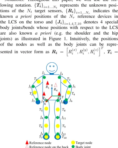
In this paper, only relative localization is addressed. The set of reference nodes is strapped directly into the moving body at some special positions that are independent of the body mobility or gestures (e.g. usually on the torso) to defines a LCS on the human body. Therefore, the positions of the body mounted nodes can be known a priori. Figure 1 illustrates a typical relative localization scenario. The reference nodes are placed on known positions that are not influenced by the body attitude or mobility such as the chest, the back, and the hip. The number of reference devices should not be less than 3 for 2D positioning and 4 for 3D case without any prior knowledge about the target nodes’ positions. Besides, the best placement of reference nodes should be tetrahedral [1], hence, the 4 reference sensors are arranged as follows: one on the chest, one on the back, the two remaining sensors on the hip. For the disposition of the target devices, we avoid attaching these on the joints/bends due to sensors’ possible displacement. Instead, the disposition of target nodes relies on the Xsens MVN system [7].

Notations: Throughout this paper, we will use the fol-lowing notation. {Ti}_i=1...Nt represents the unknown

posi-tions of the Nt target sensors, {Ri}i=1...Nr indicates the known a priori positions of the Nr reference devices in

the LCS on the torso and {Ji}i=1,4,7,10 denotes 4 special

body joints/bends whose positions with respect to the LCS are also known a priori (e.g. the shoulder and the hip joints) as illustrated in Figure 1. Intuitively, the positions of the nodes as well as the body joints can be repre-sented in vector form as Ri =

h R(x)_i , R(y)_i , R(z)_i iT, Ti = 𝑇1 𝑇2 𝑇3 𝑇4 𝑅1 𝑅2 𝑅3 𝑅4 x y z 𝑇5 𝑇6 𝑇7 𝑇8 𝑇9 𝑇10 𝐽1 𝐽2 𝐽4 𝐽5 𝐽3 𝐽7 𝐽6 𝐽8 𝐽9 𝐽10 𝐽11 𝐽12 Reference node

Reference node on the back

Target node Body joint

Figure 1. Relative localization system for BAN. The reference (red) nodes are attached on the torso while the target (yellow) nodes are mounted on the limbs to capture the motion.

h T_i(x), T_i(y), T_i(z)iT, and Ji = h J_i(x), J_i(y), J_i(z)iT. Let ✓ = h T1(x), T (y) 1 , T (z) 1 , . . . , T (x) Nt, T (y) Nt, T (z) Nt iT

be the estimate vec-tor, which consists of unknown parameters. In the same way, we denote the collection of peer-to-peer ranging measurements by the vector ˜d =hd˜11, ˜d12, ˜d13, . . . , ˜d1Nt, ˜d21, . . . , ˜dNrNt

iT

, where ˜dij is the ranging measurement between reference

node i and target node j. So an important point to remember is that dij6= dji,8i 6= j.

As soon as these ranging measurements are determined by the IR-UWB ToA information as proposed in [3], localization algorithms estimate the positions of the target sensors in the LCS. Briefly, given the positions {Ri}_i=1...Nr, some special

joints’ positions (i.e. {Ji}_i=1,4,7,10as in Figure 1) in the LCS

and the ranging information ˜d, the objective is to estimate the vector ✓.

III. LOCALIZATIONALGORITHMS

A. Conventional ML Localization

The ML estimator pays attention to the statistics of the noise sources and maximizes the following likelihood func-tion [1][4]: p⇣d˜|✓⌘= Nr Y i=1 Nt Y j=1 p⇣d˜ij|✓ ⌘ , (1)

where p(·|✓) denotes the conditional probability density func-tion given parameter ✓. And the ML estimator is as follows:

ˆ ✓ = arg max ✓ Nr Y i=1 Nt Y j=1 p⇣d˜ij|✓ ⌘ . (2)

Let consider a simple scenario where the ranging errors are modeled as centered independent Gaussian variables i.e.

˜

dij ⇠ N dij, ij2 , (3)

where dij = Ri!Tj denotes the real distance between the

reference node i and the target node j, then the likelihood function of ✓ takes the form:

p⇣d˜|✓⌘= Nr Y i=1 Nt Y j=1 1 q 2⇡ 2 ij exp 2 4 f ⇣ ✓, ˜d⌘ 2 2 ij 3 5 , (4) f⇣✓, ˜d⌘= ✓ ˜ dij q (Ri Tj)T(Ri Tj) ◆2 . (5)

As a result, the ML has now the formula of the non-linear Weighted Least Squares (WLS) estimator which yields:

ˆ ✓ = arg min ✓ Nr X i=1 Nt X j=1 wijf ⇣ ✓, ˜d⌘, (6)

where wij = 1 2ij plays the role of weight which reflects

the accuracy and the reliability of the measurement ˜dij.

Ac-cordingly, when the measurements have different uncertainties, unreliable ones are down-weighted in the likelihood function

and vice versa, trusted ones are over-weighted. The vector of unknown parameter ✓ in the expression (6) cannot be described in close-form solution. Numerical methods such as Nelder-Mead method [8] are employed to solve this non-linear problem instead.

B. Improved ML Localization

In this part, we propose to adapt the standard ML estimator into the context of BAN.

1) Constrained ML Algorithm: To increase the accuracy, several constraints imposed by the body can provide the ML estimator with extra information. For example, the target node T1 maintains a fixed distance to the shoulder joint J1 as

shown in Figure 2. This constrained localization has been already addressed in [4][5], however, our new constraints are more realistic because of considering both 3D localization and practical placement of the sensors on the body which avoids attaching sensor on the body joints/bends. Without loss of generality, only two sensors T1 and T2 on the left arm

(see Figure 2) are analyzed due to the equivalent roles of the sensors on the arms and legs.

Assuming that all the ranging measurements are indepen-dent and equivalent (i.e. ij = const, 8i, j), the formula (6)

with Nt= 2for the two nodes T1, T2 and Nr= 4becomes:

ˆ ✓ = arg min ✓ 4 X i=1 2 X j=1 ✓ ˜ dij q (Ri Tj)T(Ri Tj) ◆2 , (7) where ✓ = [T1, T2]T = h T₁(x), T₁(y), T₁(z), T₂(x), T₂(y), T₂(z)iT is the estimate vector.

Mathematically, the constraints imposed by the left arm can be formulated as follows: ceq(✓, J1, J2) =  ceq1(✓, J1) ceq2(✓, J2) = 2 6 4 q (T1 J1)T(T1 J1) T1!J1 q (T2 J2)T(T2 J2) T2!J2 3 7 5 = 0, (8)

where ceq(✓, J1, J2)is the matrix composed of the equality

constraints of the target nodes which are determined by their positions on the body.

Note that the position of the left shoulder joint J1 and two

fixed distance T1!J1 , T2!J2 are known a priori whereas

the position of the left elbow joint J2is still unknown. Under

𝑇1 𝑇2 𝑇3 𝑇4 𝐽1 𝐽2 𝐽3 𝐽4 𝑅1 𝑅2 𝑅3 𝑅4 x y z Reference node

Reference node on the back Target node

Body joint Equality constraint Inequality constraint LCS

Figure 2. Constraints in BAN.

normal circumstances, when relying on the placement of target node in Xsens MVN system [7], we have to sacrifice the second constraint (i.e. ceq2(✓, J2) = 0). Therefore, our main

contribution in the constrained algorithm is to gain back this constraint. By using analytic geometry, the position of the left elbow J2can be referred by one of the left shoulder joint J1

and one of the target node T1 as follows:

J2= J1+ ! J2J1 ! T1J1 (T1 J1) . (9)

Substituting J2 in (8) by (9), the constraints now are

inde-pendent of the position of J2. Moreover, we propose to use

also another type of constraint i.e. inequality constraints which have not been investigated in previous studies. For example, in Figure 2, the target node T2cannot reach positions that are 50

centimeters away from the corresponding shoulder joint J1.

However, stricter inequality constraints can be computed by using the following triangle inequalities:

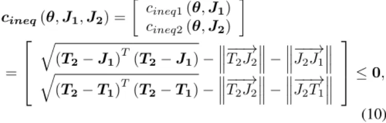
cineq(✓, J1, J2) =  cineq1(✓, J1) cineq2(✓, J2) = 2 6 4 q (T2 J1)T(T2 J1) T2!J2 J2!J1 q (T2 T1)T(T2 T1) T2!J2 J2!T1 3 7 5  0, (10) where cineq(✓, J1, J2) is the matrix that consists of the

inequality constraints of the target nodes which are identified by their positions on the body.

In summary, the constrained localization algorithm leads to find the minimum of constrained nonlinear multivariable function specified by:

ˆ ✓ = arg min ✓ 4 P i=1 2 P j=1 ✓ ˜ dij q (Ri Tj)T(Ri Tj) ◆2 subject to 8 > > > > < > > > > : ceq(✓, J1, J2) = 0 cineq(✓, J1, J2) 0 J2= J1+ ! J2J1 ! T1J1 (T1 J1) . (11) Remind that this optimization problem above is used to estimate the position of 2 target nodes (i.e. ✓ = [T1, T2]T) on

the left arm. For the target nodes on other limbs, the process is equivalent.

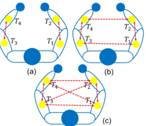
2) Cooperative ML Algorithm: In attempt to improve the precision as much as possible, the features of WSN are investigated and cooperative techniques seem favorable. In conventional localizations, the unknown-position nodes per-form ranging measurements with the known-position nodes whereas cooperative ones enable the communications between unknown-position sensors [2][6]. As shown in Figure 3, the target (yellow) nodes on the arms make measurements with one another to introduce the information redundancies. Our study also considers the effect of the cooperative topology

(a) (b) (c) 𝑇1 𝑇2 𝑇4 𝑇3 𝑇4 𝑇2 𝑇1 𝑇3 𝑇3 𝑇4 𝑇2 𝑇1

Figure 3. (a) Single-link cooperative scenario. (b) Quasi-mesh cooperative scenario. (c) Full-mesh cooperative scenario.

or spacial diversity in the quality of the localization. More particularly, three topologies i.e. single-link (SL), quasi-mesh (QM) and full-mesh (FM) are evaluated.

Firstly, considering the single configuration in Figure 3(a), only target nodes on the same arm are paired to perform the ranging measurements. Sensors on different arms are not allowed to exchange packets in this scenario. The solution for the ML estimation of the positions (of two sensors T1and T2)

in (7) becomes: ˆ ✓ = arg min ✓ h u⇣✓, ˜d⌘+ v⇣✓, ˜dc⌘i, (12) with u⇣✓, ˜d⌘= 4 X i=1 2 X j=1 ✓ ˜ dij q (Ri Tj)T(Ri Tj) ◆2 , (13) and v⇣✓, ˜dc⌘= ✓ ˜ dc12 q (T1 T2)T(T1 T2) ◆2 , (14) where ˜dc

ij denotes the cooperative measurement between the

target node i and the target node j. It can be seen that the likelihood function which is enclosed within square brackets in (12) has a new coefficient i.e. v⇣✓, ˜dc⌘_{in comparison with}

(7). This new coefficient expresses the cooperative localization between unknown nodes (i.e. T1and T2) and provides the ML

estimator with more information.

Next, the spacial diversity is fully exploited by quasi-mesh configuration in Figure 3(b) and full-mesh one in Figure 3(c). In these scenarios, the 4 sensors (i.e. T1, T2, T3, and T4)

on the two arms communicate with one another to form cooperative mesh networks. Consequently, the solution for the ML estimation has the similar form as (12) apart from the cooperative coefficient which becomes:

v⇣✓, ˜dc⌘= X (i,j)2T ✓ ˜ dcij q (Ti Tj)T(Ti Tj) ◆2 , (15) where the estimated vector ✓ = [T1, T2, T3, T4]T and T is the

set of cooperative pairs. In the case of the quasi-mesh topology,

T = {(1, 2), (1, 3), (2, 4), (3, 4)}, while in the case of full-mesh one, T = {(1, 2), (1, 3), (1, 4), (2, 3), (2, 4), (3, 4)}.

Concerning the cooperative approaches, the more cooper-ative measurements, the more information the ML estimator has. However, it is critical to consider the trade-off between extra information and its cost (e.g. over-the-air traffic, power consumption, computational load. . . ). As a result, the cooper-ative techniques should give enough extra information but not largely redundant in order not to increase the complexity of the system. It explains why our cooperative sensor networks con-tain a maximum of four nodes. With these configurations, the most complex ML estimation is limited to a 12-dimensional optimization problem (each target node has three unknown coordinates on the x-axis, y-axis, and z-axis in Cartesian system).

3) Cooperative-cum-Constrained ML Algorithm: In the previous section, both constrained and cooperative localiza-tions have been introduced. Each technique has a complemen-tary strength to the other one. Thus, it is reasonable to merge both algorithms into one to fully exploit the body constraints, the spatial diversity and the measurement redundancies from the BAN in order to achieve superior accuracy. We call this as the Cooperative-cum-Constrained Maximum Likelihood (CCML) algorithm.

IV. SIMULATIONS ANDRESULTS

A. Scenario Description and Simulation Parameters

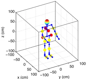
In this section, the framework to evaluate our proposed algo-rithms is presented. Regarding the BAN model, we developed a biomechanical model of a 1.8-meter body as depicted in Figure 4. Four reference nodes are attached on the chest, the back, the left hip, and the right hip to form the LCS whose origin is located at the stomach. Without loss of generality, the two nodes on the left arm are analyzed i.e. node T1 between

the shoulder and the elbow and node T2 between the elbow

and the wrist. In our evaluation framework, the performance of two conventional algorithms (the linear Least Square Error (LSE) and the ML), the family of cooperative techniques (CoopML) with the three different topologies, the constrained scheme (ConML), and the hybrid approaches (i.e. CCML) are evaluated by the Root Mean Square Error (RMSE) and the Geometric Dilution of Precision (GDOP) [1][9] as follows:

RM SE⇣✓ˆ⌘= s E ⇢ ˆ ✓ ✓ 2 , (16) GDOP⇣✓ˆ⌘= q 2 x+ y2+ z2 range , (17)

where ˆ✓ is the estimator of the target or true value ✓ = h

T_i(x), T_i(y), T_i(z)iT. rangedenotes the ranging deviation. x2, 2

y, and z2 represent the mean square errors for the x-axis,

y-axis, and z-axis estimates, respectively. The ranging error is Gaussian noise with ij = range = 5 cm. Therefore,

inde-pendent realizations of ranging measurements are produced to conduct 10,000 simulations of each algorithm.

−100 −50 0 50 100 −100−50 0 50 100 −100 −50 0 50 100 y (cm) x (cm) z (cm)

Figure 4. Sensor deployment in the biomechanical model for relative localization. The reference (red) nodes are attached on the torso to form the LCS while the target (yellow) nodes are mounted on the limbs.

B. Performance Results by Simulations

Figure 5 gives the information about the performance (through RMSE and GDOP) of the analyzed localization al-gorithms for the two nodes T1and T2. The simplest technique

(i.e. LSE) results in the greatest error due to the use of the linear estimator. Next, an improvement in accuracy is provided by the standard non-linear LSE (i.e. the ML) as a result of the consideration of the statistics of noise sources. Then, cooperative scenarios (i.e. CoopML-SL, CoopML-QM and CoopML-FM) reduce the inaccuracy gradually. The more complicated the cooperative network is or the more infor-mation redundancies we provide, the greater accuracy we achieve. A closer look at this figure reveals that the constrained technique (i.e. ConML) has different effects on the different target node’s position estimates. Specifically, the decrease in the GDOP yielded by the body constraints of the T1’s position

estimate is distinctly superior than that of the T2. Furthermore,

in case of the node T2, there exists a slight rise in the RMSE.

This is due to the fact that the position of the node T2(between

the elbow and the wrist) has more degree of freedom than the node T1 (between the shoulder and the elbow). Additionally,

the body constraint related to the node T2depends on the T1’s

position estimate. For this reason, an error in T1’s position

can be magnified and would eventually ruin the T2’s position

estimate. Lastly, the family of hybrid algorithms (i.e. CCML-SL, CCML-QM and CCML-FM) inherits the improvement in accuracy of both constrained and cooperative techniques.

Our results can be compared with other existing works using constrained localization in [4][5]. In the one hand, the constrained ML in [4] results in a relative drop in average RMSE per node of 36.2%–57.3% (depending on the node’s position) compared with the standard ML but this work is limited to 2D positioning. On the other hand, this enhancement is only maximum 17% in [5] on account of the 3D localization

0 5 10 15 20 Algorithm RMSE (cm) LSE ML CoopML −SL CoopML −QM CoopML −FM ConML CCML −SL CCML −QM CCML −FM 0 1 2 3 4 5 6 7 8 GDOP RMSE of node T₁ RMSE of node T₂ GDOP of node T₁ GDOP of node T₂

Figure 5. Relative localization RMSE and GDOP in case of range= 5 cm.

and the reduction in the number of constraints. In contrast, our constrained ML produces the relative enhancement of 32.4% over the ML. Moreover, our hybrid CCML can give more performance (maximum relative improvement of 42.6%). In other words, our CCML algorithm can achieve the minimum absolute RMSE of 4.8 cm in T1’s position estimate and

9.09 cm in T2’s on condition of 5 cm ranging deviation.

V. EXPERIMENTS

This section introduces the real experiments that generate the real measurements in order to validate our algorithms. A. Experimental Setup

The experiments are conducted using DecaWave’s IR-UWB platforms [10] as shown in Figure 6 which have a bandwidth of about 900 MHz centered at 6.5 GHz. Since the ToA is estimated, an antenna delay calibration is required to com-pensate for the system delays between physical timestamp and the signal presence at the antenna. The calibration is performed by placing a couple of DecaWave’s platforms at different distances and adjusting the antenna delay until the range reading given by the device is correct. One platform is fixed, while the other is moved by 10 cm increment toward the static one from a distance of 200 cm to 10 cm. At each separated distance, the calibration is conducted by fine-tuning the antenna delay to get at least 100 fine ranging measurements whose mean is close to the true value (i.e. approximately 1 cm of bias). Two typical configuration modes are used in our experiments i.e. mode 1 employs a low data rate of 110 kbps and long preamble code of 1024 symbols whereas mode 2 uses a high data rate of up to 6.8 Mbps and short code of 128 symbols to save energy [10]. Until the platforms is fine calibrated, these can be used to produce real measurements as input of our analyzed algorithms.

B. Performance Results by Experiments

Firstly, the relation between the antenna delay and the range is exposed in Figure 7. The calibrated delay not only depends on the platform setup but also on the distance. Alternatively,

Figure 6. DecaWave’s IR-UWB EVK1000 kit with UWB antennas.

the first mode has a more stable antenna delay than the second. Thus, the ranging performance of the mode 1 can guarantee higher accuracy in a wide variety of distances while the second can only ensure this accuracy locally in a limited range of distances (i.e. recalibration is required). This is due to the fact that a longer preamble code of mode 1 produces improved range performance and better ToA information [10]. In prac-tice, the same antenna delay is calibrated on all UWB sensors to perform the ranging measurements in every distance. Thus, the mode 1 and an antenna delay of 514.22 ns are adopted to generate real ranging measurements.

Finally, we evaluate our proposed algorithms given the real measurements using DecaWave’s platforms placed on the human body as in Figure 4. For each pair of nodes, 100 ranging measurements are performed to get an average behavior of the algorithms. Their performance are exposed in Figure 8. Ex-pectedly, the body constraints and cooperation between nodes yield improvements in accuracy, which have been observed in the simulations. The order of the performance of the analyzed algorithms coincides with the simulation results. Expectedly, the best accurate position estimate is given by the CCML-FM. Particularly, the RMSE of 2.55 cm and GDOP of 1.038 are recorded in the node T1’s position estimate whereas in the

node T2’s, the performance are degraded to 3.63 cm in RMSE

and 1.341 in GDOP due to high degree of freedom position leading to loose body constraints as discussed.

0 50 100 150 200 513.9 514 514.1 514.2 514.3 514.4 514.5 514.6 Distance (cm) Antenna delay (ns) Mode 1 Mode 2

Figure 7. Calibrated antenna delay for different distances.

0 1 2 3 4 5 6 7 8 9 10 Algorithm RMSE (cm) LSE ML CoopML −SL CoopML −QM CoopML −FM ConML CCML −SL CCML −QM CCML −FM 0 1 2 3 4 5 6 7 8 9 10 GDOP RMSE of node T₁ RMSE of node T₂ GDOP of node T₁ GDOP of node T₂

Figure 8. Relative localization RMSE and GDOP using real measurements.

VI. CONCLUSION

In this paper, we have studied the localization in the context of wireless BAN. By fully exploiting the body constraints and/or cooperative communications, novel algorithms have been presented to increase accuracy performance. These pro-posed algorithms not only outperform various conventional unconstrained and/or non-cooperative techniques (relative de-cline in average RMSE and GDOP per node up to 54% and 56% respectively) but also leave behind other existing works on constrained localization in terms of accuracy and feasibility (our relative improvement of 43% against that of 17% in the work of Hamie et al [5] when considering the relative decrease in average RMSE per node with reference to the standard ML). Lastly, experimental setup shows an accuracy of from 2.55 cm to 3.66 cm depending on the nodes.

REFERENCES

[1] Z. Sahinoglu, S. Gezici, and I. Guvenc, Ultra-wideband Positioning Systems: Theoretical Limits, Ranging Algorithms, and Protocols. Cam-bridge University Press, 2008.

[2] H. Wymeersch, J. Lien, and M. Win, “Cooperative localization in wireless networks,” Proceedings of the IEEE, vol. 97, pp. 427–450, Feb 2009.

[3] S. Gezici, Z. Tian, G. Giannakis, H. Kobayashi, A. Molisch, H. Poor, and Z. Sahinoglu, “Localization via ultra-wideband radios: a look at positioning aspects for future sensor networks,” IEEE Signal Processing Magazine, vol. 22, pp. 70–84, July 2005.

[4] Z. Mekonnen, E. Slottke, H. Luecken, C. Steiner, and A. Wittneben, “Constrained maximum likelihood positioning for uwb based human motion tracking,” in International Conference on Indoor Positioning and Indoor Navigation (IPIN’10), pp. 1–10, Sept 2010.

[5] J. Hamie, B. Denis, and C. Richard, “Constrained decentralized algo-rithm for the relative localization of wearable wireless sensor nodes,” in IEEE Sensors 2012, pp. 1–4, Oct 2012.

[6] N. Patwari, J. Ash, S. Kyperountas, A. Hero, R. Moses, and N. Cor-real, “Locating the nodes: cooperative localization in wireless sensor networks,” IEEE Signal Processing Magazine, vol. 22, pp. 54–69, July 2005.

[7] http://www.xsens.com/.

[8] J. C. Lagarias, J. A. Reeds, M. H. Wright, and P. E. Wright, “Conver-gence properties of the nelder–mead simplex method in low dimensions,” SIAM J. on Optimization, vol. 9, pp. 112–147, May 1998.

[9] J. Zhu, “Calculation of geometric dilution of precision,” Aerospace and Electronic Systems, IEEE Transactions on, vol. 28, pp. 893–895, Jul 1992.

[10] DecaWave Ltd., DW1000 User Manual: How to use, configure and program the DW1000 UWB tranceiver, 2013.