Self adhesion of uncrosslinked polar elastomers

HAL Id: tel-02896761

https://pastel.archives-ouvertes.fr/tel-02896761

Submitted on 23 Oct 2020

HAL is a multi-disciplinary open access

archive for the deposit and dissemination of sci-entific research documents, whether they are pub-lished or not. The documents may come from teaching and research institutions in France or abroad, or from public or private research centers.

L’archive ouverte pluridisciplinaire HAL, est destinée au dépôt et à la diffusion de documents scientifiques de niveau recherche, publiés ou non, émanant des établissements d’enseignement et de recherche français ou étrangers, des laboratoires publics ou privés.

Self adhesion of uncrosslinked polar elastomers

Valentine Hervio

To cite this version:

Valentine Hervio. Self adhesion of uncrosslinked polar elastomers. Material chemistry. Université Paris sciences et lettres, 2019. English. �NNT : 2019PSLET035�. �tel-02896761�

Préparée à l’Ecole Supérieure de Physique et de

Chimie Industrielles de la ville de Paris (ESPCI)

Autohésion d’élastomères polaires non-vulcanisés

Self-adhesion of uncrosslinked polar elastomers

Soutenue par

Valentine HERVIO

Le 19 décembre 2019

Ecole doctorale n° 397

Physique et Chimie des Matériaux

Spécialité

Chimie des matériaux

Composition du jury :

Professeur,

Sorbonne Université Présidente du jury

Pierre-Antoine, ALBOUY Directeur de recherche,

Université Paris-sud Rapporteur

Christophe, DERAIL Professeur,

Université de Pau et des Pays de l’Adour Rapporteur

Annie, BRULET Ingénieure de recherche,

CEA Saclay Examinatrice

Ilias, ILIOPOULOS Directeur de recherche,

ENSAM Examinateur

Costantino, CRETON Directeur de recherche,

Autohésion d’élastomères polaires non-vulcanisés

- Résumé de la thèse en français -

Introduction

Le procédé de fabrication de réservoirs d’hélicoptères implique la superposition de pièces de caoutchoucs non-vulcanisés, et l’ensemble peut être gardé pendant quelques jours à température ambiante avant le cycle de vulcanisation. Une adhérence suffisante entre les différentes couches est nécessaire afin d’empêcher le décollement et l’apparition de défauts. Lors de cette thèse, le matériau d’étude est le caoutchouc nitrile (« Nitrile Butadiene Rubber », NBR), le poly(acrylonitrile-co-butadiene).

Les principaux objectifs de cette thèse sont les suivants :

- Développer une méthode reproductible et discriminante permettant de caractériser les propriétés autohésives de caoutchouc

- Comprendre les phénomènes physico-chimiques régissant l’adhésion, et l’autohésion, de caoutchouc polaires

- Proposer des stratégies afin d’améliorer les performances adhésives du matériau étudié Dans le cadre de cette thèse, le caoutchouc nitrile étudié est fourni par la société Safran sans indication spécifique quant à sa composition ou ses propriétés. Il est comparé à un grade Sigma-Aldrich (« Sigma NBR ») afin de s’assurer que les résultats ne sont pas propres au matériau industriel.

Lors de ce résumé, les matériaux étudiés seront d’abord caractérisés, et la méthode utilisée pour analyser l’autohésion du NBR sera détaillée. Les résultats observés seront expliqués grâce à une étude de la microstructure du matériau. Enfin, certaines stratégies envisagées pour augmenter ces propriétés autohésives seront détaillées.

1. Caractérisation des matériaux

1.1

Détermination du taux d’acrylonitrile

Les élastomères étudiés ont d’abord été caractérisés par DSC (Dynamic Scanning Calorimetry) et ATG (Analyse Thermo-Gravimetrique) afin de déterminer leur taux d’acrylonitrile. Les résultats sont montrés sur la Figure 1.

Figure 1 Courbes de DSC (gauche) et ATG (droite) pour NBR brut (courbes bleues) et pour NBR-SA (courbes rouges)

En s’appuyant sur les travaux de Sircar [1], il est possible d’estimer le taux d’ACN dans chaque élastomère pour les deux matériaux :

Matériau Taux d’ACN Tg (°C)

Raw NBR 32 +/- 2% -31

Sigma NBR 43 +/- 1% -14

Tableau 1 Propriétés des NBR étudiés

1.2

Propriétés mécaniques

Les propriétés mécaniques ont été étudiées dans le régime linéaire, et l’utilisation de l’équivalence temps-température (TTS) a permis de tracer une courbe maîtresse à température ambiante (Figure 2).

Les propriétés mécaniques en grande déformation ont également été étudiées en effectuant des tests en traction uniaxiale (Figure 3), et le module d’Young a été estimé à 0.5 +/- 0.1MPa (Ɛ = 0.017 ).

Figure 2 Courbe maîtresse du NBR (extrude) à To=25°C Figure 3 Traction uniaxiale sur NBR (extrudé)

-0.8 -0.7 -0.6 -0.5 -0.4 -0.3 -0.2 Heatfl ow ( W /g) 80 40 0 -40 -80 Temperature (°C) -14°C -31°C 80 60 40 20 0 W e ight ( % ) 800 600 400 200 Temperature (°C) 5.2% 8.4% Raw NBR Sigma NBR 1.4 1.2 1.0 0.8 0.6 0.4 0.2 Tan δ 10-5 10-3 10-1 101 103 aTf (Hz) 103 104 105 106 107 bT G ',G '' (P a) 0.10 0.08 0.06 0.04 0.02 0.00 Str e ss ( M Pa) 16 14 12 10 8 6 4 2 0 Strain (ε)

1.3

Caractérisation des propriétés adhésives

Afin de caractériser les propriétés adhésives des élastomères, la méthode du Probe-Tack (bien détaillée dans la littérature [2]) a été le point de départ.

Figure 4 Machine du Probe-tack

Lors de ces essais types, un poinçon de 9.7mm de diamètre est mis en contact, à 1MPa, avec un adhésif déposé sur une plaque de verre. Après un certain temps de contact noté tc, le poinçon se

rétracte et le couple force-déplacement nécessaire pour le décollement est mesuré. Un miroir orienté à 45° permet d’observer les mécanismes de décollement à l’interface et de vérifier que le poinçon et la plaque sont bien alignés.

Lors de l’étape de décollement, la contrainte σ et la déformation Ɛ sont calculées à partir de la force F et du déplacement l :

=

= − ℎ

ℎ

Avec ho l’épaisseur initiale du système adhésive et A l’aire de contact. L’énergie d’adhésion Wadh

(J/m²) est ensuite calculée telle que :

= ℎ

Ɛ

Cette méthode a été largement utilisée pour étudier l’adhésion de couche fine de matériaux mous types PSAs sur du verre [3][4][5].

Dans le cadre de cette thèse, nous avons mesuré l’adhésion entre une fine couche (~10microns) de NBR déposée sur la plaque de verre, et une couche plus épaisse (~500microns) collée sur le poinçon. La méthode du Probe-tack est utilisée pour étudier des temps de contacts de l’ordre de quelques dizaines de secondes (500 secondes maximum). L’autohésion du NBR mesurée pour de tels temps de contact étant très faible (Wadh ~ 30J/m² pour 500 secondes), une nouvelle méthodologie d’essai a été définie. Celle-ci permet de séparer l’étape de formation du contact et

Figure 5 Illustration du poids appliqué (haut gauche), des échantillons (bas gauche) et du montage expérimental (droite)

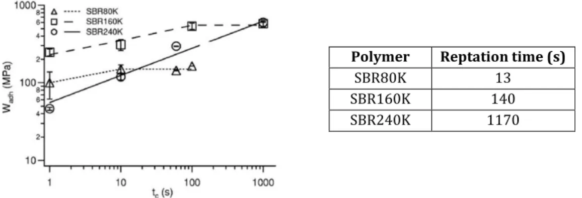
Les propriétés autohésives du NBR augmentent faiblement avec le temps de contact. Contrairement à ce qui a été trouvé sur des matériaux apolaires type SBR (Styrene Butadiene Rubber) dans les études de Schach [4][6], il n’y a ici aucune corrélation entre l’évolution des propriétés adhésives avec le temps, et les temps caractéristiques de relaxation mesurés en rhéologie linéaire. Par ailleurs, aucun plateau n’est observé aux longs temps de contact.

Figure 6 Evolution des propriétés autohésives (courbe contrainte-déformation) du NBR en fonction du temps de contact

Figure 7 Evolution de l’énergie d’autohésion Wadh du NBR

avec le temps de contact

2. NBR comme matériau supramoléculaire

2.1

Observation d’une microstructure

Ces faibles propriétés autohésives sont liées à l’existence d’une structure supramoléculaire au sein du matériau. En effet, deux états sont comparés : directement après extrusion (« NBR-ext »), puis après solubilisation et séchage lent (« NBR-solub »). Ces matériaux s’avèrent être complètement différents, notamment en rhéologie linéaire (voir Figure 8) : là ou NBR-ext s’écoule

0.6 0.5 0.4 0.3 0.2 0.1 0.0 St re ss (MPa ) 0.6 0.4 0.2 0.0 Strain (ε) 24h 42h 96h 168h 60 50 40 30 20 10 0 W adh ( J/m² ) 0.1 1 10 100 1000 contact time (h)

(dans le sens où un temps terminal de relaxation est mesurable, tan δ >1), NBR-solub se comporte comme un gel physique et le facteur de perte reste supérieur à 1 même aux faibles fréquences.

Figure 8 Propriétés rhéologiques linéaires pour NBR-ext (rouge) et NBR-solub (noir). Gauche: modules de stockage G' et de perte G''. Droite: Facteur de perte

Des études en diffraction de rayons-X (SAXS) ainsi qu’en AFM (Atomic Force Microscopy) ont notamment pu confirmer l’existence d’une structuration au sein du matériau. En effet, la Figure 9 montre l’existence de deux structures lamellaires à q=0.1366 et q=0.1458 A-1_{, correspondant}

respectivement à des tailles de 4.6 et 4.3 nm. Sur l’échantillon extrudé, cette structure est détruite et un pic amorphe (lié à une structure mal définie) est observé proche de 0.2A-1_{. Cette structure}

réapparait lorsque l’échantillon extrudé NBR-ext est laissé pendant plusieurs mois à température ambiante (voir Figure 10).

Figure 9 Courbes de SAXS sur du NBR fraichement extrudé et du NBR

solubilisé Figure 10 Effet du vieillissement sur la microstructure observée en SAXS 104 2 4 6 8 105 2 4 6 8 106 2

G',

G'' (P

a)

a

f (Hz)

Tan

δ

a

f (Hz)

Profile d’intensité

Figure 11 Observation de la structure lamellaire en AFM

2.2

Utilisation de la RMN pour comprendre cette

microstructure

Une étude détaillée en RMN 1_{H en solution nous a permis d’estimer la statistique du copolymère}

étudié. Il a été trouvé que le monomère acrylonitrile existe seulement en alternance avec des unités butadiènes, alors que le butadiène peut exister sous forme de blocks. Ainsi, il est suggéré que le matériau initialement supposé statistique est, en réalité, un copolymère à block avec des

blocks de polybutadiène, et des blocks avec des unités butadiène et acrylonitrile alternées. Une chaîne de NBR est schématisée en Figure 12.

Figure 12 Schéma illustrant une chaîne de NBR

Les monomères acrylonitrile et butadiène étant fortement immiscible, les chaînes vont s’organiser afin de limiter ce coût enthalpique, et ainsi former des lamelles (Figure 13).

Figure 13 Organisation du NBR en lamelles

Des interactions intramoléculaires fortes entre groupement nitrile, ainsi que l’immiscibilité des blocks, empêche la migration de chaînes et peut ainsi expliquer le comportement rhéologique observé et les faibles propriétés autohésives mesurées.

3. Stratégies proposées pour augmenter propriétés

autohésives du NBR

3.1

Effet de la température

L’effet de la température a été étudié entre 40 et 120°C. Il semblerait que la destruction à haute température de l’une des structures lamellaires observées en SAXS (Figure 14) permet la migration de chaînes polymères à l’interface, et donc une nette augmentation des propriétés autohésives (Figure 15).

Figure 14 Observation par SAXS de l’évolution de la

structure du NBR en fonction de la température Figure 15 Evolution des propriétés autohésives du NBR en fonction de la température de contact

2 4 6 8 0.1 2 4 6 8 1 2 Intensi ty ( cm-1) 3 4 5 6 0.1 2 3 4 5 6 1 2 q(A-1) 20°C 85°C 500 400 300 200 100 0 W a dh (J/m²) 120 100 80 60 40 20 0 T(°C)

tackifiante a été ajoutée au NBR à l’aide d’une extrudeuse. Deux résines, l’une phénolique (polaire) et l’autre hydrocarbonée (apolaire), ont été étudiées, à différentes concentrations. Pendant ces travaux, deux régimes ont été examinés : les faibles (3%) et fortes (>10%) concentrations. Des temps de contact allant de 1 heure à plusieurs jours ont été étudiés.

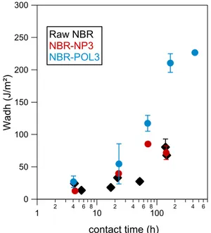
Les travaux réalisés ont permis de montrer que pour les faibles concentrations, la nature chimique de la résine est clef. En effet, aux longs temps de contact, une nette amélioration des propriétés auto-hésives du NBR est observée avec l’ajout de résine phénolique (voir Figure 16). Un mécanisme, reposant sur la capacité des molécules polaires à perturber les interactions intermoléculaires C≡N, est proposé pour expliquer une telle augmentation.

Figure 16 Evolution de l'énergie d'adhésion Wadh en fonction du temps de contact, pour les 3 matériaux considérés

A plus forte concentration (10 et 20%), la nature chimique de la résine tackifiante influence peu les propriétés autohésives du NBR. Une nette amélioration est cependant observée, aux faibles temps de contact, lorsque la concentration est augmentée de 10 à 20%. Des caractérisations mécaniques sont effectuées afin de discuter ces résultats. Par ailleurs, des analyses en SAXS montrent que l’ajout de telles concentrations perturbe fortement la microstructure du NBR. Il est suggéré que, pour des considérations de coût entropique, à forte concentration la résine apolaire migre dans les lamelles polaires et perturbe également les liaisons intermoléculaires. L’évolution de ces structures dans le temps est discutée, ainsi que l’influence de celle-ci sur les propriétés auto-hésives des matériaux.

Ainsi, le choix de la nature ainsi que de la concentration de la résine dépend fortement de l’application souhaitée. En effet, si un fort collant est nécessaire à faible temps de contact, alors il semble nécessaire d’introduire 20% de résine, et la nature chimique de celle-ci n’a que peu d’influence. Au contraire, si le collant est nécessaire aux temps longs, alors seulement 3% de résine peut suffire, et il est alors nécessaire de s’orienter vers une résine polaire. La Figure 17 montre l’effet de la concentration de chaque résine, pour deux temps de contact considérés.

300 250 200 150 100 50 0 W adh ( J/ m ²) 1 2 4 6 810 2 4 6 8100 2 4 6 contact time (h) Raw NBR NBR-NP3 NBR-POL3

Figure 17 Evolution de l'énergie d'adhésion en fonction de la quantité de résine tackifiante introduite, pour les deux types de résine. Gauche: temps de contact=5.5 heures. Droite: temps de contact = 7 jours

3.3

Avivage par solvant

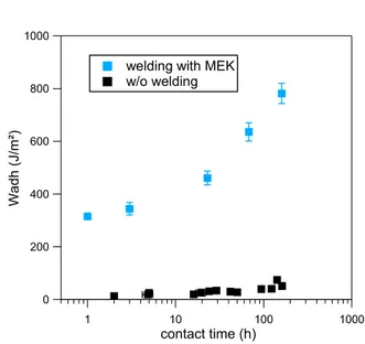
Cette stratégie est inspirée du procédé industriel, et consiste à utiliser l’ajout de solvant à l’interface afin de la souder et de permettre une adhésion forte entre les deux couches non vulcanisées. La Figure 18 compare les propriétés autohésives du NBR brut sans et avec avivage (avec du butanone).

Figure 18 Influence de l’avivage sur les propriétés autohésives du NBR pour tc=24h

Figure 19 Evolution de l'énergie d'autohésion en fonction du temps de contact pour NBR avec et sans avivage au MEK

L’énergie d’adhésion mesurée est significativement augmentée (Wadh= 470Jm² vs 30J/m² sans

avivage pour 24 heures de contact). En effet, l’ajout de solvant permet non seulement d’assurer un contact parfait (aire de contact maximale) entre les deux surfaces, mais surtout de perturber la structure lamellaire présente en surface des couches. Ainsi, la migration des chaînes polymères est facilitée et l’interface renforcée. Une forte dissipation d’énergie est possible grâce à la formation de fibrilles. La Figure 19 montre l’évolution de l’énergie d’autohésion Wadh pour

différents temps de contact après avivage au MEK.

300 250 200 150 100 50 0 Wa dh (J/m ²) 50 40 30 20 10 0 Tackifier content (%) pure NBR NBR-NP NBR-POL tc= 5.5hours 20% 300 250 200 150 100 50 0 Wa dh (J/m ²) 50 40 30 20 10 0 Tackifier content (%) tc= 7 days pure NBR NBR-NP NBR-POL 3% 1.0 0.8 0.6 0.4 0.2 0.0 St re ss (MPa ) 8 6 4 2 0 Strain (ε)

welding with MEK w/o welding 1000 800 600 400 200 0 Wa dh (J /m²) 1 10 100 1000 contact time (h) welding with MEK w/o welding

douze solvants, pour un temps de contact de 3 heures.

L’influence de la qualité du solvant pour le NBR, estimé par des mesures de gonflement, a d’abord été investiguée. Cette étude nous a montré que les meilleurs solvants pour le polymère n’étaient pas nécessairement les meilleurs solvants pour l’avivage. D’autres paramètres tels que la température d’ébullition, l’affinité spécifique pour un monomère de ce copolymère à multi-blocks (acrylonitrile ou butadiène) et le moment dipolaire ont été étudiés. Les solvants avec des moments dipolaires élevés et présentant des températures d’ébullition intermédiaires (50°C < Teb < 150°C

dans cette étude) semblent être optimaux. Cependant, malgré une connaissance approfondie du copolymère à block NBR, et de sa microstructure, prévoir exactement l’influence d’un solvant sur les propriétés d’autohésion de cet élastomère reste délicat.

4. Conclusion

Lors de cette thèse, une adaptation de la méthode du Probe-Tack a été proposée afin de caractériser les propriétés autohésives de matériaux mous pour de faibles pression et longs temps de contact. Cette nouvelle méthodologie permet de dissocier les étapes de formation du contact, et de décollement, particulièrement pertinent pour étudier l’influence de la température sur ces propriétés d’interface.

Il est montré que les propriétés autohésives du NBR sont faibles et évoluent peu avec le temps de contact. Cette particularité est attribuée à la présence de lamelles de tailles nanométriques dans les échantillons. La formation de cette microstructure est due à la statistique du matériau étudié qui n’est non pas statistique mais à block, avec des blocks de monomère butadiène et des blocks formés d’unités butadiène et acrylonitrile alternées. La très faible miscibilité de ces deux monomères, ainsi que la présence d’interaction intermoléculaire C≡N entre groupements nitriles, rend la diffusion de chaînes à l’interface thermodynamiquement très peu favorable.

Plusieurs méthodes ont été proposées afin d’améliorer ces propriétés autohésives. Le choix d’une méthode plutôt que l’autre dépend fortement de l’application considérée et notamment du temps de contact qu’il est possible d’atteindre. Les mécanismes par lesquels chaque méthode (température, ajout d’une résine tackifiante, avivage par solvant) est efficace sont étudiés et débattus en s’appuyant sur des essais de caractérisation mécanique, sur des observations microscopiques, ainsi que sur des analyses de diffraction en rayon X.

Enfin, l’ajout de particules de PVC envisagé afin de renforcer mécaniquement le matériau NBR. Il est montré que cette molécule polaire change considérablement les propriétés autohésives de l’élastomère, et l’effet de la résine tackifiante est plus complexe à expliquer.

5. References

[1] R. Schach, Y. Tran, A. Menelle, and C. Creton, “Role of chain interpenetration in the adhesion between immiscible polymer melts,” Macromolecules, vol. 40, no. 17, pp. 6325–6332, 2007. [2] H. Lakrout and P. Sergot, “Direct Observation of Cavitation and Fibrillation in a Probe Tack

Experiment on Model Acrylic Pressure- Sensitive-Adhesives,” no. 1999, pp. 37–41.

[3] C. Creton and H. Lakrout, “Micromechanics of flat-probe adhesion tests of soft viscoelastic polymer films,” J. Polym. Sci. Part B Polym. Phys., vol. 38, no. 7, pp. 965–979, 2000.

[4] C. Creton and R. Schach, “Adhesion at interfaces between highly entangled polymer melts,”

J. Rheol. (N. Y. N. Y)., vol. 52, no. 3, pp. 749–767, 2008.

[5] F. Tanguy, L. U. Pierre, and E. T. Marie, “Debonding mechanisms of soft adhesives : toward adhesives with a gradient in viscoelasticity Debonding Mechanisms of Soft Adhesives : Toward Adhesives with a Gradient in Viscoelasticity,” 2014.

List of abbreviations

GENERAL INTRODUCTION

……….…….1

CHAPTER 1 – From molecular dynamics to strong self-adhesion properties

1 Elastomers and their molecular dynamics ... 8

1.1 Processing and key properties of elastomers ... 8

1.2 Physics of rubber elasticity ... 9

1.3 Dynamics of viscoelastic materials ... 13

2 Introduction to the adhesion of soft materials ... 16

2.1 Adhesive performance of soft materials ... 17

2.2 Macroscopic characterization of adhesion ... 18

2.3 Comments ... 19

3 Formation of a strong interface ... 19

3.1 Molecular theories... 19

3.2 Formation of intimate contact ... 20

3.3 Polymer interfaces between polymer melts ... 23

4 Energy dissipation as key to boost adhesion strength ... 29

4.1 Introduction to debonding in soft materials ... 30

4.2 Predicting debonding mechanisms from linear rheology ... 31

4.3 Non-linear fibrillation ... 33

4.4 End of the story: final detachment ... 34

5 Effect of molar mass on adhesion ... 34

6 Nitrile Butadiene Rubber (NBR) ... 35

6.1 Introduction to poly(acrylonitrile-co-butadiene) ... 35

6.2 Adhesion and self-adhesion properties of NBR ... 38

7 Conclusion ... 40

CHAPTER 2 – Characterization of nitrile rubber

1. Material characterizations ... 49

1.1 Average molecular weight ... 49

1.2 Acrylonitrile content ... 49

2. Characterization of mechanical properties... 52

2.1 Linear rheology... 52

2.1 Uniaxial tensile tests ... 56

3. Characterization of adhesion properties ... 57

3.1 Choice of the characterization method ... 57

3.2 Probe-tack tests ... 58

3.3 Samples’ preparation ... 61

3.4 Self-adhesion properties ... 62

4. Conclusions and discussion ... 65

4.1 Discussion ... 65

4.2 Conclusions ... 68

1. Supramolecular behavior of NBR ... 73

1.1. Ageing of the materials at room temperature ... 73

1.2. Dissolution of NBR in a solvent to accelerate ageing process ... 77

1.3. Conclusions ... 79

2. Study of structure formation in NBR ... 80

2.1. Literature ... 80

2.2. X-Ray Scattering ... 82

2.3. Atomic Force Microscopy ... 88

2.4. Transmission Electron Microscopy ... 91

2.5. 1H NMR study ... 91

2.6. Conclusions and discussion ... 93

3. “Self”-adhesion properties ... 94

3.1. Literature on block copolymers... 94

3.2. Influence of NBR structure on its self-adhesion properties ... 97

3.3. Self-adhesion properties of freshly extruded NBR ... 101

4. Conclusions ... 103

CHAPTER 4 – Influence of tackifiers on the self-adhesion of nitrile rubber

1. Literature on the blending of tackifiers ... 109

1.1. General picture ... 109

1.2. Influence of the nature and the amount of tackifier ... 109

1.3. Additives in phase-separated materials ... 111

1.4. Conclusion and discussion ... 112

2. Introduction ... 113

3. Blending of 3% tackifier in NBR ... 115

3.2. Bulk properties and structure ... 118

3.3. Conclusion and discussion ... 120

4. Blending of a high tackifier content in NBR ... 122

4.1. Self-adhesion properties ... 122

4.2. Properties of the high concentration blends ... 126

5. Conclusion ... 132

1. Introduction to solvent welding ... 137

1.1. Literature ... 137

1.2. Methods ... 138

2. Influence of solvent welding on the adhesion and adhesion of NBR ... 140

2.1. Adhesion of welded NBR on glass ... 140

2.2. Self-adhesion of welded NBR ... 140

3. Influence of the solvent ... 144

3.1. Presentation of the different solvents ... 144

3.2. Influence of solvent’s quality for the polymer ... 144

3.3. Importance of solvents’ vapor pressure ... 147

3.4. Site-specific swelling for welding ... 148

3.5. Influence of the dipole moment ... 149

3.6. Conclusions ... 150

4. Effect of microstructure on solvent-welded NBR ... 151

4.1. Introduction ... 151

4.2. Influence of microstructure of self-adhesion of NBR ... 151

4.3. Conclusion ... 153

5. Influence of drying conditions ... 154

5.1. Effect on the self-adhesion properties ... 154

5.2. Investigations ... 155

5.3. Discussion ... 158

6. Conclusions ... 159

CHAPTER 6 – First insights into PVC-blended nitrile rubbers (NBR/PVC)

1. Literature: Blending of PVC in NBR ... 165

1.1. Introduction to NBR/PVC ... 165

1.2. Composition-dependent properties... 165

1.3. Nanoscale heterogeneity ... 166

2. Samples preparation and characterization ... 167

2.1. Blends preparation ... 167

2.2. Mechanical properties of NBR/PVC blends ... 168

2.3. Structural organization ... 170

3. Self-adhesion properties of NBR/PVC ... 173

3.1. Samples’ preparation ... 173

3.2. Influence of contact time on the self-adhesion properties of NBR/PVC blends ... 173

3.3. Solvent welding to enhance self-adhesion properties ... 175

3.4. Conclusions and discussion ... 177

4. Addition of tackifiers to NBR/PVC ... 178

4.1. Self-adhesion properties of NBR/PVC with tackifiers ... 179

4.2. Mechanical properties of NBR/PVC with tackifiers ... 181

4.3. Discussion ... 183

5. General conclusions and discussion ... 184

6. References ... 185

CONCLUSIONS AND PERSPECTIVES

………..………187

ANNEXES

1. Characterizations of the materials ... 193

1.1 NMR of NBR-SA ... 193

1.2 SEC curve of raw NBR in toluene ... 194

1.3 Method to check concentration of PVC in blends ... 194

2. Determination of NBR linear regime ... 195

3. Structure observation ... 196

3.1 SAXS of Tackifier + 3%: solubilized and aged ... 193

3.2 SAXS- Drying conditions ... 194

List of abbreviations

NBR Nitrile Butadiene Rubber

SBR Styrene Butadiene Rubber

Tg Glass Transition Temperature

Phr Parts per hundred of rubber

PB Polybutadiene

MEK Methyl Ethyl Ketone = Butanone

PSA Pressure Sensitive Adhesives

ACN Acrylonitrile

DSC Dynamic Scanning Calorimetry

1

- GENERAL INTRODUCTION -

1. Industrial interest and fabrication process

Safran produces different types of equipment for the aerospace industry, and among them helicopter fuel tanks. Because of its application, very well defined specifications are set and key requirements exist. First, the product, and therefore the used materials, must be resistant enough to withstand the mechanical stresses (induced by vibrations and fluid’s movement) present in a helicopter. Moreover, fuel tanks have to be flexible, because of the need to optimize space in the aircraft. Indeed, in a helicopter, the tanks occupy all the space free of use after seats and equipment. Last but not least, the tank has to be lightweight and fuel-resistant, which implies specific properties regarding the used materials. For all the above reasons, Safran creates a very complex assembly with different polymer layers, and especially polar elastomers. To understand this work’s problematics well, it is necessary to focus on the fuel tanks’ fabrication process.

Materials storage

The elastomers used are provided by an external supplier by batches of several hundreds of kilograms and are then kept in a storehouse inside the factory. The storage temperature is that of the storehouse, and can possibly vary from 0°C in the winter to up to 40°C in the summer. Materials are used in the year following their reception.

Materials processing

The rubbers are first compounded through an internal mixer and then calendered at 80°C, where up to fifteen different additives such as anti-oxidants, plasticizers, fillers and tackifiers are blended. A second calendering at 100°C is performed to reach thinner sheets, with a final thickness of about 400 micrometers. Right after the calendering process, the sheets are enrolled, between two protective plastic liners to avoid any adhesion between the different layers. The sheets are then kept aside, at room temperature, until used for fuel tank fabrication.

Fuel tank fabrication

The size and the geometry of each fuel tank is specific for a given helicopter. To produce a tank, an adequate metallic mold is needed (see Figure 1). The process consists in overlaying different sheets of materials, either rubber or coated fabric, in a very accurate way. In between each layer, the surfaces are scrubbed with a rag impregnated with solvent. Once the assembly is completed, the fuel tank is covered with a vacuum bag and is placed in the autoclave for the vulcanization cycle. During this vulcanization step, the elastomer chains are crosslinked with sulphur.

GENERAL INTRODUCTION

2

Figure 1 Pictures of a fuel tank mold (left) and of a helicopter fuel tank (right)

Changes in materials (rubber + additives) as well as changes in the processing conditions can modify the contact strength between the unvulcanized layers. In the industry, it is important to have a fine understanding of the adhesion mechanisms to be able to adapt the bonding strategy.

2. Thesis challenges

One of the polar elastomers used by Safran is the poly(acrylonitrile-co-butadiene), most commonly called “nitrile rubber” (NBR). The present study is focused on this material. As the industrial process is very complex, representative (and simplified) contact conditions will be determined to characterize the adhesion properties of such materials.

Self-adhesion characterization method

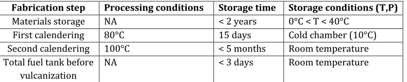
The goal is to develop a methodology to reproducibly and quantitatively characterize self-adhesion properties of uncrosslinked nitrile rubbers. This method must be as relevant as possible for the industrial process. Therefore, the different time scales as well as the processing and storage conditions need to be taken into account for the method development:

Fabrication step Processing conditions Storage time Storage conditions (T,P)

Materials storage NA < 2 years 0°C < T < 40°C

First calendering 80°C 15 days Cold chamber (10°C)

Second calendering 100°C < 5 months Room temperature

Total fuel tank before vulcanization

NA < 3 days Room temperature

Table 1 Different processing and storage conditions for each fabrication step

One of the method’s key requirements is to confirm that the experimental observations noticed by the workers during the manufacturing process are well reproduced by the testing method.

Scientific challenge

To the best of our knowledge, the adhesion and self-adhesion of unvulcanized polar elastomers have not been reported in the literature. Although the inter-diffusion mechanisms of polymer chains at the interface is well documented (see Chapter 2), all these studies have focused on non-polar, linear and monodisperse materials. Yet during this work, an industrial grade of polymer is studied, with additional complexities such as a poorly controlled molar mass distribution and molecular architecture. The goal of this project is to determine the main materials and processing parameters influencing the self-adhesion of a given polar polymer, and to understand the physics and chemical process implied.

3

3. Scope of the manuscript

A general overview on elastomers and their dynamic properties, as well as an introduction to their adhesion, and self-adhesion, properties is presented in Chapter 1. The rest of the manuscript follows the thesis’ chronology. In chapter 2, the methods to characterize both thermal and mechanical properties are presented and used to measure nitrile rubber’s behavior. The material’s self-adhesion properties are first characterized using a classical Probe-tack device, and a new protocol, better adapted for this material is then developed. Chapter 3 focuses on the development of a microstructure in the bulk, which explains the particular behaviors probed in Chapter 2. Several characterization techniques are used to observe and understand the formation of such organization. Chapter 3 also gives an insight on the relation between structure and adhesion properties. In the chapters that follow, two strategies to enhance the rubbers’ self-adhesion properties are exposed, and explained in light of the structure-property scheme exposed in Chapter 3. A first strategy consists in blending small molecules called “tackifiers” inside NBR, and is detailed in Chapter 4. The use of solvent to weld the interface is then thoroughly studied in Chapter 5. Finally, poly(vinyl chloride) particles are blended into NBR and its influence on the structure and the self-adhesion properties are studied in Chapter 6.

In addition to the general literature on elastomers and adhesion presented in Chapter 2, appropriate state-of-the art and relevant references are detailed in the beginning of each chapter to comprehend the new concepts needed to analyze the results.

5

- CHAPTER 1 -

FROM MOLECULAR DYNAMICS TO STRONG

SELF-ADHESION PROPERTIES

The objective of this chapter is to provide the reader with the thesis’ key notions, and to set its general framework.

A simple physical analysis of elastomers’ elasticity and viscoelasticity is first presented, and the dynamics of their melts are analyzed in light of rheological measurements. The relaxation processes introduced are key to understand the interdiffusion responsible for the formation of a strong interface between two polymer melts. The extent of energy dissipation during the debonding process, and failure mechanisms are then discussed. The effect of molecular weight as a trade-off between the development of a strong interface and the bulk dissipation between debonding is presented. Finally, an introduction on Nitrile Butadiene Rubber (NBR)’s processing and on its adhesion properties is presented.

6

1

Elastomers and their molecular dynamics ... 8

1.1 Processing and key properties of elastomers ... 8

1.1.1 Formulation and shaping of elastomer ... 8 1.1.2 Basics of elastomers mechanical properties... 8

1.2 Physics of rubber elasticity ... 9

1.2.1 Thermodynamics of rubber (entropic elasticity) ... 10 1.2.2 Rubber elasticity in a crosslinked network ... 11 1.2.3 Entangled rubber elasticity ... 12 1.2.4 Strain hardening ... 12

1.3 Dynamics of viscoelastic materials ... 13

1.3.1 Introduction to linear viscoelasticity ... 13 1.3.2 Unentangled polymer dynamics (M<Me) ... 14

1.3.3 Entangled polymer dynamics (M>2Me) ... 15

1.3.4 Rheology of entangled polymer melts ... 15

2

Introduction to the adhesion of soft materials ... 16

2.1 Adhesive performance of soft materials ... 17

2.1.1 Pressure Sensitive Adhesives (PSA) as soft adhering materials ... 17 2.1.2 Introduction to the tack behavior of elastomers ... 17

2.2 Macroscopic characterization of adhesion ... 18 2.3 Comments ... 19

3

Formation of a strong interface ... 19

3.1 Molecular theories... 19 3.2 Formation of intimate contact ... 19

3.2.1 Cavitation ... 20 3.2.2 Parameters influencing microscopic contact ... 20 3.2.3 Adhesion on glass ... 21 3.2.4 Comments ... 22

3.3 Polymer interfaces between polymer melts ... 22

3.3.1 Methods to observe motions ... 22 3.3.2 Adhesion of immiscible polymers: a thermodynamic study ... 24 3.3.3 Self-adhesion of polymers: kinetics ... 26 3.3.4 Conclusion and comments ... 29

4

Energy dissipation as key to boost adhesion strength ... 30

4.1 Introduction to debonding in soft materials ... 30

4.1.1 Need for dissipation ... 30 4.1.2 Types of cavities growth ... 30

4.2 Predicting debonding mechanisms from linear rheology ... 31

4.2.1 From materials elastic behavior... 31 4.2.2 Considering viscoelastic dissipation ... 32

4.3 Non-linear fibrillation ... 33 4.4 End of the story: final detachment ... 34

5

Effect of molar mass on adhesion ... 34

5.1.1 Influence of molar mass on interface dynamics ... 34 5.1.2 Influence of molar mass on the green strength ... 35 5.1.3 Trade-off between tack and green strength ... 35

7

6

Nitrile Butadiene Rubber (NBR) ... 36

6.1 Introduction to poly(acrylonitrile-co-butadiene) ... 36

6.1.1 Presentation ... 36 6.1.2 Manufacturing ... 36

6.2 Adhesion and self-adhesion properties of NBR ... 38

6.2.1 Adhesion of NBR to other materials ... 38 6.2.2 Self-adhesion of NBR ... 39

7

Conclusion ... 40

8

References ... 41

CHAPTER 1 - 1. Elastomers and their molecular dynamics

8

1 Elastomers and their molecular dynamics

Polymers are large molecules, macromolecules, composed of many repeating subunits called “monomers”. Elastomers (rubbers) are a specific type of polymer, with very weak intermolecular forces, used at temperatures well above that of their glass transition. Crosslinking of the rubbery chains are needed for the material to show its great mechanical properties. They are stretchable to high strains in a reversible way, and have a low Young’s modulus (~MPa). During this first part, an introduction to rubbers’ great elasticity and a rapid study of their dynamics in melt is proposed.

1.1 Processing and key properties of elastomers

In the rubber industry, manufacturers themselves prepare the blends on specific tools and therefore control all the processing parameters, as well as the formulation [1].

1.1.1 Formulation and shaping of elastomer

i. Formulation

The main component is, of course, the uncrosslinked rubber itself. It is either natural rubber, or synthetized by polymerization of oil-based monomers (ethylene, propylene, butadiene, styrene...). The polymerization technique as well as the used catalysts determine the structure and the molecular mass of the polymer. Different additives are blended, among which: fillers, plasticizers, stabilizers and vulcanizing agents. The nature and the amount of each additive is well controlled and optimized to satisfy the specifications.

Additives Role

Vulcanizing agents Forming the three dimensional elastic network

Fillers Reinforcement and/or dilution

Plasticizers Processing agent, flexibility, glass transition temperature Stabilizers Protection against aging, heat, UV, ozone…

Others Flame retardant, foams, adhesion, colors…

Table 1 The role of the most common additives blended in rubber Blending is performed in two steps:

- On an internal mixer to add fillers and oils. These tools operate discontinuously. During this step, temperature can rise up to 180°C due to viscous heating

- On cylinder mixers, also called “calenders”, at a much lower temperature to blend the vulcanizing agents without risking a premature crosslinking

ii. Shaping

Once the blend is ready, it is shaped using polymer molding classical techniques: injection, extrusion or compression. In the case of tires- and helicopter fuel tanks- shaping consists in overlaying the bands of raw (unvulcanized) rubber bands, and the structure relies on each layers’ specific function and positioning. The assembly is then vulcanized in appropriate presses.

1.1.2 Basics of elastomers mechanical properties

i. Vulcanization

Vulcanization is the final step of the fabrication process. It consists in fixing the three-dimensional structure through chemically crosslinking the polymer chains. The reactions are thermally triggered. The vulcanized rubber cannot be modified afterwards and heating leads to its pyrolysis

9

rather than its fusion. There are mainly two types of chemical agents for vulcanization: peroxides and sulfur compounds [2][3]. Sulfur bridging of polymer chains is illustrated in Figure 1.

Crosslinking point

Figure 1 Vulcanization of polymer chains through sulfur bridges (crosslinking points) Elastomers are used in this crosslinked state, which is referred to as “cured”.

ii. Mechanical properties

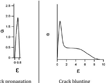
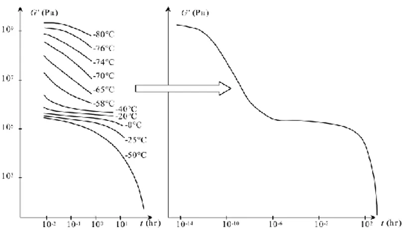
Elastomers are a specific kind of polymer, with very weak intermolecular forces, used at temperatures well above that of their glass transition (which is lower than 0°C). Their modulus drops of several orders of magnitude (from GPa to MPa) at this specific temperature (see Figure 2) and vulcanization prevents their flow at very high temperature. In fact, once crosslinked, elastomers –similarly to other thermosets- are not re-shapable, which is the main reason for their difficult recyclability. Figure 3 shows the difference in uniaxial tensile testing between uncrosslinked and crosslinked elastomers. Although properties in the linear regime are similar, materials have very different behavior at large strains.

Figure 2 Linear mechanical properties of elastomers Figure 3 Effect of crosslinking on the large strain

behavior of elastomers. The physical origin of this mechanical behavior is introduced in the following paragraph.

1.2 Physics of rubber elasticity

To understand the physics of rubber elasticity, a brief reminder of the definition of a polymer chain and its characteristic length scales is useful. A flexible polymer is described as the assembly of n+1 bonded atoms (see Figure 4).

CHAPTER 1 - 1. Elastomers and their molecular dynamics

10

The end-to-end vector is the sum of all n bond vectors, and the simplest average non-zero distance is the mean-square end-to-end distance (see equation 1. 1). The latter is often used to characterize the size of linear chains.

< 𝑅2_{> ≡ < 𝑅} 𝑛

2 _{> 1. 1}

For an ideal chain, this value is proportional to the product of the number of bonds (N) and the square of the monomer length b (or Kuhn length) such that:

< 𝑅2_{> = 𝑏²𝑁 1. 2}

In the case of an ideal linear chain, the radius of gyration Rg also scales directly with b²N.

The particular origin of their elasticity is first detailed, and its implication on unentangled and entangled polymer melts are then presented.

1.2.1 Thermodynamics of rubber (entropic elasticity)

The first law of thermodynamics states that for a transformation in any closed system, the change in energy is equal to that exchanged with the surrounding environment by thermal transfer (heat) and by mechanical transfer (work). The change in internal energy may therefore be written as:

𝑑𝑈 = 𝑇𝑑𝑆 − 𝑝𝑑𝑉 + 𝑓𝑑𝐿 1. 3

With T the temperature, S the entropy, p the pressure, V the volume, f the force for deformation and L length of deformation. TdS represents the heat added to the system, (-pdV) the work done to change the network’s volume and fdL the work done upon network deformation. From the Helmholtz free energy 𝐹 = 𝑈 − 𝑇𝑆, and its variation 𝑑𝐹 = −𝑆𝑑𝑇 − 𝑝𝑑𝑉 + 𝑓𝑑𝐿, the following equalities are set:

(𝜕𝐹 𝜕𝑇)𝑉,𝐿 = −𝑆 ; ( 𝜕𝐹 𝜕𝑉)𝑇,𝐿= −𝑝 ; ( 𝜕𝐹 𝜕𝐿)𝑇,𝑉 = 𝑓 1. 4

As second derivatives of the Helmholtz free energy do not depend on the order of differentiation, the following Maxwell’s relation can be obtained:

− (𝜕𝑆

𝜕𝐿)𝑇,𝑉= ( 𝜕𝑓 𝜕𝑇)𝑉,𝐿

1. 5 Which shows that the force f applied to deform a network consists of two contributions

𝑓 = (𝜕𝐹 𝜕𝐿)𝑇,𝑉 = [ 𝜕(𝑈 − 𝑇𝑆) 𝜕𝐿 ]_𝑇,𝑉 = ( 𝜕𝑈 𝜕𝐿)𝑇,𝑉− 𝑇 ( 𝜕𝑆 𝜕𝐿)𝑇,𝑉 = ( 𝜕𝑈 𝜕𝐿)𝑇,𝑉+ 𝑇 ( 𝜕𝑓 𝜕𝑇)𝑉,𝐿 1. 6 and is the sum of an energetic term fE, and an entropic one fS with

𝑓_𝐸= (𝜕𝑈 𝜕𝐿)𝑇,𝑉 1. 7 𝑎𝑛𝑑 𝑓𝑆= 𝑇 ( 𝜕𝑓 𝜕𝑇)𝑉,𝐿 = −𝑇 ( 𝜕𝑆 𝜕𝐿)𝑇,𝑉 1. 8

In typical crystalline solids the energetic contribution dominates due to the increase in internal energy when crystalline lattices are distorted from their equilibrium position. In an ideal rubber network above Tg, there is no energetic contribution to elasticity, i.e. fE=0. In

rubbers, the entropic contribution to the force is more important than the energetic one. This entropic elasticity explains their very particular mechanical properties in which the equilibrium states corresponds to the chains’ maximal entropy. When stressed, chains unfold to a great extent

11 and thus decrease the system’s entropy (𝜕𝑆

𝜕𝐿)_𝑇,𝑉< 0. As soon as the stress is removed, the chains tend to come back to their initial equilibrium state. Whereas for typical crystalline solids the force decreases weakly with increasing temperature, equation 1. 8 shows that for elastomers the force increases with increasing temperature.

Figure 5 Illustration of the change in entropy for the large deformation of elastomers

1.2.2 Rubber elasticity in a crosslinked network

The simplest model to account for this elastic deformation is the affine network model, which states that the relative deformation of each network strand is the same as the macroscopic deformation imposed on the whole network. Indeed, the overall network is stretched with the same λ coefficients (in the three space directions) as each molecular strand (see Figure 6), and the entropic change due to the network’s deformation is therefore the sum of all entropic contributions for the polymer strands.

Figure 6 Each network strand adopts the relative deformation of the macroscopic network. Picture from [4]

From 1. 4, the force required to deform a network is the rate of change of its free energy with respect to its elongational deformation. As enthalpic contributions may be ignored, the change in the materials free energy is considered to be only due to entropic changes. Due to elastomers’ incompressibility, deformation occurs at constant volume, and a relation for the evolution of stress σ with deformation is proposed:

𝜎 =𝑛𝑘𝑇 𝑉 (𝜆 −

1 𝜆2)

1. 9

With ν=n/V the number of strands per unit volume, λ=λx (due to incompressibility λxλyλz=1) and

CHAPTER 1 - 1. Elastomers and their molecular dynamics

12 The shear modulus G is then expressed as:

𝐺 =𝑛𝑘𝑇

𝑉 = 𝜈𝑘𝑇 =

𝜌𝑅𝑇 𝑀

1. 10

With ρ the network’s density, M the average molar mass of a network strand and R the gas constant. This relation confirms that the modulus increases with temperature and shows that it increases linearly with the number density of strands.

1.2.3 Entangled rubber elasticity

In the above presented affine network model, the ends of each network strand are fixed in space and cannot fluctuate. In real networks of long polymers, since chains cannot cross one another, they impose topological constraints to their neighbors. These constraints are called entanglements, and Edwards proposed the tube model to account for the collective effect of all surrounding chains on a given polymer strand. The idea of such a model is to replace the network strand by an entanglement strand- which corresponds to the part of polymer in between two entanglement points- and therefore to deduce an expression for the rubbery plateau modulus of high molar mass, entangled, polymer melts:

𝐺𝑒= 𝜌𝑅𝑇

𝑀𝑒

1. 11 With Me the molar mass between two entanglements such that Me=NeMo, with Ne the number of

monomers (of molar mass Mo) in an entanglement strand.

Figure 7 Illustration of crosslinks and entanglements in entangled polymer melts

1.2.4 Strain hardening

At high deformations, due to the chains finite extensibility, it is harder to stretch the material and a strain hardening, i.e. an increase in the measured stress at high strains, is measured. This force divergence (see Figure 9) occurs when the crosslinks strands approach their limiting extensibility. Figure 8 illustrates the chain stretching in the horizontal direction and shows its limited extensibility.

Figure 8 Illustration of a chain’s limit extensibility _{Figure 9 Uniaxial tensile curve a of strain} hardening material

13

Another possible source of hardening in some network is the stress-induced crystallization. It is now interesting to investigate the different tools available to characterize and model the mechanical behavior of elastomers.

1.3 Dynamics of viscoelastic materials

1.3.1 Introduction to linear viscoelasticity

Materials deform upon stressing, and the extent of this deformation may be predicted. In the hypothesis of small deformations, two extreme cases are considered. The first one is that of an elastic solid, determined by Hooke’s law. In an isotropic material, the strain σ is directly linked to the deformation Ɛ by a linear law:

𝜎 = 𝐸 ∗ Ɛ 1. 12

where E is the Young’s modulus of the material.

The other case is that of a Newtonian liquid, in which the stress is not linked to the strain, but to the strain rate Ɛ̇:

𝜎 = 𝜂 ∗ 𝑑Ɛ 𝑑𝑡

1. 13 with η the viscosity of the liquid.

Polymers usually do not show these limiting behaviors, but rather an intermediate one, called viscoelastic. A macroscopic picture of the mechanical behavior of viscoelastic materials is suggested in Figure 10 (left). When stressed, such materials are able to store and return some energy (called “elastic” or “stored” energy), but a certain amount of the total work done on the system is lost (“dissipated” energy).

(a) (b)

Figure 10 Illustration of typical viscoelastic materials behavior: (a) existence of dissipated and stored energy (b) time-dependent mechanical properties

This behavior is described phenomenologically with several models, such as Maxwell’s and Kevin-Voigt’s model, and lead to the determination of a unique relaxation time 𝜏 = 𝜂 𝐺⁄ with G the modulus of the material. Yet polymers do not show a unique relaxation time but rather a distribution of relaxation times. The Boltzmann principle states that the response of a material to different loadings is the sum of each individual loading, and may be used to predict the relaxation times of a material. A sinusoidal stress is imposed and the polymer’s response is studied. The sinusoid’s frequencies are assumed to be directly linked to the relaxation times.

Let us consider a deformation Ɛ(t) = Ɛ_ocos(ωt), and a resulting stress σ(t) = σ_ocos(ωt + δ), with a pulsation ω and a phase difference δ. The elastic response of a solid does not cause any

CHAPTER 1 - 1. Elastomers and their molecular dynamics

14

phase shift (δ=0), whereas in the case of a Newtonian liquid a phase delay is probed δ=π/2. For viscoelastic materials, an intermediate behavior exists such that 0 ≤ δ ≤ ᴨ/2, and the resulting stress has a component in phase with the deformation (elastic behavior), and one in phase quadrature (viscous behavior). The overall stress is therefore sinusoidal but out-of-phase regarding the original deformation. The complex shear modulus is defined as 𝐺∗_{= 𝐺}′_{+ 𝑖𝐺′′, with} G’(ω) the elastic modulus - characterizing the stored (and restored) energy during each cycle- , and G’’(ω) the loss modulus characterizing the dissipated energy.

The loss factor is defined as tan 𝛿 =𝐺′′ 𝐺′, with 𝐺′₌ 𝜎𝑜 Ɛ𝑜𝑐𝑜𝑠𝛿 1. 14 𝐺′′₌ 𝜎𝑜 Ɛ𝑜𝑠𝑖𝑛𝛿 1. 15 Due to the viscoelastic behavior of polymers, these moduli are strongly time and frequency-dependent, and the effect on the macroscopic properties of these materials is illustrated in Figure 10 (right). The study of the time-dependent relaxation processes is presented in the next paragraph for unentangled and entangled systems.

1.3.2 Unentangled polymer dynamics (M<M

)

When the polymer melt’s molar mass M is lower than its mass between entanglements Me (M<Me),

the system is considered as unentangled, and its dynamics are described by the Rouse model. The Rouse time τR is defined as the longest relaxation time of the chain, and scales as

𝜏_𝑅= 𝑅𝑔²⁄ _𝐷 1. 16

𝐷 ~ 𝑘𝑇 𝑁𝜁⁄ 1. 17

with Rg the radius of gyration of the chain, D the diffusion coefficient, Nζ is the total friction in the

chain and kT thermal energy.

τR is of the order of 0.5ms and can be expressed as

𝜏𝑅~ 𝑏²𝜁

𝑘𝑇𝑁2 = 𝜏𝑜𝑁²

1. 18

𝜏_{𝑜= 𝑏²𝜁 𝑘𝑇}⁄ 1. 19

Where τ0 is the microscopic relaxation time of a Kuhn segment (~10-10s), and b the Kuhn length.

For times shorter than the Rouse relaxation time, for τ0 < t < τR, some parts of the chains are able

to relax on their own. The unrelaxed segments contribute to the modulus with an energy kT and lead to a scaling of the modulus with frequency ω:

𝐺′_{(𝜔)~ 𝐺}′′_{(𝜔) ~ 𝜔}1₂ 1. 20

For t > τR the whole polymer chain has relaxed and the behavior is that of a Newtonian viscous

liquid

𝐺′_{(𝜔)~ 𝜔}2 _{1. 21}

𝐺′′_{(𝜔)~ 𝜔}1 _{1. 22}

If the molar mass M of the polymer melt is higher than the mass between entanglement Me

(typically for M>2Me), topological constraints- entanglements- will greatly modify the diffusion of

15

1.3.3 Entangled polymer dynamics (M>2M

)

From the tube model introduced in 1.2.3, De Gennes [5] and Doi & Edwards [6] proposed a description of the relaxation of entangled chains in the restricted tube: the reptation process. The idea of such a representation is that for a polymer chain to relax from its initial state, it has to find a way out of the tube.

Figure 11 Illustration of the reptation model, with L the total length of the tube

At short times, the polymer chain does not feel the effect of the tube, and the segments between two entanglements (called “entanglement strand”) of Ne monomers relax following the Rouse

dynamic of unentangled chains with the relaxation time τe, such thatfrom equation 1. 18:

𝜏_𝑒= 𝜏₀𝑁_𝑒2 _{1. 23}

τe is of the order of 10-6 to10-4s.

At long times, reptation, which is the diffusion of the whole chain over the length L of the tube, takes place, with a characteristic time called the reptation time τREP. In Figure 11, the red polymer

chain has to disentangle from other chains which act as temporary obstacles. τREP is the longest

relaxation time and is sometimes referred to as τD (terminal relaxation time):

𝜏

=

𝐿

𝐷

∝ 𝑁

with N the polymerization index and D the diffusion coefficient. In fact, whereas theoretically τREP

scales as M3_{, experiments measured a dependence as M}3.4 _[4].

At intermediate times, if entanglements are considered as fixed in time, a rubbery plateau for which G’ remains constant is probed, and the expression of Ge was given earlier (see equation 1.

11).

1.3.4 Rheology of entangled polymer melts

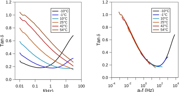
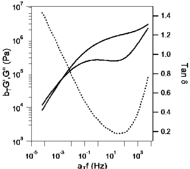
All these characteristic timescales can be experimentally determined using linear rheology. For some polymers, a general equivalence has been observed between the response to stress at low temperature and to that at high frequency (or short times). Similarly, an equivalence between the response at high temperature and that a low frequency (long times) is observed. This Time-temperature principle is true only in systems where the relaxation processes all vary with the same temperature-dependency. If so, it is possible to probe the mechanical response of a material at different temperatures and to draw a unique frequency-dependent master curve at a given temperature. This concept will be further detailed in the next chapter. Figure 12 plots, at 25°C, the

CHAPTER 1 - 2. Introduction to the adhesion of soft materials

16

storage and loss modulus G’ and G’’ as a function of reduced frequency and shows all the above-mentioned relaxation times of 1,4-polybutadiene [7].

Figure 12 Master curve represented at a reference temperature of 25°C for a 1,4-polybutadiene sample. Figure from Colby [7]

Prior to showing the relevance of polymer dynamics on their adhesion behavior, let us introduce the key concept underlying my thesis.

2 Introduction to the adhesion of soft materials

Two materials brought in contact interact, and Dupré proposed an expression for the thermodynamic work of adhesion in the case of ideal interface separation:

𝑊𝑎𝑑ℎ = 𝛾₁+ 𝛾₂− 𝛾₁₂ 1. 25

With γ1 and γ2 the surface energies of materials 1 and 2, and γ12 their interfacial energy.

Figure 13 Illustration of an ideal interface separation between two solids, and their corresponding surface energies

Yet if one considers two stiff materials (metal plates for example) and bring them into contact, hardly any energy is needed to debond them. On the opposite, adhesion properties of two very viscous materials (fluids for example) are also barely measurable. Why? In the first case, solids are rough surfaces, and if they are not able to deform, intimate contact between both surfaces is hardly achievable, hence weak macroscopic adhesion properties. On the other side, viscous materials are able to deform to create intimate contact but are not able to resist any mechanical loading due to their poor bulk properties. These examples show that for materials to exhibit high adhesion strength, they must be deformable enough to maximize contact area, and at the same time resistant enough to withstand high stresses. Therefore, viscoelastic soft materials are ideal for such applications and among them, the adhesive strength of Pressure Sensitive Adhesives (PSAs) and elastomers have been widely investigated.

17

2.1 Adhesive performance of soft materials

2.1.1 Pressure Sensitive Adhesives (PSA) as soft adhering materials

PSAs are soft materials that are able to adhere to any kind of surfaces through the application of light pressure. Their adhesion strength is due to very important number of physical interactions at the interface, without any chemical reaction or solvent evaporation, and to adequate rheological properties. Dahlquist [8] indeed proposed several criterias for PSAs to show optimum bonding properties. He suggested that the best application temperature is 50-70°C above the glass transition temperature of the material, and that the material must have a shear elastic modulus G’ at the bonding frequency lower than 0.1MPa for the layer to create intimate contact within the contact time. PSAs are highly deformable and are therefore able dissipate a high amount of energy during their debonding, thus exhibiting very high adhesion strength [9][10][11].

Figure 14 Image of a 90°-peeling test on a PSA.

In this thesis, another category of soft materials is studied: uncrosslinked elastomers. Yet whereas PSAs have modulus of the order of 0.1MPa, uncrosslinked elastomers are much more entangled and therefore much stiffer when tested at the 1s time scale; they exhibit moduli one order of magnitude higher than PSAs. This change in bulk properties is therefore expected to considerably change the contact formation. Moreover, PSAs are used on rigid surfaces, whereas this work is focused on the adhesion between two polymer melts. Therefore, even if the studies on PSAs are insightful for adhesion phenomenon, it is key to remember that the physics behind the bond formation and detachment of elastomers is expected to substantially differ.

2.1.2 Introduction to the tack behavior of elastomers

Tack is defined as the ability of two materials to resist separation after bringing them into contact for a short time under light pressure. If one considers two identical polymer melts in contact, that had had sufficient time to completely heal such that there are no interface, debonding leads to the measurement of the so-called green strength, which is the rubber’s mechanical resistance to deformation and fracture prior to vulcanization. Hamed has extensively studied the self-adhesion properties of uncured elastomers [12][13][14], and suggested that for rubbers to exhibit high tack, three main conditions needed to be fulfilled [15]. First, the two materials must come in intimate contact. If adsorbed gases are present (such as moisture or impurities), the effective molecular contact between the materials is reduced, preventing a sufficient flow of the polymer chains across the interface (see Figure 15).

CHAPTER 1 - 2. Introduction to the adhesion of soft materials

18 Figure 15 Illustration of adsorbed gases at the interface. Picture from Hamed [15]

Figure 16 Illustration of the interdiffusion of polymer chains across an interface

Furthermore, once contact between surfaces is achieved, polymeric chains are able to flow across the interface. This inter-diffusion enables healing of the interface, resulting in good adhesion properties [16][17]. Not only are good contact area and sufficient inter-diffusion of chains needed to reach good properties, but a high cohesive strength is also crucial. Indeed, during the debonding of a joint, both the interface and the bulk of the material are strained.

The extent of these three criteria for adhesion and self-adhesion of elastomer will be extensively detailed in this chapter, and used throughout the thesis.

2.2 Macroscopic characterization of adhesion

Several tests have been developed in order to characterize the adherence between two materials. The appropriate test for a specific application should be chosen with regard to the type of material tested, but also to the performances that one needs to evaluate.

During the “rolling ball test” (also called “marble test”), a steel ball is dropped from an angled surface to a plane surface with the tested material. For a given thickness and modulus, the material’s adhesive properties are inversely related to the marble’s distance on the surface. The experimental parameters of this test are hardly controllable, it is therefore challenging to deduce an effective energy of adhesion. Yet it is a simple way to compare several adhesives and is used in some industries. Another way of measuring adhesive properties is the loop tack test: a loop of adhesive is brought into contact with a substrate and then removed at a constant speed. The force needed to remove the loop is measured and the failure energy can be evaluated [18]. In the adhesive community, the most common test is the peel test [19][20][21]. The material and its stiff backing are adhered to the substrate and its extremities are clamped to a tensile machine. Different test geometries are possible, depending on the angle between the applied force and the substrate. The adhesion energy is computed by measuring the force necessary to keep a certain debonding speed. Contact times from tens of seconds to several minutes (and hours) are reached.

Rolling ball test Loop test Peel test

19

During this work, the adhesion properties are characterized with a probe tack device [10] which will be presented more in details in Chapter 3.

2.3 Comments

During this part, it was shown that adhesion of two elastomers depends on several material-related properties, and several methods have been presented to characterize them. The characterization of adhesive joints is a two-stage process: bond formation and bond rupture. The mechanisms related to the contact- or interface- formation can thus be analyzed separately from those related to the debonding process. Both must be finely controlled for elastomers to exhibit high tack strength. The following paragraph will first focus on the formation of a strong interface and section 4 then introduces the energy dissipation processes needed to develop high adhesion.

3 Formation of a strong interface

As mentioned previously, materials must create intimate contact on a molecular scale, and form interfacial interactions to exhibit high tack properties. Several theories have been proposed to explain the origin of these interactions and the development of adhesion between two surfaces on the molecular scale.

3.1 Molecular theories

Among the past hundred years, several theories have tried to explain the very complex phenomenon occurring at the interface between two contacting materials to explain their adhesion energy. Among those, the adsorption theory [22] considers adhesion as a purely surface process caused by intermolecular forces when the materials are close enough. These intermolecular forces include dispersion forces and hydrogen bonding. Nevertheless, this theory is unable to justify for several observed phenomenon: it cannot account for high adhesion energies between two nonpolar materials, and the adhesion energies expected from molecular forces are several magnitudes lower than that measured with peel tests. To account for these facts, the electric theory of adhesion was developed by Derjagin and Krotova [23], and suggest that adhesion is due to charges interactions at the surface. This theory cannot alone provide an explanation for polymer-to-polymer adhesion, and more specifically to polar polymers. Voyutskii and coworkers [16][24] developed the diffusion theory to explain adhesion in such systems. This theory states that the controlling mechanisms for adhesion between two polymer layers is the interdiffusion of polymer chains across the interface. Anand and coworkers [25] argue that polymer flow occurs only once intimate contact is occurred. In fact, in their contact theory, it is suggested that the main controlling mechanism for the adhesion between polymers is the contact stage.

Both the contact and diffusion theory are widely discussed in the literature, and their relevance regarding the self-adhesion of polymer melts are studied.

3.2 Formation of intimate contact

According to Anand and coworkers, self-adhesion (also called “autohesion”) consists of two main steps: a first one during which the contact between both surfaces is established, followed by a bond formation step i.e. development of interfacial forces. The first step, creation of intimate contact, is tackled during this section whereas the extent by which intermolecular forces (and especially interdiffusion) develop tack strength is dealt with in the next section (3.3).