Numerical simulation for coupling creep and damage of concrete on size effect plot

HAL Id: hal-01911030

https://hal.archives-ouvertes.fr/hal-01911030

Submitted on 2 Nov 2018

HAL is a multi-disciplinary open access archive for the deposit and dissemination of sci-entific research documents, whether they are pub-lished or not. The documents may come from teaching and research institutions in France or abroad, or from public or private research centers.

L’archive ouverte pluridisciplinaire HAL, est destinée au dépôt et à la diffusion de documents scientifiques de niveau recherche, publiés ou non, émanant des établissements d’enseignement et de recherche français ou étrangers, des laboratoires publics ou privés.

Numerical simulation for coupling creep and damage of

concrete on size effect plot

Rani Desiassyifayanty, Frédéric Dufour, Heru Purnomo

To cite this version:

Rani Desiassyifayanty, Frédéric Dufour, Heru Purnomo. Numerical simulation for coupling creep and damage of concrete on size effect plot. Journal of Contextual Economics-Schmollers Jahrbuch, 2004, 5 (2). �hal-01911030�

NUMERICAL SIMULATION FOR COUPLING CREEP AND DAMAGE

OF CONCRETE ON SIZE EFFECT PLOT

RANI DESIASSYIFAYANTY

University of Indonesia, Civil Engineering Department, Depok 16424, Indonesia E-mail : ra_lan@yahoo.com

FREDERIC DUFOUR

Research&Development, Genie Civil, Ecole Centrale de Nantes, 1, rue de la Noe, BP 92101, 44321 Nantes Cedex 3, France

HERU PURNOMO

University of Indonesia, Civil Engineering Department, Depok 16424, Indonesia

ABSTRACT

Numerical simulation for coupling creep and damage of concrete structures are presented in this paper associated with size effect law proposed by Bazant. Its behavior was investigated through two kinds of studies, the loading rate effect and residual capacity test. Three different sizes of beam, which is geometrically similar specimen, were simulated in three point bending test and creep test divided into load level test and residual capacity test. Numerical simulation was done using existing finite element code Aster_code developed by EDF (Electricite de France) for coupled between local damage based on bi-linear elasto damage model and creep based on Benboudjema’s theory. Result show that the finite element code is capable to reproduce the experimental result qualitatively. The interaction between creep and damage is shown through size effect plot by giving the behavior shift to the right, which means that the materials become more brittle when creep appears.

KEYWORDS

Concrete, Damage, Creep, Coupling, Size Effect, Load level 1. INTRODUCTION

Concrete has been used in structural construction for a long time and nowadays, its technology become more sophisticated. In the management of nuclear power plants that are often exposed to high stresses for a long time, the industrial problematic associated to the phenomenon of coupling creep - damage essentially focuses on the potential influence of the air pressure tests of the confinement surrounding wall, on the risk of concrete damage, and by way of consequences, of the increase of the leak rate.

The phenomenon of coupling creep-damage can be observed through two kinds of studies, the loading rate effect and residual capacity test. Gettu and Bazant (1992) have studied the loading rate effect and the scale effects on fracture growth. They found that the material becomes more brittle with decreasing rate of loading, the peak loads decrease, and the size of the fracture process zone for a crack propagation in mode I decreases too [1-2]. Rusch (1960) has

carried out experimental tests which results that the residual capacity of a structure subjected to creep solicitation prior to failure decreases when increasing the creep loading duration [3].

In common practice, it is usually assumed that linear visco-elasticity takes place for low load levels and that the instantaneous mechanical is elastic. On the other hand, for high load levels, cracks grow and interact with visco-elasticity [3-5]. Some experimental tests have been done in Ecole Centrale de Nantes for fracture and creep test. It shows that the mechanical response of a concrete beam changes when load applied to the beam after some duration of time. Under constant small or low load level, the creep grows and produces deformation with increasing time without any significant material damage and linear creep can be used. Nevertheless, when ultimate limit state analysis is performed to design concrete structural members, the state of stress can be moderately high and structures compromised by creep deformations for their long-term serviceability, resulting in a drastic reduction of their designed life span. Here, creep are associated also with micro-cracking nucleation and growth with time and consequently, to damage (Neville 1970; Proust and Pons 2001), which may result in concrete failure after a finite time interval (called failure by tertiary creep). Concrete exhibit a non-linear stress-strain response due to several mechanism [6-7]. In tension-dominated problems, micro-cracking occurs and results in a progressive degradation of the elastic properties of the material [3]. Experimental test concludes that there is a coupling between creep and damage.

This paper describes the numerical simulation using finite element computation

Aster_code developed by EDF to reproduce the experimental result qualitatively for coupling

creep and damage model calibrated from size effect tests on notched specimens. Local damage model is calibrated from size effect test in order to find the best fit to non local damage model and experimental result. Coupling creep and damage is investigated through two kinds of studies loading rate effect and residual capacity test in time variable.

2. DAMAGE MODEL

The failure of many materials such as concrete is due to the propagation and coalescence of microcracks. This phenomenon, which is called damage, is most often treated as strain softening in structural analysis. For the case of concrete, we know that concrete contains numerous microcracks even before the application of the external loads. These initial cracks, especially at the aggregate–cement paste interface, are caused among other things by segregation, shrinkage, or thermal expansion in the cement paste. Under the applied loading, the initiation of new microcracks and the growth of existing microcracks contributed to the nonlinear behavior in concrete.

Continuum damage mechanics is a framework for describing the variations of the elastic properties of a material due to micro-structural degradations. Its application to the quasi-static response of ductile and brittle materials came later on, mostly in the 80’s, but it was essentially limited to the prediction of the inception of cracking because the issues of ill-posedness due to softening and strain localization needed still to be tackled properly. It is with the development of non local (integral and gradient) damage models, that the theory found its widest range of applicability, covering within a single- still continuum based approach-crack inception and crack propagation in a format which could be conveniently implemented in general purpose finite element software [8-12].

2.1. Mazars Model

Its models based on local approach to describe the constitutive behavior by introducing a scalar variable d that quantifies the influence of microcracking [8-12]. This model also describes directly the slope of rigidity and the softening behavior. The stress-strain relation reads:

( )

0

σ = 1-ij d Eijkl kl (1)

where is the stress component, is the strain component, d is the damage variable and is the stiffness tensor of the undamaged material. The stress-strain relationship used by

Mazars (1984,1986):

σ

ij kl 0 ijkl E 0 0 0 0 1 σ (1 ) (1 ) ij ij kk ij v v E d E d + = − − − ⎡⎣σ ⎤⎦ (2)

According to this assumption, the Poisson’s ratio is not affected by damage.

However, for general states of stress, damage evolution should be related to some scalar quantity, function of the state of strain. For concrete, Mazars (1984) proposed called a positive equivalent strain as the intensity of local deformation:

%

(

)

2

i +

=

∑

% (3)

where εi are the principal strain and <εi >=εi when _i>0 otherwise < _i>=0 when _i=0.

In order to capture the differences of mechanical responses of the material in tension and compression, Mazars proposed to split the damage variable into two parts by linear relation defined as:

α

t t

α

c c

d

=

d

+

d

(4)

where dt and dc are the damage variables in tension and compression. They are combined with

the weighting coefficients αt and αc defined as function of the principal values of the strains

and due to positive and negative stresses. In uniaxial tension α

t ij c

ij t = 1 and αc =0. In uniaxial

compression αt = 0 and αc =1.

The evolution of damage is derived in an integrated form, as a function of the variable κ: 0 0 κ (1 ) 1 κ exp( (κ κ )) t t t t A A d B − = − − − 0 0 κ (1 ) 1 κ exp( (κ κ )) c c c c A A d B − = − − − (5) 0

κ , , , ,

A B A B

t t c c are the parameters in this model.

2.2. Bi-linear Elasto-Damage Model

The finite element code uses bi-linear elasto-damage model for damage modeling. The aim of bi-linear elasto-damage behavior is to model the possible simpler manner of elastic softening behavior. Its rigidity could decrease in an irreversible manner when the energy of strain becomes important, by distinguish the traction from the compression, to privilege the damage in

traction. The loss of rigidity measured by a scalar scaled from 0 (undamaged material) to 1 (material damage completely) [13].

The stress-strain relation is elastic, the rigidity is affected in a linear manner by the damage:

(

)

0

σ_ij = 1−d E_{ijkl kl} (6) Otherwise, the evolution of the damage, always increasing, is governed by the following function:

(

)

1

( )

, κ 2 f ε d = E − d where

( )

2 1 γ κ 1 γ y d w d + = + − ⎛ ⎞ ⎜ ⎝ ⎠⎟ (7)

The coefficient wy and γ, all two positives, are parameters of the model define the softening behavior. They are determined by a test of simple traction. The condition of coherency determines the rate of damage d& then completely:

( )

, 0

f d ≤ d&≥0 df&

( )

,d =0 (8) The Eq. (10) to (12) are sufficient to describe the law of bi-linear elasto-damage behavior entirely, in fact very simple. The Young modulus E and the Poisson ratio that determine the Hooke’s tensor by:

( )

1 1 σ σ σ E tr Id E E ν ν − ₌ + ₋ (9) To simplify the entry of the data of the model, one informs not wy and γ but directly the tangent module ET and the peak stress σy. Here are also the expressions of the strain to rupture εR in the simple traction test, as well as the volumetric energy k0 consumed to total damage of material point completely, this last expression being valid to either the history of loading:

1 1 σ R y T E E =

⎛

_⎜

−

⎞

_⎟

⎝

⎠

2 0 1 1 1 1 1 γ σ σ 2 2 γ y R y y T k w E E + =

⎛

_⎜

−

⎞

_⎟

= =

⎝

⎠

(10)

Figure 1: Simulation of simple traction test

2 σ 2 y y w E = (11) γ T E E = − (12) σ E E T < 0 εR σy ε

In the contrary case, the damage is gotten while solving f

( )

,d =0:

(

1 γ 1

)

y w d w = +

⎛

_⎜⎜

−

⎞

⎝

⎠

⎟⎟

where 1 2 w= E (13)

3. CREEP MODEL

Concrete continuously deforms in time under sustained load. This phenomenon is called creep. Creep is time dependent strain increase of a solid body under constant or controlled stress. Creep strain (at any time) can be divided into:

a). Basic creep

This phenomenon happens while the concrete is sealed or if there is no moisture exchange between the concrete and the ambient media. This present paper will be focused on it.

b). Drying creep

It is the additional creep experienced when the concrete is allowed to dry while under sustained load. It represent hygro-mechanical coupling between strain and water content changes [14].

In one term of creep test, after the stress load applies, the deformation pass through three stages of evolution shown in Figure 2 including:

¾ Primary creep during the strain rate decreases &

d

c

dt

⎛

₌

⎞

⎜

⎟

⎝

&

⎠

,

¾ Secondary creep corresponds to a constant rate , this rate decreases slowly in the time function for low load levels,

&

¾ Tertiary creep where increase rapidly leading to the ruined of the test. The strain that occurs in tertiary phase is connected to the loss of structure resistance due to the evolution of damage and the propagation of macrocrack in cement matrix [6].

& (t) t Primary creep Secondary creep Tertiary creep Undamaged material (ideal) tR

Figure 2: Schematic view of three phases of creep

The experimental analysis of the creep kinetics permits to put in evidence the existence of two different time scales in the behavior of the concrete under loading:

¾ Short-term creep, the basic creep kinetics strain is fast during some days after the loading. The short term creep is the diffusive mechanism of water in the capillary space leads by the application of a macroscopic loading (Wittmann 82): under macroscopic loading, the stress in the microscopic scale of the heterogeneous material are transmitted to shortcoming the assembly of the hydration products that surrounds the capillary pores.

¾ Long-term creep, the basic creep strain is characterized by a very slow kinetics. The mechanism to the origin of the long-term creep seems rather associates to a phenomenon in the nano-pores (it is said the pores of the hydrates) [Wittman 82]. The long-term creep resides in the shift of the C-S-H layers (Bazant et al. 97b)[6].

Benboudjema (2001) describes that basic creep is considered to be the result of two

processes, which are driven by the spherical and deviatoric component of the stress tensor, respectively. Several experimental findings prove that the splitting of the creep strain process to a spherical part and a deviatoric part is relevant (Glucklich et al. 1972, Gopalakrishnan et al. 1969,

Jordan et al. 1969, Benboudjema et al. 2001). Moreover, they showed that the spherical creep

strains and the deviatoric creep strains are proportional to the spherical part and the deviatoric part of the stress tensor [15-18].

Each part of the creep strain process is associated with a different chemo-physical mechanism. The decomposition of the basic creep strain vector εbc

reads below: 1

bc dev sph bc bc

= + (14)

where dev_bc and _bcsph are the spherical and the deviatoric creep strains. To take into account the effect of the internal humidity, the stress are multiplied by the internal relative humidity:

( )

σ

sph sph

bc =hf and

( )

σ

dev dev

bc

=

hf

(15)

where h states for the internal relative humidity.

3.1. Spherical Part

The spherical part is assumed to occur in the micro-porosity (0,01-50 µm range). It is associated to the migration of adsorbed water, located at the interface between hydrates and the hydrates intrinsic porosity, towards the capillary pores (Figure 3).

Its mechanism concerns water moving in both capillary space (reversible) and intrinsic porosity (irreversible), due to the hydrostatic component of the stress tensor.

Figure 3: Proposed mechanism for the spherical creep (Benboudjema et al. 2001)

ηsph r sph r sph r k ηsph i sph i sph i k

Figure 4: Phenomenological model associated with spherical part of basic creep

σ

_%

sph

σ

_%

sph

σ

_%

sph

σ

_%

sph Interfolliare water

By assuming that the behavior of the hydrated and the unhydrated cement particles are elastic and that the migration of water follows the Poiseuille equation, that adopted mechanism lead to the following system of equations:

1 σ 2 η i sph sph sph sph sph r r sph r h k =

⎡

_⎣

−

⎤

_⎦

− & % & (16)

(

)

1 σ η sph sph sph sph sph sph sph sph sph r r i i r r sph i k k k h k + =

⎡

_⎣

− +

⎤ ⎡

_⎦

−

_⎣

−

⎤

_⎦

& % (17) sph sph sph r i = + with 2 x x x + = + (18)

where sph_r and sph_i are the reversible and the irreversible spherical creep strains,

η

sph_r and

η

sph_i are the apparent viscosities of the water at two different scales of the material (macroscopic and microscopic level). These apparent quantities depend upon the water viscosity and the connected porosity geometry. Further,

k

_rsph and

k

_isph are the apparent stiffness associated to the precedent viscosities and related to the stiffness of the porous material and the skeleton.

σ

%

sph is the spherical effective stress. The rheological model of this part is shown in Figure 4.

3.2. Deviatoric Part

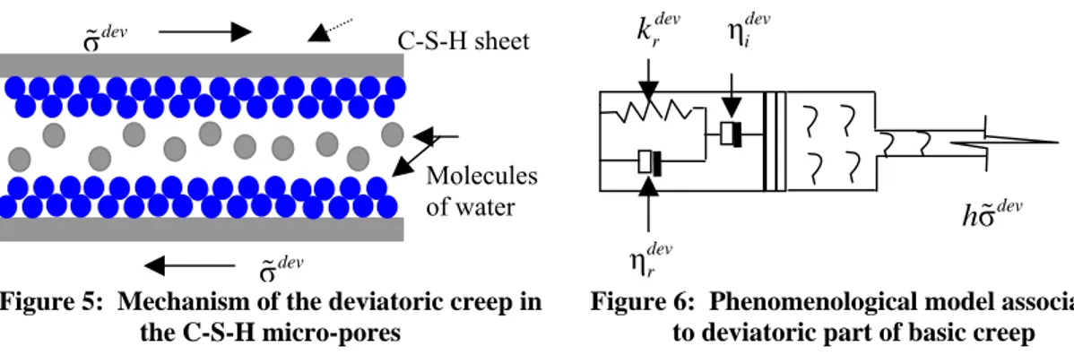
The deviatoric part is supposed to be caused by the sliding of the C-S-H layers (Benboudjema 2002). This phenomenon occurs in the nano-porosity (dimension of about 1 nm). The deviatoric creep mechanism is presented in Figure 5.

Figure 5: Mechanism of the deviatoric creep in the C-S-H micro-pores

k

_rdev

η

_idev

h %

σ

dev

η

dev_r

Figure 6: Phenomenological model associated to deviatoric part of basic creep

σ

_%

dev

σ

_%

dev

C-S-H sheet

Molecules of water

As the case of the spherical part, the deviatoric strain vector is split in a reversible part and an irreversible part :

dev bc dev r dev i

dev dev dev

bc

=

r

+

i (19)

The reversible part is associated to the interfoliar adsorbed water (great adsorption energy). The irreversible part is due to the rupture of the hydrogen bridge in the interlamellar adsorbed water.

The physical mechanism of the deviatoric creep leads to constitutive relations:

( )

ηdev dev dev dev σdev

r &r +kr r rev =h%ii (20)

η

dev dev

σ

dev

i

&

i

=

h

%

(21)

4. SIZE EFFECT LAW

Bazant assigns the size effect to a stable propagation of the cracks until it reaches the

maximal effort, combine to a redistribution of the stress and a laxity of the energy stored generated by the cracks. The fact that the size of the fracture process zone in the material is independent from the size of the structure provided it does not interfere with its boundaries. Hence, the response of geometrically similar specimen is not geometrically similar and there is a size effect. It is due to energy redistribution from the rest of the structure (whose size changes from one specimens to another) where elastic energy is stored, to the fracture process zone whose size is constant [1].

For geometrically similar notched specimen, Bazant propose a relation link to the nominal stress of rupture σN (calculate based on elastic fragile model) to the characteristic size D

(the height of the specimen) (Bazant 1983):

0 σ 1 / t N Bf D D ′ = + (22)

D0 is a characteristic size, ft’ is the tensile strength of material, and B is a geometry-related

parameter. The nominal stress σN is determined from the maximum force Fmax shown in

following formula: 2 3 σ 2 (0.85 ) N Fl b D = (23)

For a sufficiently large size, the scale of the material inhomogeneity, and thus the material length, should become unimportant. So the power scaling law should apply asymptotically for sufficiently large sizes. If there is a large crack at failure, the exponent of this asymptotic power law must be –1/2 (see the dashed asymptote in Figure 7). For very small structure sizes, the size effect should again asymptotically approach power law. Because, for such small sizes, a discrete crack cannot be discerned (as the entire specimen is occupied by the fracture process zone, the exponent of the power law should be 0, corresponding to the strength criterion (see the horizontal dashes in Figure 7). The difficulty is that most applications of quasi-brittle materials fall into the transitional range between these two asymptotes, for which the scaling law that bridges the two power laws may be expected to follow some transitional curve (Figure 7).

Figure 7: Transitional scaling of the nominal strength of quasi-brittle structure failing only after large fracture growth

1 Strength material Log(D/D0) Usually from structure Usually from experimental test 2 LEFM Log(σN/Bft) D=D0

In a log-log plot, strength of material criterion is represented by a horizontal curve and

LEFM (Linear Elastic Fracture Mechanics) criterion is depicted by a line with the slope –1/2

(asymptotic power law). The two lines cut each other at the abscissa D/D0=1. D0 and Bft’ are

obtained from a linear regression which provides also the fracture energy Gf [19]. 2 0 0 2 1 1 with , and σ t f k c aD c D Bf G a c E ′ = + = = = 1 a (24)

5. COUPLING CREEP AND DAMAGE

Total strain rate

&

tot is defined as the sum of different contributions

tot = el + d + v + irr

& & & & & (25)

where

&

el is elastic strain rate (appearing in the incremental relation),

_&

d _{is strain rate due to}

damage,

&

vis nonlinear creep strain rate and

&

irris irreversible instantaneous strain rate. The stress rate can be written as:

σ ( tot d v irr)

eff E

= & −& −& −&

& (26)

It can be easily verified that, for instantaneous loadings, vanished and Eq. (26) reduced to constitutive equation for damaged concrete:

v

&

σ ( tot d irr)

eff E

= & −& −&

& (27)

whereas for low-stress long-term loading (creep with no damage), Eq. (26) reduced to classical visco-elasticity

σ& =E_eff(&tot −&v) (28) The present model is based on the assumption that only a portion of the total creep strain contributes to the damage evolution with time. The motivation is that for low stress levels there is no significant variation of the elastic modulus means that no significant damage. Hence, the equivalent strain is replaced an effective strain which is the sum of the instantaneous strain plus a fraction of the creep strain, i.e:

(

)

3 ₂ , 1 ( ) el d( ) α ( )cr eff i i i t t ₊ = =

∑

+ t (29)

where the creep strain is

, σ (1 ) cr tot el d tot v d EC = − = − − (30) and the coefficient α is considered for simplicity independent of the loading level but such that there is a good correlation between the experimental and the numerical results.

6. NUMERICAL SIMULATION 6.1. Modelization of the model

This numerical tests consist of three part of modelization including: ¾ Fracture Test Simulation,

¾ Loading Rate Simulation, and

¾ Creep Test Simulation, which is divided into two parts: loading level and residual capacity test.

The test was applied followed the experimental test using three different size of notched beams shown in Figure 8 which is geometrically similar specimens define in Table 1.

The geometry model is using 2D (two dimensional) configuration in plane stress model. It is a usual implementation for beam problems with criterion σzz=0 and zz≠0 (the normal

stress in z direction is zero or negligible), which is in plane displacements, the stresses and strains can be taken as uniform through the thickness. The elements use quadrilateral (Q8) with 8

nodes of Gaussian points. Due to symmetry, only half section is modeled. The mesh can be seen in figure 9 and 10 for non local and local model.

Figure 8: Three point bend experiments on notched specimen Table 1: Size of Beams

Beam Type Height (D) Length (L) Span (l) Thickness (b) Notches Depth

(a0)

D100 10 cm 35 cm 30 cm 10 cm 1.5 cm

D200 20 cm 70 cm 60 cm 10 cm 3 cm

D400 40 cm 140 cm 120 cm 10 cm 6 cm

Because of the symmetrical reason, the beam is not implemented as a full beam. It can be modeled in half beam with some boundary condition. The displacement was controlled in horizontal direction on the lines element located at half length of the beam with the height equal to the height of the beam (D) reduces by the height of the notches (a0). The horizontal

displacement in that line was managed to be zero in order to have the same behavior with full beam.

The boundary condition for support system locates in the bottom left edge of the beam. The vertical displacement was controlled to be zero at that point as the implementation of simple connection (v = 0).

Figure 9: Non local mesh Figure 10: Local mesh

L l

ao

D b

The applied load follows the three points bending test acts vertically at the upper right edge of concrete. It was treated as displacement imposed for fracture test and loading rate simulation. Otherwise, for creep test, the loads is applied in constant force for loading level test and continued to displacement imposed for residual capacity test.

The result of this modelisation is consist of several variable define as:

¾ Force (N), named load, was gotten from applying displacement imposed in fracture test, loading rate simulation, and residual capacity test. It is measured at the upper right side of

concrete. The result of force multiplies by two because we just modeless half of the beam. It also multiplies by 0.1 (the beam’s thickness = 10 cm) because we calculate in 2D which is for plane stress means the thickness is taken for 1 meter, otherwise we need the result in 3D related with the beam thickness.

¾ Vertical displacement (m), named displacement, is measured at the half-height of the beam on the half-length and the ends of it in order not to include the effect of local deformations at the support and load points. The vertical displacement is calculated by subtracts both values. ¾ Horizontal displacement (m), named COD (Crack Opening Displacement), is measured at

the end of the notch. The result is multiplies by two because of the half-beam model.

¾ Time (days), named time, is the instantaneous time defines from the time step _{∆t at the range}

t to t+∆t. It exists in loading level test.

Aster_code has just developed the coupled between local damage and creep model.

Therefore, some calibrations are needed by comparing the result from local damage model to non-local damage model. The calibrations are provided from damage model include the calibration of model parameter and scaling of the mesh. The parameter and the mesh got from this calibration are used for all calculation. The calibration is observed from the peak load values and the size effect plots.

The damage model use bi-linear elasto-damage model needs several model parameters as the input value. Some parameters can be modified such as the tension strength ft’, compression strength fc’, and softening parameters ET. Other parameter as internal length in non-local model can also be modified. Theoretically, by increasing the internal length and tension strength will increase the peak load. In other way, by increasing the softening parameters will decrease the peak load. In this simulation, the parameter that is modified is the softening parameter for mesh scaling from non local to local model. Notes that this model has the boundary condition ET<E.

On this model, generally the parameter that is used taken from the experimental parameter with several calibration in order to have a quite similar peak load value compare to numerical simulation. It describes as:

E = 39000 MPa

ET = - 1800 MPa

fc’ = 40.2 (fixed parameter) MPa

ft’ = 1.8 MPa

υ = 0.28

for non local model, there is one parameter called internal length that is exist. In integral model, the value of internal length lc states for the size of Fracture Process Zone (FPZ) is defined as:

lc = 3*da = 3*0.025 = 0.075 m,

where da is the maximum size of aggregate.

The non-local damage model use the gradient model that is for internal length defines as variable

c. The value is taken as (Pablo, 2004):

(

)

2 2

_{3 *}

14

14

a c

d

l

c

=

=

c = 0.0004017864 m2

Other parameters exist in creep model. For mechanical parameter, several values such as Young’s modulus and Poisson ratio are equal to damage model. The different to damage model is creep basically is a time-dependent problem. Therefore, the variable mentioned before is associated to some range of time.

¾ Young’s modulus (E) = 39000 MPa, constant for some particular time describes the definition of elasticity

¾ Poisson ratio (υ) = 0.28, constant for some particular time because in damage the Poisson ratio is always constant

¾ Relative humidity (h), is assumed to be 1, means using 100 % of the relative humidity with a constant behavior.

The creep parameter is based on Benboudjema model. The values of the parameter below are actually given from experimental test. It is includes:

¾ sph r

k

(K_RS) = 6.0e+4 ¾

η

sph r (ETA_RS) = 5.95e+8 ¾ sph i

k

(K_IS) = 3.0e+4 ¾

η

sph i (ETA-IS) = 2.4 e+4 ¾

k

_rdev (K_RD) = 3.4e+4 ¾

η

dev_r (ETA_RD) = 4.08e+11 ¾

η

dev_i (ETA_ID) = 2.33e+12

6.2. Fracture Test Simulation

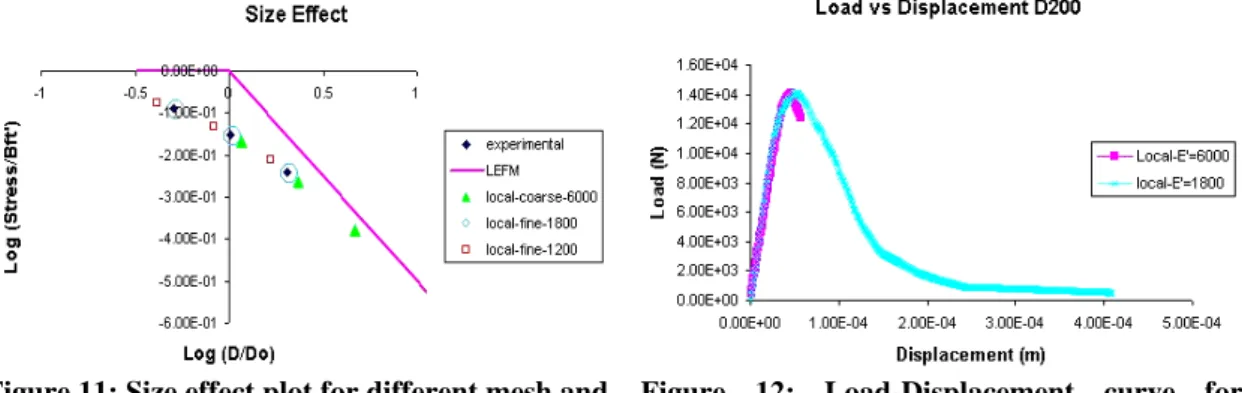
Fracture test simulation aims to find the average peak load for each size of beams. The simulation is performed follows three point bending test at a loading rate 0.1 mm/s until failure. Calibration for local damage model to non local damage and experimental result is done through size effect plot. Figure 11 shows the size effect plot of local model with different mesh discretisation and different softening parameter. We can see that by decreasing the softening parameter for the same mesh (local-fine-1800 and local-fine-1200), the plot gives behavior shift to the left. On the other word, the response of the beam becomes more ductile. Modifying the mesh and the softening parameter give the behavior shift to the left by decreasing the softening parameter and the mesh becomes finer. The response of the beam also becomes more ductile. Here, the shift distance is large.

Figure 11: Size effect plot for different mesh and softening parameter in local model

Figure 12: Load-Displacement curve for different mesh and softening parameter in local model

The behavior of pre-peak and post peak of the beam can be seen from Load-Displacement curves (Figure 12). The elastic part, which is the pre–peak behavior, is influenced by the Young’s Modulus E parameter and then softening ET parameter influences the post-peak behavior.

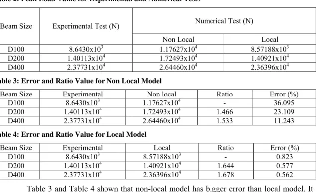
The comparison of peak load value between experimental and numerical in local and non-local model are presented in Table 2. We can see that the value of local model is closer to experimental test. The error values and the ratio for peak load in local and non local compare to experimental result are presented in Table 3 and Table 4.

Table 2: Peak Load Value for Experimental and Numerical Tests

Numerical Test (N)

Beam Size Experimental Test (N)

Non Local Local

D100 8.6430x103 1.17627x104 8.57188x103

D200 1.40113x104 1.72493x104 1.40921x104

D400 2.37731x104 2.64460x104 2.36396x104

Table 3: Error and Ratio Value for Non Local Model

Beam Size Experimental Non local Ratio Error (%)

D100 8.6430x103 1.17627x104 - 36.095

D200 1.40113x104 1.72493x104 1.466 23.109

D400 2.37731x104 2.64460x104 1.533 11.243

Table 4: Error and Ratio Value for Local Model

Beam Size Experimental Local Ratio Error (%)

D100 8.6430x103 8.57188x103 - 0.823

D200 1.40113x104 1.40921x104 1.644 0.577

D400 2.37731x104 2.36396x104 1.678 0.562

Table 3 and Table 4 shown that non-local model has bigger error than local model. It might be because in non-local model, we use the same softening parameter as in local model, although the mesh of both model are different. The difference of the mesh causes the difference of energy distribution in the model. Here, the softening parameter gives some influence to the peak load result.

Table 5: Ratio Value for Experimental Results

Beam Size Experimental Ratio

D100 8.6430x103 -

D200 1.40113x104 1.621

D400 2.37731x104 1.697

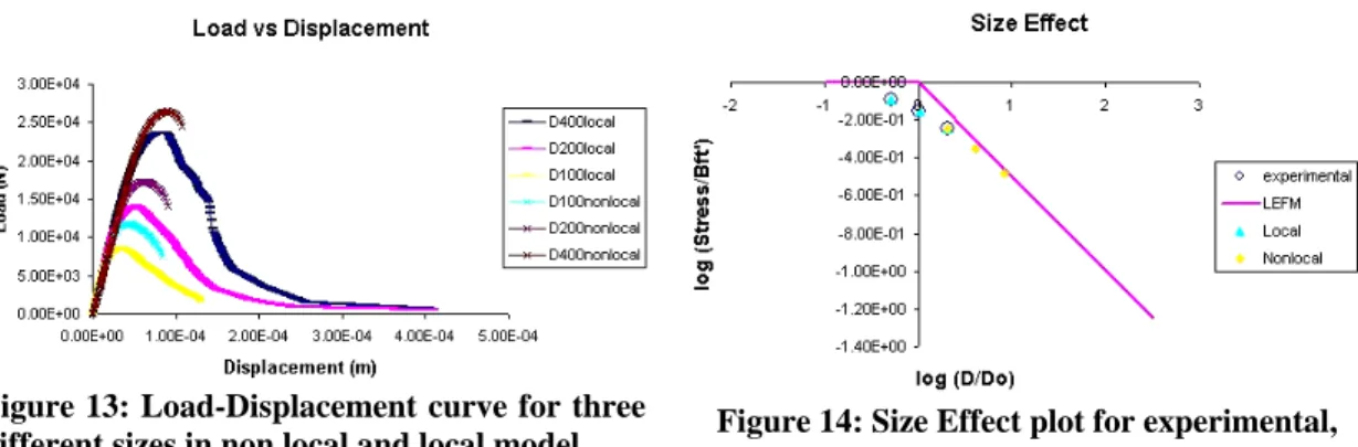
The difference between local and non-local can be seen from Load-Displacement curve (Figure 13). Generally, from Table 3-4, we can see that the ratio of the peak load for three sizes of beam in local and non local approximately similar in the range of 1.5-1.7. It is almost similar to the experimental result in Table 5.

Figure 13: Load-Displacement curve for three

different sizes in non local and local model Figure 14: Size Effect plot for experimental, _{non local and local model}

Size effect plot is one solution to calibrate the result of numerical to experimental test. Figure 14 shows that the local and non-local model plots around the experimental result. For the same model parameter, the non-local gives more brittle response than the local model. As mentioned before, it might be caused by the different mesh discretisation produces different energy of distribution.

The local model that is presented here will be used for the creep calculation, because the coupled model that exists is just between local damage and creep model.

6.3. Loading Rate Simulation

Loading rate effect simulates the behavior coupled creep and damage with different loading rate. The loading rate variable is implemented in time to peak variable, which is for this numerical simulation defines as:

¾ Second, time to peak is 1 second. The loading rate ∆ &uis 0.1 mm/s ¾ Minute, time to peak is 60 second. The loading rate∆ &uis 1.6667e-3 mm/s ¾ Hours, time to peak is 3600 second. The loading rate∆ &uis 2.7778e-4 mm/s ¾ Day, time to peak is 86400 second. The loading rate∆ &uis 1.1574e-6 mm/s ¾ Week, time to peak is 604800 second. The loading rate∆ &uis 1.6534e-7 mm/s ¾ Month, time to peak is 2592000 second. The loading rate∆ &uis 3.8580e-8 mm/s The time step for all time variables are keeping the same equal to∆t= 0.1 second.

The behavior of pre-peak and post-peak of the beam subjected to creep can be seen through Load-Displacement curve (Figure 15). It shows that for short time loading (second and minute), the sense of creep has not clearly propagated. The curve behavior is almost similar like the curve resulted from fracture test. Here, the behavior is still elastic.

Figure 15: Load-Displacement curve on medium

The behavior of long time loading (hour, day, week and month) is considered to become visco-elastic. The creep has appeared at this time associated to damage phenomena. From the curve we can see there is a little change in the peak load, which is decreasing by increasing the time to peak. Its behavior can be observed clearly in size effect plot.

The size effect on loading rate is shown in Figure 16. Increasing time to peak gives the behavior shift to the right in size effect plot. We can observe that the response of the beam become more brittle by decreasing the loading rate, with the consequences that the peak loads also decreases. Noted that for short term loading, as mentioned before, the shift from one second to one minute is too small, which can be assumed as the same, because of in this loading time, the creep has not propagate yet. The shifting starts to give a quite large distance from one hour. Quantitatively, this model is capable to produce the loading rate effect observed by Bazant.

6.4. Creep Tests Simulation

Several studies have been done related to the problem of coupling between creep and damage. Practically, it is usually assumed that linear visco-elasticity takes places for low load levels and that the instantaneous mechanical behavior is elastic. For high load levels, cracks grow and interact with visco-elasticity.

Experimental result for residual capacity of a structure subjected to creep solicitation prior to failure decreases when increasing the creep loading duration. Size effect plot give the behavior shift to the right by increasing the percentage of the peak load [6].

The modelisation of this test in numerical simulation can be illustrated as:

¾

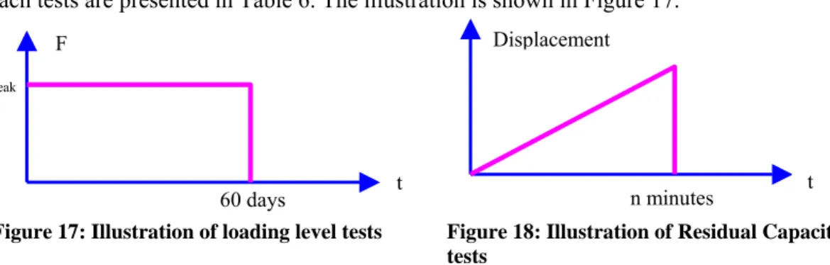
For the loading level test, the beam is applied by a constant load value implemented in the percentage of the peak load (50-80% of the peak load) for 60 days. In this test, the beam should be assured not to break. The peak load is measured from instant loading. The value of each tests are presented in Table 6. The illustration is shown in Figure 17.

Figure 17: Illustration of loading level tests Figure 18: Illustration of Residual Capacity tests n minutes Displacement t 60 days % Fpeak F t

¾ For the residual capacity test, three point bending test until failure is carried out on the beam immediately after loading level test. In the numerical simulation, the applied variable is in displacement form at the same loading rate. The illustration is shown in Figure 18.

Table 6: Applied load in Loading Level tests

Applied Load D100 D200 D400 50% Fpeak 4.28594x103 7.04605x103 1.18198x104 60% Fpeak 5.14313x103 8.45526x103 1.41838x104 70 % Fpeak 6.00032x103 9.86447x103 1.65477x104 75 % Fpeak 6.42891x103 1.05691x104 1.77297x104 80 % Fpeak 6.85750x103 1.12737x104 1.89117x104

6.4.1. Loading Level Test

It is expected that visco-elasticity and crack growth interaction related to the solicitation level. Thus, under high-sustained loads, damage occurs and the role of microcracking on creep evolution is exhibited. It has also been verified that, creep in compression is significantly affected by applied load amplitude. The greater the load level, the larger the creep strain magnitude.

The numerical simulation is done for three sizes of beam varied in different loading level (Figure 19). The curves indicate that by increasing the percentage of the peak load, in other word is increasing the load levels, the time to failure will decrease and the displacement increases. The displacement that is measured here is the total displacement consists of instantaneous displacement and creep displacement. Moreover, experimentally, creep develops very fast in the first days of loading and stabilizes after a few weeks for the lower load levels (50 % and 60 %). Concerning the specimen loaded at 80 % of peak load, the failure occurred 2.8 days after applying the load.

Other simulation is done for different size of beam with the same load level. Figure 20 shows for 70 % of peak load. Experimentally, at the same loading level, the beam will have more chance to break earlier in larger size. Apparently, in numerical simulation of 70 % from peak load, there is an exception in small size D100, which breaks after 24 days of applying load. There is possibilities that might become the reason of this condition. The reason might be because of numerical problem.

Figure 19: Displacement-Time curve on large beam at different loading level

Figure 20: Displacement-Time curve on different size of beam at 70 % of peak load 6.4.2. Residual Capacity Test

The interaction between creep and fracture of concrete is considered through the associated size effect in structures and the decrease of the fracture energy due to creep. In residual capacity test, after 60 days of loading, the beams subjected to 30 % and 40 % of peak load were removed from creep frames and then immediately subjected to three point bending loading up to failure with a constant loading rate. All specimens were kept under the same relative of humidity. Based on experimental result, for unotched beam, the maximum carrying force of the specimen subjected to creep initially is reduced of about 20 % in comparison with those of the unloaded specimen. Furthermore, it is found that there is no significant impact of the loading level on the response of the beam. For instance, on 50 % and 60 % loaded specimens have approximately the same peak load. Contrarily to previous result, on notched beam, there is no influence of the 60 days of basic creep loading on the residual capacity of bending beams. The peak load for loaded specimen and unloaded specimen is approximately the same.

The numerical simulation is done to produce the experimental test. Table 7 presents the peak load value for unloaded specimen (specimen without creep test) and loaded specimen (specimen with creep test) for 30 % and 40 % of the peak load. Generally, we can observe that for the same beam size, increasing the loading level will decrease the peak load. Furthermore, the peak load will decrease in loaded specimen compare to unloaded specimen. Here probably because the fracture energy decreases due to creep. In addition, we can see it from Load-Displacement curve on Figure 21.

Table 7: Peak Load value for loaded and unloaded specimen

Beam Size Unloaded specimen 30 % peak load 40 % peak load

D100 8.57188x103 8.17310x103 8.13512x103

D200 1.40921x104 1.35169x104 1.34645x104

D400 2.36396x104 2.19358x104 2.13938x104

Figure 21 shows the Load-Displacement curve on medium size for unloaded specimen compare to loaded specimen subjected to 30 %, 40 % and 50 % of the peak load. The same as experimental result, in numerical simulation there is no particular influence of 60 days of creep loading on the residual capacity of bending beams compare to the response obtained from unloaded specimen. Although there is a reducing in the peak load, it does not give a precious value means that the difference is so small. In the load-displacement plot for medium size, the decreasing can not be described clearly.

Figure 21: Load-Displacement curve on different load level of loaded specimen and unloaded specimen in the same beam size

Figure 22: Load-Displacement curve on different size of beam without creep and with creep at 30 % of loading

Figure 22 show the Load-Displacement curve on different size of beam for unloaded specimen and loaded specimen subjected to 30 % of peak load. We can see that for small and medium size, the curve for loaded and unloaded specimens give a little difference. Otherwise, on large size, the difference of loaded and unloaded specimen give a significant value. It might be because on large size, the creep and damage propagate very fast that causes the curve reaches the softening part earlier. Consequently, the peak load is decrease significantly compare to the specimen without creep test. The investigation of this condition is also presented in size effect plot.

Figure 23 presents the size effect plot for unloaded specimen compare to loaded specimen subjected to 30 % and 40 % of peak load. Based on experimental result, the size effect plot gives behavior shift to the right from unloaded to loaded specimen. Numerical simulation observed that in size effect plot, the response of beam gives shift to the right from unloaded to loaded specimen, the same as experimental result. We also observed that by increasing the loading level, the plot shifts to the right. The response of the beams becomes more brittle by

increasing the load level because of the decreasing of the fracture energy due to creep. Here, we can see that there is a coupling between creep and damage. For unloaded specimen, the fracture phenomenon is only damage without creep because there is no time variable. Otherwise for loaded specimen, damage associated with creep phenomenon contains time variable gives influence to the response of the beam become more brittle.

Figure 23: Size Effect plot between loaded at 40 % and 30 % of peak load and unloaded specimen 7. CONCLUSION

The following conclusion can be drawn from the numerical result that has been done: ¾ The model developed by EDF in Aster_Code is capable to reproduce the coupled model

between creep model and local damage model.

¾ The appropriate mesh type that is used in this simulation is quadrilateral (Q8).

¾ The result calibration for local model from non-local model is done through size effect plot. It result is compared to experimental test. The local model gives almost similar result to experimental.

¾ For geometrically similar specimens, the peak load is neither equal nor multiplied by two. Numerical simulation result the ratio between one to another specimen is in range of 1.5-1.7. ¾ Loading rate effect gives behavior shift to the right by decreasing the loading rate means also

increasing time to peak. Consequently, the peak load decreases and the beam response become more brittle in LEFM region.

¾ For the same load level on different size of specimen, the beam will break earlier on larger size. Furthermore, for different load level on the same size of specimen, the beam will break earlier at high load level.

¾ For high load level, the tertiary creep i.e. a visco-elastic response of the material coupled with an evolution of damage occurs in numerical simulation. Tertiary creep is observed for load levels above 60 % of maximum carrying capacity of the beam measured on initially unloaded specimens.

¾ Residual capacity test shows that for low creep levels (30 % and 40 % of peak load), basic creep does not influence the structural strength of the beam.

¾ Size effect plot on residual capacity test shows that the transition from unloaded specimen to loaded specimen gives shift to the right, also by increasing the load level. The response of the beam becomes more brittle.

8. ACKNOWLEDGEMENT

The research presented in this paper was performed at Genie Civil, Ecole Centrale de Nantes, France as a realization of joint cooperation between University of Indonesia, Indonesia and Ecole Centrale de Nantes, France on the Post Graduate Program in Civil Engineering University of Indonesia. I would like to express my great appreciation to DUO-FRANCE programme who facilitates this research.

9. REFERENCES

[1] Bazant, Z.P. (2002), Scaling of Structural Strength, Helmes Penton Ltd., London.

[2] Bazant, Z.P., Li, Y.N. (1997), “Cohesive Crack with Rate Dependent Opening and Viscoelasticity II: Numerical Algorithm Behavior and Size Effect”, Int. Journ. of

Fracture, 86(3), 267-288.

[3] Omar, M., Pijaudier-Cabot, G., Loukili, A. (2003), ”Numerical Models for Coupling Creep and Fracture of Concrete Structures”, Computational Modelling of Concrete

Structures, Bićanić et al. (eds), Swets & Zeitlinger, Lisse, 531-539.

[4] Mazzoti, C., Savoia, M. (2004), “Nonlinear Creep Damage Model for Concrete under Uniaxial Compression”, J. Engineering Mechanics. ASCE, 129, 1065-1075.

[5] Mazzoti, C., Savoia, M. (2001), “An Isotropic Damage Model for Nonlinear Creep Behavior of Concrete in Compression”, Fracture Mechanics of Concrete Structures, de Borst et al (eds), Swets & Zeitlinger, Lisse, 255-262.

[6] Omar, M. (2004), Deformations Differees du Beton :Etude Experimentale et Modelisation

Numerique de L’Interaction Fluage-Endommagement, These de Doctorat, Ecole Centrale

de Nantes.

[7] Omar, M., Haidar, K., Loukili, A., Pijaudier-Cabot, G. (2004), “Creep Load Influence on The Residual Capacity of Concrete Structure: Experimental Investigation”, paper of

R&DO, Institut de Recherche en Genie Civil et Mecanique, Ecole Centrale de Nantes.

[8] Pijaudier-Cabot, G., de Borst, R., Mazars, J.(2001), “Continous Damage Models for Fracture of Concrete”, Fracture Mechanics of Concrete Structures, de Borst et al (eds), Swets & Zeitlinger, Lisse, 471-482.

[9] Pijaudier-Cabot, G., Ludovic, J., Huerta, A., Dube, Jean-Francois (2001), Chapter

3:Continuum Damage Modeling in Geomechanics, Fracture Mechanics of Concrete

Structures, de Borst et al (eds), Swets & Zeitlinger, Lisse, 471-482.

[10] Pijaudier-Cabot, G., Jason, L. (2002), “Continuum Damage Modeling and Some Computational Issues”, Revue Francaise de Genie Civil, Numerical Modeling in Geomechanics 6, 991-1017.

[11] Pijaudier-Cabot, G. (2003), “Continuum Damage Modeling”, Computational Modelling of

Concrete Structures, Bićanić et al. (eds), Swets & Zeitlinger, Lisse, 531-539.

[12] Ludovic, J., Gharmavian, S., Pijaudier-Cabot, G., Huerta, A. (2001), “A Benchmark for The Validation of a Non Local Damage Model”, Revue Francaise de Genie Civil, 8(2-3), 303-328.

[13] Badel, P. (2005), Loi de Comportement ENDO_ISOT_BETON, Manuel de Reference: Code_Aster, R7.01.04-B, EDF, France.

[14] Bazant, Z.P. (1988), Mathematical Modeling of Creep and Shrinkage of Concrete, Wiley,

[15] Benboudjema, F. (2001), “A Basic Creep Model for Concrete Subjected to Multiaxial Loads”, Fracture Mechanics of Concrete Structures, de Borst et al (eds), Swets & Zeitlinger, Lisse, 161-168.

[16] Benboudjema, F. (2003), “An Unified Approach for The Modelling of Drying Shrinkage and Basic Creep of Concrete”, Euro-C Conference on Computational Modeling of

Concrete Structures, St Johann im Pongau (Autriche), Balkema.

[17] Benboudjema, F.,Meftah, F., Torrenti, J.M., Sellier, A., Heinfling, G.(2001), “A Basic Creep Model for Concrete Subjected to Multiaxial Loads”, In 4th International Conference on Fracture Mechanics of Concrete and Concrete Structures, Cachan, 28-31

Mai 2001: 161-168, Balkema.

[18] Le Pape, Y.( 2004), Relation de Comportement UMLV pour le fluage proper du beton, Manuel de Reference: Code_Aster, R7.01.06-A, EDF, France.

[19] Le Bellego, C., Dube, J .F., Pijaudier-Cabot, G., Gerard, B. (2003), “Calibration of Non Local Damage Model from Size Effect Tests”, Europ. Journ. of Mechanics A/ Solids, Elsevier, 22, 33-46.