Diffusion approximation and short‐path statistics at low to intermediate Knudsen numbers

(1)

HAL Id: hal-01662703

https://hal.archives-ouvertes.fr/hal-01662703

Submitted on 13 Sep 2018

HAL is a multi-disciplinary open access

archive for the deposit and dissemination of

sci-entific research documents, whether they are

pub-lished or not. The documents may come from

teaching and research institutions in France or

abroad, or from public or private research centers.

L’archive ouverte pluridisciplinaire HAL, est

destinée au dépôt et à la diffusion de documents

scientifiques de niveau recherche, publiés ou non,

émanant des établissements d’enseignement et de

recherche français ou étrangers, des laboratoires

publics ou privés.

Diffusion approximation and short-path statistics at low

to intermediate Knudsen numbers

Guillaume Terrée, Stéphane Blanco, Mouna El-Hafi, Richard Fournier, Julien

Yves Rolland

To cite this version:

Guillaume Terrée, Stéphane Blanco, Mouna El-Hafi, Richard Fournier, Julien Yves Rolland. Diffusion

approximation and short-path statistics at low to intermediate Knudsen numbers. EPL - Europhysics

Letters, European Physical Society/EDP Sciences/Società Italiana di Fisica/IOP Publishing, 2015,

110 (2), pp.20007. �10.1209/0295-5075/110/20007�. �hal-01662703�

(2)

Diﬀusion approximation and short-path statistics at low

to intermediate Knudsen numbers

Guillaume Terr´ee1_{, St´}_{ephane Blanco}2,3_{, Mouna El Hafi}1_{, Richard Fournier}2,3

and Julien Yves Rolland4

1 _{Universit´e de Toulouse; Centre RAPSODEE, UMR CNRS 5302, Mines Albi; Campus Jarlard}

F-81013 Albi Cedex 09, France

2 _{Universit´e de Toulouse, UPS, INPT; LAPLACE (Laboratoire Plasma et Conversion d’Energie)}

118 route de Narbonne, F-31062 Toulouse cedex 9, France

3 _{CNRS, LAPLACE - F-31062 Toulouse cedex 9, France}

4 _{LMB, UMR CNRS 6623, Universit´e de Franche-Comt´e - 16, route de Gray, 25030 Besan¸con Cedex, France}

Abstract– In the field of first-return statistics in bounded domains, short paths may be defined as those paths for which the diﬀusion approximation is inappropriate. However, general integral con-straints have been identified that make it possible to address such short-path statistics indirectly by application of the diﬀusion approximation to long paths in a simple associated first-passage problem. This approach is exact in the zero Knudsen limit (Blanco S. and Fournier R., Phys. Rev. Lett., 97 (2006) 230604). Its generalization to the low to intermediate Knudsen range is ad-dressed here theoretically and the corresponding predictions are compared to both one-dimension analytical solutions and three-dimension numerical experiments. Direct quantitative relations to the solution of the Schwarzschild-Milne problem are identified.

A simple invariance property of diﬀusion random walks was independently identified in [1] and [2]: for parti-cles incident on a system Ω, distributed uniformly and isotropically at its boundary, the average length ⟨L⟩ of the particle trajectories inside the system before the first exit is invariant when changing the characteristics of the random walk (exponentially distributed path lengths and micro-reversibly distributed scattering directions); highly or weakly scattering, and isotropic, forward or backward scattering particles lead to the same average trajectory length, that is therefore only dependent on the system ge-ometry. For three-dimension walks

⟨L⟩ =4V

S , (1)

where V is the volume of Ω and S the surface of its bound-ary ∂Ω. Numerous applications were reported in fields such as biology, colloid physics, turbid media and radiative transfer [3–13]. Theoretical extensions were also addressed by Benichou and co-workers [14], providing significant advances in our understanding of random search strate-gies [15–17] and contributing to the field of Brownian

motion in confined geometries [18–20] (see also [21] for a review). A very significant and recent step forward was also made in [22], where the property could be rigorously extended to the scattering of waves in resonant, chaotic or Anderson-localized structures. Major advances can also be expected from the numerous contributions of Mazzolo and co-workers that have closely considered the links be-tween the physics and mathematics literatures, in partic-ular with the introduction of this property in the field of integral geometry as a generalization of the Cauchy for-mula [23–27], and a reconciliation with the Feynman-Kac formalism [28–31]. Their researches, especially those ad-dressing the full length distribution [32], led to the iden-tification of the following second property [33]: for any function f of the trajectory length, with a defined limit f0

in zero,

⟨f (L)⟩ = f0+ ⟨L⟩⟨f′(R)⟩, (2)

where R is the random variable corresponding to trajec-tory lengths until the first exit for particles starting uni-formly and isotropically from within the volume, with the only constraint that limx→+∞pR(x)f (x) = 0, where pRis

(3)

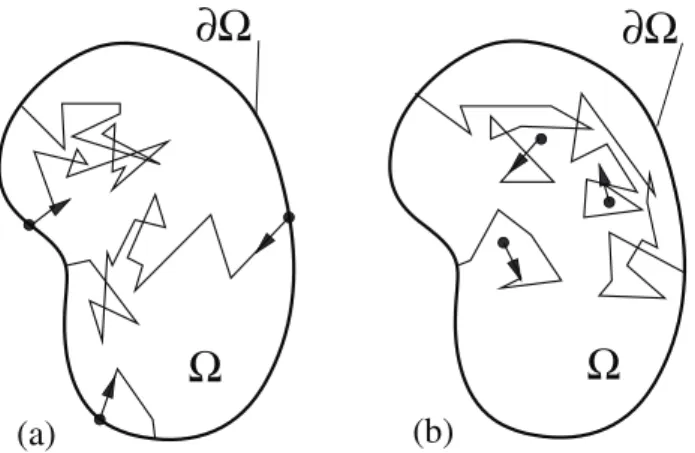
(a)

Ω

∂Ω

(b)

Fig. 1: Illustration of return L trajectories (a) and first-passage R trajectories (b).

the probability density function of R (see fig. 1(b)). The main interest of eq. (2) may be summarized the following way [33]: L trajectories start at the boundary and there-fore always include a non-negligible amount of short paths (particle returning to the boundary after a few scattering events, see fig. 1(a)) for which the diﬀusion approximation is inappropriate. In this sense, evaluating ⟨f (L)⟩ is a first-return problem. But ⟨f (L)⟩ can be exactly related to ⟨L⟩ and ⟨f′_{(R)⟩, where ⟨L⟩ is a known geometric quantity (see}

eq. (1)), and ⟨f′_{(R)⟩ is the solution of a first-passage}

prob-lem, which is easier to handle (in the present context) us-ing the diﬀusion approximation because the contribution of short paths decreases with the Knudsen number. We may therefore write ⟨f (L)⟩ in the zero Knudsen limit as

⟨f (L)⟩|Kn→0= f0+ ⟨L⟩⟨f′(Rdiﬀ)⟩, (3)

where Rdiﬀ is the random variable corresponding to the

diﬀusion approximation applied to R.

The particular case in which f (x) = xn_{, with n a strictly}

positive integer value, corresponds to the evaluation of the positive moments of L. The limit f0 is null and eq. (3)

becomes

⟨Ln_⟩|

Kn→0= ⟨L⟩n⟨R n−1

diﬀ ⟩. (4)

According to the properties of macroscopic diﬀusion, Rdiﬀ

scales as k = 1/λ∗_{, where λ}∗ _{is the transport mean free}

path (λ∗ _{reduces to the mean free path in the particular}

case of isotropic diﬀusion). This leads to

⟨Ln⟩|_Kn→0= αnkn−1, (5)

where αn is only dependent on the system geometry, and

not on the random walk characteristics. This result was pointed out in [33,34] as highlighting the contribution of short paths to ⟨Ln_{⟩: if only long L trajectories were to}

contribute to ⟨Ln_{⟩, the diﬀusion approximation could be}

directly applied on L and ⟨Ln_{⟩ would scale as k}n _instead

of kn−1_{. The authors then proposed a detailed physical}

picture for this quite counterintuitive reduction of the ex-ponent of k by 1 due to short-path statistics. Essentially,

large path-lengths scale indeed as kn _{but the probability}

to enter deep enough in the system scales as 1/k.

Coming back to the general case, eq. (3) is directly relevant to numerous application problems in which the numerical evaluation of first-return statistics in real geometries is either unfeasible or incompatible with com-putation time requirements. Such simulations use either stochastic methods of the Monte Carlo type, or deter-ministic methods based on phase-space discretisation of transport equations. Both approaches are known as com-putationally very demanding and the alternative consist-ing in the evaluation of ⟨f′_(R

diﬀ)⟩ using any standard

numerical solution of the macroscopic diffusion equation is obviously orders of magnitude faster, and is tractable whatever the geometrical complexity. One such practical example is optical diagnostic, in which numerical treat-ments are required for inversion of the measured signals, with real-time constraints (in particular in the pharma-ceutic and medical domains) which are such that solving the macroscopic diffusion equation is about the maximum affordable computational cost [35]. But what about all practical configurations in which intermediate Knudsen levels are encountered? We know that eq. (1) is rigorously valid independently of the Knudsen level: is there more behind this property that could be used for the evaluation of ⟨f (L)⟩ outside the zero Knudsen limit? In particular, can we obtain some theoretical benefits of the above-mentioned physical picture explaining why ⟨Ln_⟩|

Kn→0

scales as kn−1_{? These questions are addressed hereafter}

according to the following sequence: Available analytical solutions in the one-dimensional case are used to explore how eq. (5) is modified when increasing the Knudsen value. The observed features lead us to the proposition of an ap-proximate polynomial form of ⟨Ln_{⟩ in the general case.}

We then address the question of practically evaluating the polynomial coeﬃcients for complex three-dimensional ge-ometries, highlighting quantitative relations to the solu-tion of the Schwarzschild-Milne problem [36,37].

The characteristics of a diﬀusion random walk are en-tirely known given the mean free path λ(x) (the average of the exponentially distributed path lengths between suc-cessive scattering events) and the single scattering phase function p(us; ui, x) (the probability density function of

the scattering direction us for an incident direction ui).

Both are functions of the location x. When considering one-dimension walks (displacement along a line with in-stantaneous direction changes), the phase function can be chosen arbitrarily. Here we make the choice of isotropic scattering, which means that at each scattering event the probabilities to turn backward and to keep the same di-rection are both 1/2. In the particular case in which the mean free path is uniform and the considered system Ω is a segment of length a, the following analytical solution is available for ⟨Ln_{⟩ [33]:} ⟨(L/a)n⟩1D= n−1 ! i=0 βi,n 1 Kni (6)

(4)

Table 1: βi,n coefficients of the polynomial approximations of ⟨Ln⟩ (see eq. (7)), for the one-dimentionnal walk described in the text, as well as for three-dimensional walks in five geometries: a slab, a cube, a sphere, a spherical shell enclosed by two concentric spheres of radius R and 2R, and a volume composed of three identical cubes assembled according to a L shape (called tricube). For each geometry, a has been chosen equal to ⟨L⟩: ⟨L⟩ is indeed equal to the segment length in the one-dimensional case; and ⟨L⟩ is computed with eq. (1) for the three-dimensional geometries. The “line” coefficients are all analytical. For the five other configurations: β0,1 is obtained with eq. (1); βn−1,nare obtained as proposed in [33]; βn−2,n are computed with eq. (14); the other coefficients are evaluated, knowing βn−1,nand βn−2,n, using MC simulations. The MC simulations evaluate both ⟨Ln_{⟩ and ∂⟨L}n_{⟩/∂Kn between 1/Kn = 10 and 1/Kn = 50, and the displayed corresponding β}

i,ncoeﬃcients are the result of a Gauss-Markov linear fit (read [38]); for thus evaluated coeﬃcients, an estimation of the calculus error is given in square brackets. The number of sampled trajectories is about 109

.

Line Slab Sphere Spherical shell Cube Tricube

β0,1 1 1 1 1 1 1 β1,2 1/6 0.125 0.225 0.1394 0.2724 0.2531 β0,2 1 1.066 1.066 1.115 1.288 1.295 β2,3 1/20 28.13e-3 0.1085 35.80e-3 0.1707 0.1433 β1,3 1/2 0.3996 0.7193 0.4751 1.131 1.068 β0,3 1 1.828 [0.009] 1.235 [0.007] 2.050 [0.007] 2.187 [0.003] 2.357 [0.005]

β3,4 17/840 8.538e-3 73.23e-3 12.46e-3 0.1526 0.1155

β2,4 17/60 0.1698 0.6243 0.2314 1.300 1.132

β1,4 11/10 1.292 [0.004] 1.764 [0.005] 1.626 [0.006] 3.959 [0.008] 3.992 [0.007]

β0,4 1 4.564 [0.075] 1.794 [0.022] 5.857 [0.081] 3.214 [0.027] 4.214 [0.028]

with Kn = λ/a. The constants βi,n are given in table 1

(in the “Line” column) up to n = 4. The n-th mo-ment of L is therefore a polynomial function of degree n − 1 of the inverse of the Knudsen number. At the zero Knudsen limit, only the monome of higher degree remains and ⟨(L/a)n⟩1D|_Kn→0= βn−1,n/Knn−1, which is

compatible with the theoretical predictions of [33], with αn= βn−1,na2n−1 (see eq. (5)).

With this simple academic example, we can explore the accuracy level corresponding to the straightforward ap-plication of eq. (5) outside the zero Knudsen limit. The conclusions are that the 1% accuracy level is only reached beyond 1/Kn = 590 for ⟨L2_{⟩, 1/Kn = 980 for ⟨L}3_{⟩ and}

1/Kn = 1390 for ⟨L4_{⟩. Even a 10% accuracy level requires}

that the Knudsen number remains below 1/Kn = 50 (see the first line of table 2). Other calculations made on three-dimensional geometries lead to similar conclusions (see “monome” in table 2). This strongly restrains the range of the possible practical use of the theoretical derivations of [33], in particular for medical applications where the ac-curacy requirements are high and the Knudsen numbers always greater than 10−2_.

But the fact that the exact solution of the 1D problem has a polynomial shape over the whole Knudsen range gives us a simple indication concerning a possible exten-sion of eq. (5) to the intermediate Knudsen range for any dimension and any geometry. Outside the one-dimensional case, eq. (6) can indeed be seen as a polynomial approxi-mation of ⟨Ln_{⟩ in the limit Kn → 0:}

⟨(L/a)n⟩ = n−1 ! i=0 βi,n 1 Kni + O(Kn) (7)

with Kn = 1/(ka) and a any length scale characteristic of the considered system geometry. The meaning of such

a polynomial approximation is directly related to the fact that eq. (5) leads to limKn→0Knn−1⟨(L/a)n⟩ = αn

a2n−1 and the coeﬃcients βi,nare the n first coeﬃcients of the Taylor

expansion of Knn−1⟨(L/a)n⟩ with respect to Kn around Kn = 0. We held numerical experiments to explore the validity of eq. (7) in the low to intermediate Knudsen range. The coeﬃcients βi,n, obtained by model fitting of

Monte Carlo simulations, are given in table 1. The relative accuracies of resulting ⟨Ln_{⟩ predictions are better when}

decreasing the Knudsen range, as was observed with the monomial model of [33], but they are now of a few percent, or below one percent, in the Knudsen range typical of the above-listed applications (see the lines “polynome” in table 2).

For this modeling approach to become fully practical, the remaining question is: how to make the βi,n

coeffi-cients easily accessible to those who want to estimate the moments of L in any new geometry? A first solution is to perform Monte Carlo simulations, fit them with eq. (7), and mount tables of βi,ncoefficients for different geometry

classes. Such computations are very demanding, but they are to be done only once, as the βi,n are purely geometric

quantities.

We also started to think of pure theoretical alternatives. In [33], an exact expression was provided for the first coef-ficient (βn−1,n) as the solution of a macroscopic diﬀusion

process. The idea was that ⟨Ln_{⟩ = ⟨L⟩ n ⟨R}n−1_{⟩ could}

be expressed in an integral manner using the first-passage time probability density function (that of the R config-uration, i.e. when particles start uniformly within the volume), and that this density was the solution of a macro-scopic diﬀusion problem with null density at the boundary. Using a Hilbertian approach (expanding the distribution function), it can be shown that this solution corresponds

(5)

Table 2: Lower bound values of 1/Kn which with a 1% or 10% accuracy can be reached using the monomial [33], binomial, and polynomial approximations. The “line”, “slab”, “sphere”, “spherical shell”, “cube”, and “tricube” configurations are described in the caption of table 1.

Precision 1% 10% Moment ⟨L2_⟩ _⟨L3_⟩ _⟨L4_⟩ _⟨L2_⟩ _⟨L3_⟩ _⟨L4_⟩ line, monome 594 988 1390 54 88.0 130 line, binome 0 39.8 66.2 0 9.32 15.6 line, polynome 0 0 0 0 0 0 slab, monome 840 1400 2000 77 130 190 slab, binome 24 74 110 4.1 19 30 slab, polynome 24 16 12 4.1 4.3 4.1 sphere, monome 470 660 850 43 61 79 sphere, binome 3.4 31 45 0 7.5 12 sphere, polynome 3.4 3.9 1.2 0 0 0 spherical shell, monome 790 1300 1800 72 120 170 spherical shell, binome 22 69 110 0 17 28 spherical shell, polynome 22 12 6.3 0 0.69 2.9 cube, monome 470 660 850 43 62 80 cube, binome 6.7 32 47 0 7.9 12 cube, polynome 6.7 2.9 0 0 0 0 tricube, monome 510 740 970 46 69 92 tricube, binome 8.4 37 54 0 8.9 14 tricube, polynome 8.4 2.5 0.62 0 0 0

to a first-order approximation in Knudsen number. But the same Hilbertian reasoning establishes that the approx-imation becomes accurate to second order when using the Milne boundary condition [39]. This implies that both βn−1,n and βn−2,n can be deduced from the diﬀusion

ap-proximation as an n⟨L⟩βn−1,n= lim_Kn→0"Kn n−1 ⟨Rn−1⟩# = lim Kn→0"Kn n−1 ⟨Rdiﬀn−1⟩#, (8) an n⟨L⟩βn−2,n = lim_Kn→0 ∂ ∂Kn"Kn n−1_⟨Rn−1_⟩# = lim Kn→0 ∂ ∂Kn"Kn n−1_⟨Rn−1 diﬀ ⟩#, (9)

where Knn−1⟨Rn−1diﬀ ⟩ reads

Knn−1⟨Rn−1diﬀ ⟩ = $q a %n−1& +∞ 0 pdiﬀ(τ )τn−1dτ, (10)

with q the problem dimension and pdiﬀ the

probabil-ity densprobabil-ity of the dimensionless first-passage time at the macroscopic diﬀusion limit, using Milne boundary conditions. This density writes

pdiﬀ(τ ) = & ∂Ω u· ∇ρ(x; τ, Kn)dx, (11) ∂τρ(x; τ, Kn) = ∇2ρ(x; τ, Kn), ∀(x; τ ) ∈ Ω×[0; +∞[, ρ(x; τ, Kn) = ΛaKn u · ∇ρ(x; τ, Kn), ∀(x; τ ) ∈ ∂Ω×]0; +∞[, ρ(x; 0, Kn) = 1/V, ∀x ∈ Ω, (12)

where u is the inward normal unit vector at the bound-ary and Λ the extrapolation length. Λ = 1 in the one-dimentional case, and Λ ≃ 0.710446 in three dimensions with isotropic scattering [40]. Consequently, βn−1,n and

βn−2,n are directly related to the solutions, at Kn = 0, of

both the diﬀusion problem of eq. (12) and its associated derived one in s = 1

Λa ∂ρ

∂Kn. This leads to the following

coupled macroscopic diﬀusion problem: ⎧ ⎪ ⎪ ⎪ ⎪ ⎪ ⎪ ⎨ ⎪ ⎪ ⎪ ⎪ ⎪ ⎪ ⎩ ∂τρ(x; τ, 0) = ∇2ρ(x; τ, 0), ∂τs(x; τ, 0) = ∇2s(x; τ, 0), ∀(x; τ ) ∈ Ω × [0; +∞[, ρ(x; τ, 0) = 0, s(x; τ, 0) = u · ∇ρ(x; τ, 0), ∀(x; τ ) ∈ ∂Ω×]0; +∞[, ρ(x; 0, 0) = 1/V, s(x; 0, 0) = 0, ∀x ∈ Ω, (13) the solution of which allows to address βn−1,n as in [33]

and βn−2,n as βn−2,n = Λ⟨L⟩ n q n−1 a2n−2 & +∞ 0 pdiﬀ,s(τ )τn−1dτ, pdiﬀ,s(τ ) = +_∂Ωu· ∇s(x; τ, 0) · dx. (14)

These expressions are exact, which explains why βn−1,n

and βn−2,nhave no associated uncertainty values in table 1

where they are provided for a slab, a sphere, a cube, a tricube, and a spherical shell. Monte Carlo simulations were only used for βi,n with i ! n − 3. In practice, if

Monte Carlo simulations cannot be afforded, then these last coefficients can be neglected as a first modeling ap-proach. The binomial results of table 2 illustrate that this is sufficient to extend by one order of magnitude the range of Knudsen numbers addressed in [33].

(6)

REFERENCES

[1] Bardsley J. N. and Dubi A., SIAM J. Appl. Math., 40 (1981) 71.

[2] Blanco S. and Fournier R., Europhys. Lett., 61 (2003) 168.

[3] Eymet V., Fournier R., Dufresne J.-L., Lebonnois S., Hourdin F.and Bullock M. A., J. Geophys. Res., 114(2009) E11008.

[4] Anikeenko A. V., Medvedev N. N., Kovalev M. K. and Melgunov M. S., J. Geophys. Res., 50 (2009) 403. [5] Levitz P., J. Phys.: Condens. Matter, 17 (2005) S4059. [6] Challet M., Fourcassie V., Blanco S., Fournier R., Theraulaz G. and Jost C., Naturwissenschaften, 92_{(2005) 367.}

[7] Eymet V., Fournier R., Blanco S. and Dufresne J.-L., J. Quant. Spectrosc. Radiat. Transfer, 91 (2005) 27.

[8] Jeanson R., Blanco S., Fournier R., Deneubourg J.-L., Fourcassi´e V. and Theraulaz G., J. Theor. Biol., 225 (2003) 443.

[9] Benichou O., Loverdo C., Moreau M. and Voituriez R., J. Chem. Soc., 10 (2008) 7059.

[10] Condamin S., Tejedor V., Voituriez R., Benichou O.and Klafter J., Proc. Natl. Acad. Sci. U.S.A., 105 (2008) 5675.

[11] Vitkin E., Turzhitsky V., Qui L., Guo L. Y., Itzkan I., Hanlon E. B.and Perelman L. T., Nature (London), 2 (2011) 587.

[12] Weitz S., Blanco S., Fournier R., Gautrais J., Jost C. and Theraulaz G., Phys. Rev. E, 89 (2014) 52715.

[13] Zoia A., Dumonteil E. and Mazzolo A., Phys. Rev. E, 84 (2011) 61130.

[14] B´enichou O., Coppey M., Moreau M., Suet P. H. and Voituriez R., Europhys. Lett., 70 (2005) 42. [15] Tejedor V., Voituriez R. and Benichou O., Phys.

Rev. Lett., 108 (2012) 88103.

[16] Benichou O., Loverdo C., Moreau M. and Voituriez R., Rev. Mod. Phys., 83 (2011) 81.

[17] B´enichou O., Loverdo C., Moreau M.and Voituriez R., J. Phys.: Condens. Matter, 19 (2007) 065141.

[18] Condamin S., B´enichou O. and Moreau M., Phys. Rev. E, 75 (2007) 021111.

[19] Grebenkov D. S., Phys. Rev. E, 76 (2007) 41139. [20] Chevalier C., B´enichou O., Meyer B.and Voituriez

R., J. Phys. A, 44 (2011) 025002.

[21] B´enichou O.and Voituriez R., Phys. Rep., 539 (2014) 225.

[22] Pierrat R., Ambichl P., Gigan S., Haber A., Carminati R. and Rotter S., Proc. Natl. Acad. Sci. U.S.A., 111 (2014) 17765.

[23] Mazzolo A., Roesslinger B. and Gille W., J. Math. Phys. (N.Y.), 44 (2003) 6195.

[24] Mazzolo A., J. Phys. A, 37 (2004) 7095.

[25] Mazzolo A., Mulatier C. and Zoia A., J. Math. Phys., 55(2014) 83308.

[26] Mazzolo A., J. Phys. A, 42 (2009) 105002. [27] Mazzolo A., Ann. Nucl. Sci. Eng., 35 (2008) 503. [28] Zoia A., Dumonteil E. and Mazzolo A., EPL, 100

(2012) 40002.

[31] Zoia A., Dumonteil E. and Mazzolo A., Phys. Rev. Lett., 106 (2011) 220602.

[32] Mazzolo A., Europhys. Lett., 68 (2004) 350.

[33] Blanco S. and Fournier R., Phys. Rev. Lett., 97 (2006) 230604.

[34] Rolland J., PhD Thesis (Toulouse) 2009.

[35] Jacques L. and Pogue B. W., J. Biomed. Opt., 13 (2008) 041302.

[36] Chandrasekhar S., Radiative Transfer (Dover Publica-tions) 1960.

[37] Ishimaru A., Wave Propagation and Scattering in Random Media (IEEE Press) 1977.

[38] Orlande H. R. B., Fudym O., Maillet D. and Cotta R. M., Thermal Measurements and Inverse Techniques (CRC Press) 2011.

[39] Degond P. and Mas-Gallic S., Transp. Theor. Stat. Phys., 16 (1987) 589.

[40] Weinberg A. M. and Wigner E. P., The Physical Theory of Neutron Chain Reactors (Chigago Press) 1958.