AUTOMATIC MESH-BASED SEGMENTATION OF MULTIPLE ORGANS IN MR IMAGES
MAJID REZA MOHEB POUR
DÉPARTEMENT DE GÉNIE INFORMATIQUE ET GÉNIE LOGICIEL ÉCOLE POLYTECHNIQUE DE MONTRÉAL
THÈSE PRÉSENTÉE EN VUE DE L’OBTENTION DU DIPLÔME DE PHILOSOPHIAE DOCTOR
(GÉNIE INFORMATIQUE) AOÛT 2018
ÉCOLE POLYTECHNIQUE DE MONTRÉAL
Cette thèse intitulée :
AUTOMATIC MESH-BASED SEGMENTATION OF MULTIPLE ORGANS IN MR IMAGES
présentée par : MOHEB POUR Majid Reza
en vue de l’obtention du diplôme de : Philosophiae Doctor a été dûment acceptée par le jury d’examen constitué de :
M. BILODEAU Guillaume-Alexandre, Ph. D., président
M. GUIBAULT Francois, Ph. D., membre et directeur de recherche Mme CHERIET Farida, Ph. D., membre et codirectrice de recherche M. CAMARERO Ricardo, Ph. D., membre
DEDICATION
In memory of my mother To my family & dear wife With love and eternal appreciation
ACKNOWLEDGEMENTS
This thesis has been made possible through the help and support from many encounters. Notably, I am deeply thankful to all members of my Ph.D. committee who took patience to read and evaluate this manuscript. I am, of course, extremely grateful to my director, Francois Guibault, for his excellent guidance, support, caring, and patience during my Ph.D. study. I have learnt a lot from the sympathetic and supportive ambience of your personality. Also, I would like to express my great appreciation to my co-director, Farida Cheriet, for her supervision, help, valuable advice and corrections.
I would specially like to thank Dr. Julien Dompierre for his help and many insightful discussions and suggestions. This work could not have been succeeded without your help.
I take this opportunity to extend my sincerest thanks to all of my friends and colleagues at Polytechnique de Montréal for their valuable technical and emotional supports during all these years.
On a personal note, I must thank my close and deep friends, who gave me the courage to pursue the Ph.D. when times were darker, Amir Banani, Daneshmand’s family for their amazing kindness.
The most important of all in the world I thank my family; my late mother, Simin, who all my efforts in life are because of her love and happiness, my father, Ali, my sisters, Mitra & Samira and my brothers, Saeed & Vahid. Whatever I have in my life is because of your love and support. Your prayer for me was what sustained me thus far.
The best thing that happened to me during my journey at Polytechnique was to get to know my beloved wife, Azadeh, who enlighten my life with her presence. I thank you for being so understanding and for putting up with me through the toughest moments of my life. Your presence, love and support during these years of my study gave me lots of motivation to continue.
R
ÉSUMÉ
La segmentation de structures anatomiques multiples dans des images de résonance magnétique (RM) est souvent requise dans des applications de génie biomédical telles que la simulation numérique, la chirurgie guidée par l’image, la planification de traitements, etc. De plus, il y a un besoin croissant pour une segmentation automatique d’organes multiples et de structures complexes à partir de cette modalité d’imagerie. Il existe plusieurs techniques de segmentation multi-objets qui ont été appliquées avec succès sur des images de tomographie axiale à rayons-X (CT). Cependant, dans le cas des images RM cette tâche est plus difficile en raison de l’inhomogénéité des intensités dans ces images et de la variabilité dans l’apparence des structures anatomiques. Par conséquent, l’état de l’art sur la segmentation multi-objets sur des images RM est beaucoup plus faible que celui sur les images CT.
Parmi les travaux qui portent sur la segmentation d’images RM, les approches basées sur la segmentation de régions sont sensibles au bruit et la non uniformité de l’intensité dans les images. Les approches basées sur les contours ont de la difficulté à regrouper les informations sur les contours de sorte à produire un contour fermé cohérent. Les techniques basées sur les atlas peuvent avoir des problèmes en présence de structures complexes avec une grande variabilité anatomique. Les modèles déformables représentent une des méthodes les plus populaire pour la détection automatique de différents organes dans les images RM. Cependant, ces modèles souffrent encore d’une limitation importante qui est leur sensibilité à la position initiale et la forme du modèle. Une initialisation inappropriée peut conduire à un échec dans l’extraction des frontières des objets. D’un autre côté, le but ultime d’une segmentation automatique multi-objets dans les images RM est de produire un modèle qui peut aider à extraire les caractéristiques structurelles d’organes distincts dans les images. Les méthodes d’initialisation automatique actuelles qui utilisent différents descripteurs ne réussissent pas complètement l’extraction d’objets multiples dans les images RM. Nous avons besoin d’exploiter une information plus riche qui se trouve dans les contours des organes. Dans ce contexte les maillages adaptatifs anisotropiques semblent être une solution potentielle au problème soulevé. Les maillages adaptatifs anisotropiques construits à partir des images RM contiennent de l’information à un plus haut niveau d’abstraction représentant les éléments, d’une orientation et d’une forme donnée, qui constituent les différents organes dans l’image. Les méthodes existantes pour la
construction de maillages adaptatifs sont basées sur les intensités dans l’image et possèdent une limitation pratique qui est l’alignement inadéquat des éléments du maillage en présence de contours inclinés dans l’image. Par conséquent, nous avons aussi besoin d’améliorer le processus d’adaptation de maillage pour produire une meilleure représentation de l’image basée sur un maillage.
Dans le cadre de ce projet de doctorat, pour pallier au problèmes soulevés nous allons présenter une nouvelle méthode pour la segmentation automatique d’organes multiples dans les images RM en incorporant une technique d’adaptation de maillages. Dans une première étape, nous améliorons le processus d’adaptation anisotropique pour des maillages construits à partir d’images RM. Ainsi, les éléments du maillage sont alignés adéquatement avec le contenu de l’image et améliore l’anisotropie du maillage le long des contours dans toutes les directions. Ensuite, le maillage résultant est utilisé pour l’initialisation de modèles actifs multiples qui permettent d’extraire simultanément les frontières initiales des objets qui sont proches des frontières réelles d’organes multiples. Finalement, une méthode de convolution par champ de vecteurs est utilisée pour guider l’évolution de la courbe vers les frontières des organes afin d’obtenir les résultats de la segmentation finale avec une meilleure performance en termes de vitesse et de précision.
Plusieurs expériences et comparaisons ont été effectuées afin d’évaluer les différentes étapes de la méthodologie proposée. Notre méthode a été appliquée sur des séries d’images RM et les résultats obtenus démontrent sa capacité pour l’extraction simultanée de frontières approximatives initiales qui sont proches des frontières réelles d’organes multiples. Une comparaison a été effectuée entre la méthode proposée et trois autres méthodes distinctes pour l’initialisation automatique afin d’évaluer l’efficacité de la nouvelle approche d’initialisation et son impact sur la performance de la segmentation. La comparaison porte sur le nombre de modèles, le nombre d’itérations et le temps de convergence. Les résultats démontrent une amélioration de la convergence et de la vitesse des modèles actifs dans la segmentation d’organes multiples par rapport aux trois méthodes considérées. Afin d’évaluer la précision des résultats de segmentation, nous avons aussi effectué une comparaison entre les contours segmentés automatiquement à l’aide de la méthode proposée et ceux segmentés par un expert sur des images RM de colonnes vertébrales.
Cependant, la méthode proposée possède certaines limitations comme par exemple son échec dans l’extraction de descripteurs anisotropiques dans des régions à faible contraste et le fait qu’elle soit validée uniquement sur des images 2D, ce qui laisse de la place à des améliorations. Une des recommandations serait de construire une métrique à partir de techniques plus avancées pour l’extraction de descripteurs anisotropiques à partir des images et d’étendre l’algorithme en 3D pour prendre en charge des volumes d’images RM. Une autre recommandation serait de poursuivre cette recherche afin d’annoter les régions segmentées dans le but d’utiliser le modèle géométrique obtenu dans des applications cliniques comme la simulation numérique de traitements.
ABSTRACT
Segmentation of multiple anatomical structures in MR images is often required for biomedical engineering applications such as clinical simulation, image-guided surgery, treatment planning, etc. Moreover, there is a growing need for automatic segmentation of multiple organs and complex structures from this medical imaging modality. Many successful multi-object segmentation attempts were introduced for CT images. However in the case of MR images it is a more challenging task due to intensity inhomogeneity and variability of anatomy appearance. Therefore, state-of-the-art in multi-object MR segmentation is very inferior to that of CT images. In literature dealing with MR image segmentation, the region-based approaches are sensitive to noise and non-uniformity in the input image. The edge-based approaches are challenging to group the edge information into a coherent closed contour. The atlas-based techniques can be problematic for complicated structures with anatomical variability. Deformable models are among the most popular methods for automatic detection of different organs in MR images. However they still have an important limitation which is that they are sensitive to initial position and shape of the model. An unsuitable initialization may provide failure to capture the true boundaries of the objects. On the other hand, a useful aim for an automatic multi-object MR segmentation is to provide a model which promotes understanding of the structural features of the distinct objects within the MR images. The current automatic initialization methods which have used different descriptors are not completely successful in extracting multiple objects from MR images and we need to find richer information that is available from edges. In this regard, anisotropic adaptive meshes seem to be a potential solution to the aforesaid limitation. Anisotropic adaptive meshes constructed from MR images contain higher level, abstract information about the anatomical structures of the organs within the image retained as the elements shape and orientation. Existing methods for constructing adaptive meshes based on image features have a practical limitation where manifest itself in inadequate mesh elements alignment to inclined edges in the image. Therefore, we also have to enhance mesh adaptation process to provide a better mesh-based representation.
In this Ph.D. project, considering the highlighted limitations we are going to present a novel method for automatic segmentation of multiple organs in MR images by incorporating mesh adaptation techniques. In our progress, first, we improve an anisotropic adaptation process for the
meshes that are constructed from MR images where the mesh elements align adequately to the image content and improve mesh anisotropy along edges in all directions. Then the resulting adaptive meshes are used for initialization of multiple active models which leads to extract initial object boundaries close to the true boundaries of multiple objects simultaneously. Finally, the Vector Field Convolution method is utilized to guide curve evolution towards the object boundaries to obtain the final segmentation results and present a better performance in terms of speed and accuracy.
Experiments and comparison have been carried out to evaluate different parts of the methodology. This method has been applied on series of MR images, and results show the ability of the proposed method in simultaneously extracting initial approximate boundaries that are close to the exact boundaries of multiple organs. A comparison has been made between the proposed method and three distinct methods for automatic initialization to show the effectiveness of the new initialization approach on segmentation performance. The comparison is done in terms of number of models, number of iterations, and convergence time and results indicate an improvement in the convergence and speed of active model segmentation of multiple organs with respect to those obtained using existing methods. In order to assess the accuracy of the segmentation results of our approach we also perform a comparison with ground truth data provided by experts for a series of MR images.
There are, however, some general remaining limitations, for instance, failure to reveal anisotropic features in the areas with low contrast or also being limited to the 2D images, which still leaves room for improvement. It is recommended to try to construct a metric from more advanced techniques for extracting anisotropic features from images and also try to extend the algorithm to deal with volumetric MR images. It is also recommended to pursue research for labeling the segmented regions, which may potentially impact further applications.
TABLE OF CONTENTS
DEDICATION ... III ACKNOWLEDGEMENTS ... IV RÉSUMÉ ... V ABSTRACT ... VIII TABLE OF CONTENTS ... X LIST OF TABLES ... XIII LIST OF FIGURES ... XIV LIST OF SYMBOLS AND ABBREVIATIONS... XVIIICHAPTER 1 INTRODUCTION ... 1
1.1 Context ... 1
1.2 Motivation ... 3
1.3 Organization ... 5
CHAPTER 2 BACKGROUND & LITERATURE REVIEW ... 7
2.1 Mesh Generation and Adaptation ... 7
2.1.1 Anisotropic Mesh Adaptation ... 10
Metric Notion ... 10
2.1.1.1 Geometric Representation of Metrics ... 11
2.1.1.2 Mesh Adaptation Scheme ... 12
2.1.1.3 2.2 Mesh-based Image Models ... 13
2.3 MRI Segmentation Techniques ... 16
2.3.1 Classification-Based Techniques ... 16
2.3.2 Region-Based Techniques ... 18
Deformable Models ... 20
2.3.3.1 Deformable Model Initialization ... 28
2.3.3.2 2.4 Multi-Object Segmentation ... 32
CHAPTER 3 RESEARCH OBJECTIVES ... 35
3.1 Problem Statement ... 35
3.2 General and specific Objectives ... 36
3.3 General Methodology ... 36
CHAPTER 4 METHODOLOGY ... 38
4.1 Adaptive Mesh Generation ... 38
4.1.1 Metric Construction ... 39
Hessian Matrix Computation ... 39
4.1.1.1 Directional Hessian Computation ... 40
4.1.1.2 4.2 Multi-Object Extraction ... 48
4.2.1 Partition of Elements ... 48
4.2.2 Extracting Holes ... 49
4.3 Segmentation Process ... 54
4.3.1 Active Models Initialization ... 55
4.3.2 Evolution Process ... 57
4.4 Evaluation ... 59
CHAPTER 5 RESULTS AND DISCUSSIONS ... 60
5.1 Anisotropic Mesh Adaptation ... 60
5.2 Active Contour Initialization ... 71
5.3 MR Image Segmentation ... 78
5.4.1 Limitation ... 89
CHAPTER 6 CONCLUSION ... 91
6.1 Contributions ... 92
6.2 Recommendations and Perspectives ... 93
LIST OF TABLES
Table 5-1 : Number of elements in adaptive meshes constructed by the three approaches ... 64 Table 5-2 : Segmentation performance summary for four methods (CoD, FFS, PIG, and Proposed
LIST OF FIGURES
Figure 1.1 : MRI scanner cutaway (left) and an MR image of human trunk (right) ... 1
Figure 1.2 : Understanding local structure based on eigenvalues where E is the change of intensity for a small shift ... 4
Figure 2.1: Different types of meshes structured (left) and unstructured (right) ... 8
Figure 2.2: Size specification map and the corresponding isotropic mesh adapted based on the specified sizes [10] ... 9
Figure 2.3: Anisotropic map of a domain and the corresponding anisotropic mesh adapted based on the specified size, stretching and orientation [10] ... 9
Figure 2.4: Geometric representation of a metric tensor ... 11
Figure 2.5 : The adaptation process of OORT [22] ... 12
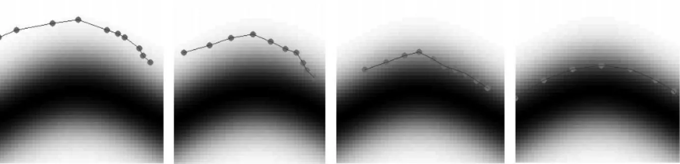
Figure 2.6 : Three examples of simple images with edges in different directions (left), corresponding adaptive meshes by spatial convolution filtering approach (middle), and corresponding adaptive meshes by geometric approximation approach (right) ... 15
Figure 2.7 : Geometric representation of deformable models ... 21
Figure 2.8 : Some iterative steps for parametric curve evolution to fit an edge ... 23
Figure 2.9 : Level set function of a curve ... 25
Figure 2.10 : Example of topology changes of the contour for ϕ function ... 26
Figure 2.11 : Manual initialization on a MR image (left) and final segmentation result (right) .... 28
Figure 2.12 : Simple model initialization on a MR image (left) and final segmentation result (right) ... 29
Figure 2.13 : Part of GVF fields and centers of divergence marked by circles [97] ... 29
Figure 2.14 : (a) An example of a binary feature map, (b) the derived EPGVF vector field, and (c) the segmented force field enclosed by the two dark thick contours ... 30
Figure 2.15 : Original image (left), computed VFC field (middle) and the estimated external energy of the VFC field (right) ... 31
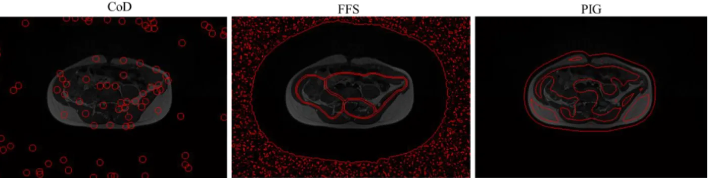
Figure 2.16 : Three different automatic initialization methods on a MR image; center of divergence (CoD) method (left), force field segmentation (FFS) method (middle), and
Poisson inverse gradient (PIG) method (right) ... 31
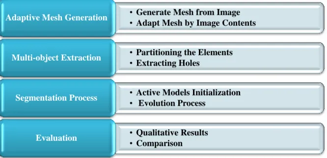
Figure 3.1 : Summary of general methodology presented in this thesis ... 37
Figure 4.1: Initial triangular mesh corresponding to original image pixels ... 38
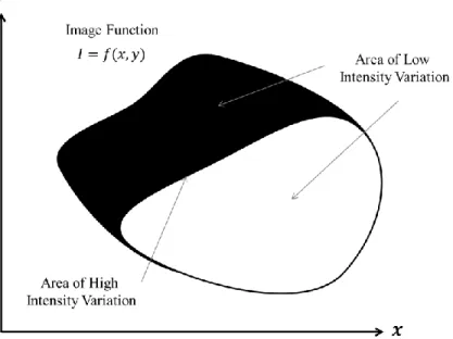
Figure 4.2 : Image 𝐼 as a function of intensity values in a global coordinate system (𝑥, 𝑦) ... 40
Figure 4.3 : Changing coordinate system and using proper neighborhood for Hessian computation ... 42
Figure 4.4 : Illustration of non-maximum suppression when the edge is blurry. The edge strengths are indicated both as colors and numbers. ... 44
Figure 4.5 : Picking a proper neighborhood for the pixel in the center according to its edge direction ... 44
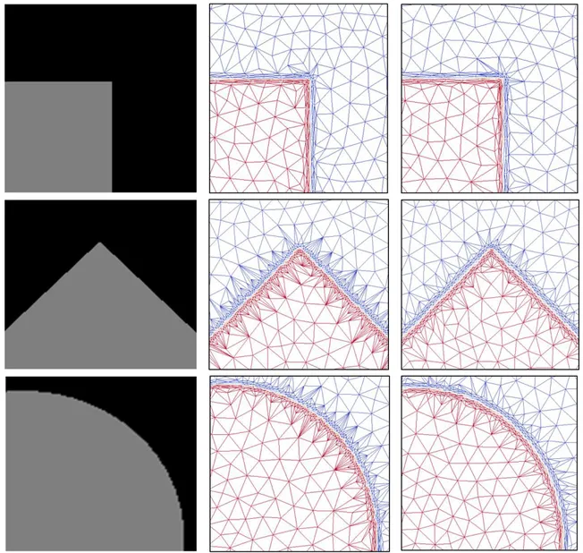
Figure 4.6 : Original images (top) and the corresponding adaptive meshes generated based on proposed metric construction (bottom) ... 47
Figure 4.7 : (A) Original MR image; (B) Adaptive mesh of the same image; (C) Zoom on the highlighted part in (B) ... 47
Figure 4.8 : Bimodal histogram of the element size for the mesh at the top and the result of selecting two different threshold values and removing the region elements from the mesh . 49 Figure 4.9 : (a) Original MR image (b) The corresponding adaptive mesh of the image (c) Extracting boundary elements (d) Identifying holes by locating boundary edges ... 50
Figure 4.10 : Various status of produced holes after identifying boundary edges of the mesh ... 51
Figure 4.11 : An example of creating a vector list for a given mesh edge set ... 53
Figure 4.12 : The schematic description of the algorithm for extracting the holes with an example ... 54
Figure 4.13 : Example of a B-spline curve with control points and corresponding basis functions ... 55
Figure 4.14 : Original MR image and its extracted sets of points (top) and overlay constructed curves onto the original image (bottom) ... 56 Figure 4.15 : Example of vector field kernel with radius 𝑅 and its related terms... 58 Figure 4.16 : Several closed active contours initialized on a MR image (left) final segmentation
result for detecting the true boundary of the organs in the image (right) ... 59 Figure 5.1 : Original images containing single objects for testing Hessian reconstruction
algorithms and their corresponding anisotropic adaptive meshes ... 61 Figure 5.2 : Zoom-in on resulting adapted meshes constructed based on three methods; the
approach by Farid & Simoncelli (left), the QF approach (middle), and our proposed approach (right) ... 62 Figure 5.3 : Element skewness on the adapted mesh obtained by the QF approach for axis-aligned
and non-axis-aligned edge directions ... 63 Figure 5.4 : Element skewness on the adapted mesh obtained by our proposed approach for axis-aligned and non-axis-axis-aligned edge directions ... 63 Figure 5.5 : Extracting the anisotropic elements (aspect ratio ≥ 2) from resulting meshes for the
three approaches for the Circle example and their corresponding histograms ... 65 Figure 5.6 : Anisotropic adaptive meshes constructed based on the three mentioned approaches
for the given MR image of the human trunk ... 66 Figure 5.7 : Extracting anisotropic elements (aspect ratio ≥ 2) from resulting meshes for the three
approaches for a MR image and their corresponding histograms ... 67 Figure 5.8 : Original MR image at the top and three mesh-based representations (isotropic, QF,
proposed method) and their corresponding reconstructed images ... 69 Figure 5.9 : Image reconstruction error over different types of adaptive meshes with different
sizes ... 70 Figure 5.10 : Comparison between QF method and proposed method on a series of MR images 71 Figure 5.11 : Original MR images of a human arm (left) Multiple active contour initializations
Figure 5.12 : Original MR image of human trunk sections (left) Multiple active contour
initializations (right) ... 73
Figure 5.13 : Comparison of automatic initialization on a MR image (example 1) ... 75
Figure 5.14 : Comparison of automatic initialization on a MR image (example 2) ... 75
Figure 5.15 : Comparison of automatic initialization on a MR image (example 3) ... 76
Figure 5.16 : Comparison of automatic initialization on a MR image (example 4) ... 76
Figure 5.17 : Comparison of automatic initialization on a MR image (example 5) ... 77
Figure 5.18 : Comparison of automatic initialization on a MR image (example 6) ... 77
Figure 5.19 : Evolving the initial contours to obtain final segmentation. Initial contours in red (left) Segmentation results in green (right) ... 79
Figure 5.20 : Comparison of segmentation result corresponding to initialization in figure 5.13 .. 81
Figure 5.21 : Comparison of segmentation result corresponding to initialization in figure 5.14 .. 81
Figure 5.22 : Comparison of segmentation result corresponding to initialization in figure 5.15 .. 82
Figure 5.23 : Comparison of segmentation result corresponding to initialization in figure 5.16 .. 82
Figure 5.24 : Comparison of segmentation result corresponding to initialization in figure 5.17 .. 83
Figure 5.25 : Comparison of segmentation result corresponding to initialization in figure 5.18 .. 83
Figure 5.26 : Original image of human lumbar spine, its model initialization, and segmentation (top), selected initialization and segmentation of intervertebral disks (bottom) ... 85
Figure 5.27 : Initial contour for an intervertebral disk (left), comparison between our segmentation in green and manual segmentation in white (right) ... 86
Figure 5.28 : Graph of Dice similarity results for all dataset ... 87
Figure 5.29 : Original image (left) and its proposed initialization with white contours superimposed on it to indicate the missing parts (right) ... 89
Figure 5.30 : The other three methods also failed to capture the bone structures in the example image in figure 5.27 ... 90
LIST OF SYMBOLS AND ABBREVIATIONS
MRI Magnetic resonance imagingMRF Markov random field EM Expectation maximization FCM Fuzzy c-means
CT Computed tomography
OORT Object-Oriented Remeshing Toolkit QF Quadratic Fitting
GVF Gradient Vector Flow CoD Center of Divergence FFS Force Field Segmentation PIG Poisson Inverse Gradient VFS Vector Field Convolution DSC Dice Similarity Coefficient
CHAPTER 1
INTRODUCTION
1.1
Context
Magnetic resonance imaging (MRI) has become a useful diagnostic tool in numerous fields of biomedical by providing high-resolution anatomic information on human soft tissue [1]. This imaging modality is non-invasive and does not require ionizing radiation. The scanner (figure 1.1) uses the property of nuclear magnetic resonance to create images. When the human body (which is mostly water) is placed in a strong magnetic field, the protons in the hydrogen atoms tend to align themselves with the field and result in a net magnetization of the body. This net magnetization can be pushed away from equilibrium by selectively exciting regions within the body with radio waves at an appropriate frequency. When eventually it returns to equilibrium (relaxation) it generates a radio-frequency electromagnetic signature, which can be measured and analyzed. MR imaging is able to provide high contrast sensitivity for visualizing differences among the tissues in the body because there are several sources of contrast. The contrast in an MR image is controlled both by the characteristics of the externally applied excitation and also the intrinsic properties of the tissues, which affect the relaxation times. Therefore these flexible characteristics of MR images allow varying the contrast between different tissues and highlighting various components in order to reveal fine details of the anatomy [2].
The problematic properties of MRI are intensity inhomogeneity and noise, which arise from the limitations of imaging devices. Due to the presence of this non-uniformity in the image, the intensity varies in different parts of the same tissue within the image. Although this is an imperceptible issue for a human observer, some image analysis methods which are sensitive to intensity variations, such as segmentation, encounter difficulties in identifying tissues based only on pixel intensity. It is very hard to rectify intensity inhomogeneity and noise from MR images because the non-uniformity patterns vary from patient to patient and from slice to slice. There are many methods that have been proposed for correcting the intensity inhomogeneity in MRI [3], but it is still not a completely solved problem, and we have to tackle this obstacle in the segmentation process. It is worth pointing out that intensity inhomogeneity correction and segmentation are two connected procedures and improvements in segmentation can boost non-uniformity correction. According to [3], there are some approaches for inhomogeneity correction which are segmentation-based methods. They try to merge two procedures so that they benefit from each other, simultaneously, in order to yield better segmentation and inhomogeneity correction.
Due to the distinctive characteristics of MRI, it plays a supplementary role in disease management from diagnosis to treatment planning and progress monitoring. Moreover, the creation of 3D patient-specific models out of these images for simulation purposes is becoming a beneficial application. Clinical interpretation of these medical images including segmentation, identification, and analysis of anatomical structures is an essential task which, for images with complicated shape and topology, is very challenging. Unlike traditional medical image analysis which has focused on a single organ or tissue applications, recent technological advances have brought increasing interest in simultaneous analysis and multi-object segmentation of medical images. Despite extensive research and methodological advances, there are still several issues that remain to be solved, and there is a high demand for a widely applicable automatic segmentation and classification technique which is able to handle all anatomical structures. New algorithms and technologies need to be investigated to meet these demands while preserving overall performance.
1.2
Motivation
MR image segmentation which is the process of extracting anatomically significant regions from the image is a challenging and important task in MR image analysis. Moreover, there is a growing need for automatic segmentation of multiple organs and complex structures from this medical imaging modality. Segmentation of multiple objects should provide a decomposition of the image into several components without overlap between the segmented regions.
In literature dealing with MR image segmentation, the region-based approaches which are looking for intensity similarities and try to group pixels into coherent regions, are sensitive to noise and non-uniformity in the input image. The edge-based approaches where use only the intensity discontinuities to determine region boundaries are challenging to group the edge information into a coherent closed contour. The atlas-based techniques which provide prior information for MRI segmentation can be problematic for complicated structures with anatomical variability. A class of variational methods known as deformable models has a great potential to confront MR multi-object segmentation challenges. These model-based techniques are designed to determine region boundaries using closed parametric curves that deform under defined force terms such that the curves are attracted to the image features (e.g. edges) while maintaining internal shape constraints. The main reasons why they are favored in MR image segmentation related to their robustness to noise and spurious edges, mathematical consistency, and sub-pixel accuracy. However they still have an important limitation which is that they are sensitive to initial position and shape of the model. An unsuitable initialization may provide failure to capture the true boundaries of the regions.
On the other hand, a useful aim for an automatic multi-object MR segmentation is to provide a model which promotes understanding of the structural features of the distinct objects within the MR images. However, the lack of connectivity of edge point features is a major limitation to aggregate edge points into a coherent closed curve for every distinct object and obtain initial models automatically only from edge points. Therefore we have to find richer information that is available from edges. The current automatic initialization methods which have used different descriptors such as gradient vector flow or Poisson inverse gradient are not completely successful in extracting multiple objects from MR images. But, the improvement trend of the results by
using higher level descriptions indicates that, providing more abstract level of information enhance the performance of the automatic initialization of the model.
In this regard, anisotropic adaptive meshes seem to be a potential solution to the aforesaid limitation. Mesh-based image representations facilitate the use of non-uniform sampling and have proven beneficial in many image analysis applications. To generate a mesh model of an image, the image domain is partitioned into a set of elements and then over each element an approximating function is constructed. Anisotropic mesh adaptation uses edge and gradient information of an image to provide a sort of structure tensor which is defined as a symmetric and positive semi definite matrix to modify the elements size and orientation in a specific manner. This structure tensor has two orthogonal eigenvectors and the corresponding eigenvalues which can be used to reveal more robust and accurate information about edge structure and orientation. Eigenvectors point in the direction orthogonal across the local edge, with the eigenvalues indicating the strength of the directional intensity change. Furthermore, the eigenvalues can be used as descriptors of local structure as it is shown in figure 1.2.
Figure 1.2 : Understanding local structure based on eigenvalues where E is the change of intensity for a small shift
Accordingly, anisotropic adaptive meshes constructed from MR images contain higher level, abstract information about the anatomical structures of the organs within the image retained as the elements shape and orientation. Adaptive mesh strategies try to specify metric tensors based on edge points information to control mesh elements characteristics so that they can align with the boundaries of the objects within the image. Existing methods for constructing metrics out of image features have a practical limitation where manifest itself in inadequate mesh elements alignment to inclined edges in the image. Therefore, we also have to enhance metric computation technique in mesh adaptation process to provide a better mesh-based representation. As we can provide a better mesh element alignment to the boundaries of the objects in the image, we may enhance the multi-object extraction process afterward.
Based on these insights, this thesis is going to introduce a new segmentation approach by integrating adaptive mesh generation techniques and deformable models to delineate the geometric structure of different structural objects in MR images.
In this research project, we have mainly focused on 2-dimensional MR images of the human trunk and try to segment all structural organs and tissues in these images. Since this is a very challenging and sophisticated case to handle, we expect our approach to be readily generalizable, and the proposed algorithms to be applicable to other kinds of MR images, thereby having an impact in the field of biomedical engineering.
1.3
Organization
Following the above introductory chapter, this thesis is organized as follows.
Chapter 2 provides relevant literature on three main topics. The first topic is about mesh concepts, mesh generation and adaptation techniques, and mesh-based image representation methods. The second topic is related to MR image properties and existing segmentation techniques for MR images with more details on deformable models as state-of-the-art methods. And the third one reviews current methods for multi-object medical image segmentation. The existing methods in each field are discussed with their advantages and limitations which are going to be addressed in the proposed methodology.
Chapter 3 summarizes the limitation of the existing approaches and presents general and specific objectives of the research project to address those limitations and also provide an overview of the proposed methodology.
Chapter 4 provides the details about the proposed methodology for developing a new mesh-based method for multi-object MR image segmentation.
In chapter 5, experiments and results are discussed. Finally, in chapter 6, conclusions and future research directions are presented.
CHAPTER 2
BACKGROUND & LITERATURE REVIEW
In the three sections that follow, we review the relevant literature to provide a clear understanding about challenges and opportunities in multi-object MR image segmentation towards our general methodology. First we provide a brief introduction to the mesh generation and mesh adaptation process along with literature review addressing the mesh-based image representations and their applications in medical image analysis including segmentation. Since the anisotropic adaptive mesh will be used to provide a roughly representation of multiple objects in the image, then we need to employ a segmentation technique to obtain the exact boundaries of the objects. In this regard we survey various segmentation techniques by emphasizing on active contour model as great candidates for segmenting multiple objects from MR images. The advantages of active contours and their limitations are discussed and the methods which address these limitations are investigated.
2.1
Mesh Generation and Adaptation
A mesh is a discretization of a continuous domain into simple elements such as triangles or quadrilaterals in two dimensions. The elements and their connectivity express the geometry and topology of the spatial domain. The shape and orientation of the elements affect both efficiency and accuracy of the mesh-based methods in scientific applications [4].
Generating meshes can be done in two different manners. Structured methods generate meshes with regular connectivity where all the vertices have the same number of neighbors, and all interior vertices are topologically alike (grid of quadrilaterals in 2D shown in figure 2.1). Structured meshes provide simplicity and easy data access, but they have lower geometrical flexibility. On the other hand, unstructured methods generate meshes with irregular connectivity where the number of neighbors may vary for different vertices (set of triangles in 2D shown in figure 2.1). Unstructured meshes are more costly to access, but they offer geometrical flexibility and more convenient mesh adaptivity for complicated domains.
Figure 2.1: Different types of meshes structured (left) and unstructured (right)
Since the domains that are studied in this research are medical images and they usually contain complicated structures, unstructured meshing methods are chosen over structured methods. Mesh adaptation refers to the modification of an existing mesh as to conform to physical features of the domain. The goal of these modifications is to achieve higher resolution of the domain features and lower overall computational time for respective applications [5-9].
Mesh adaptation methods try to modify the meshes by controlling the size, shape, and orientation of mesh elements throughout the domain and in this regard, they can be categorized into two types; isotropic vs. anisotropic.
Traditionally researchers have focused on isotropic mesh adaptation where only the size is specified for mesh element modification, and there is no stretching and orientation. Therefore, the triangles (mesh elements) in the result mesh are close to equilateral (figure 2.2). This can only be optimal if the gradients of the domain features are almost equal in all spatial directions. The alternative approach is an anisotropic mesh adaptation in which the mesh modifications are controlled to simultaneously adjust the size, shape, and orientation of mesh elements [9-13]. Thus, if the features of the domain are highly directional and the variation in one direction is more significant than the others, the triangles in the resulting mesh are stretched and aligned with directional properties (figure 2.3).
Figure 2.2: Size specification map and the corresponding isotropic mesh adapted based on the specified sizes [10]
Figure 2.3: Anisotropic map of a domain and the corresponding anisotropic mesh adapted based on the specified size, stretching and orientation [10]
Since the domain features studied in this project are the edges from the outline of the objects in the image and they are strongly directional, an anisotropic adaptation approach is chosen over an isotropic one. In the following, more details on anisotropic mesh adaptation are provided.
2.1.1 Anisotropic Mesh Adaptation
As mentioned before, the idea of mesh adaptation is to modify the mesh according to the domain features by controlling size and orientation. As a result, in areas of high variation in the domain, elements are fine and highly stretched, and in areas of low variation, elements are coarse and more regular. In this regard, the concept of metric is used to specify the mesh size in different directions and orientation. This is also called metric-based anisotropic adaptation.
Metric Notion
2.1.1.1
A Metric is a function defined over a domain that maps any point in the domain to a 2 × 2 matrix (in 2-dimensions) and expresses how long and skinny the triangles should be and in which direction they should be oriented. In another word, at each point, a metric determines how distances and angles are measured.
Geometrically, distance can be measured by the dot product between two vectors which is symmetric, positive, and definite. In 2 × 2 Euclidean space, for two vectors 𝑢 and 𝑣 the dot product is indicated in Eq. 2-1 and the length of a segment 𝑎𝑏 is given by Eq. 2-2.
〈𝑢⃗ , 𝑣 〉 = 𝑢⃗ 𝑡 𝑣 (2-1)
ℓ(𝑎, 𝑏) = √ 𝑎𝑏𝑡⃗⃗⃗⃗ 𝑎𝑏⃗⃗⃗⃗ (2-2)
In Euclidean metric space, the dot product is generalized by introducing a 2 × 2 symmetric positive definite matrix as ℳ = [𝑎 𝑏
𝑏 𝑐].
In this space, the distance definition is shown in Eq. 2-3 and length of the segment 𝑎𝑏 is given by Eq. 2-4.
〈𝑢⃗ , 𝑣 〉ℳ = 𝑢⃗ 𝑡 ℳ𝑣 (2-3)
In the context of mesh adaptation, a Riemannian metric space defined by 𝑀 = (ℳ(𝑥))𝑥∈Ω represents ℳ as a Riemannian metric over the space of parametrization Ω. To consider the variation of the metric along the segment 𝑎𝑏 the length is computed using the straight line parametrization in domain Ω with an integral formula as in Eq. 2-5.
ℓℳ(𝑎, 𝑏) = ∫ √ 𝑎𝑏𝑡⃗⃗⃗⃗ ℳ(𝑎 + 𝑡𝑎𝑏)𝑎𝑏⃗⃗⃗⃗ dt 1
0
(2-5)
Where 𝑡 ∈ [0,1].
Geometric Representation of Metrics
2.1.1.2
In the above equations, the metric ℳ which is also called a metric tensor, has geometric representation in the form of an ellipse [14]. Since this metric tensor is symmetric, it is diagonalizable and can be decomposed as indicated in Eq. 2-6.
ℳ = ℛ Λ ℛ𝑡 Λ = [𝜆01 𝜆0
2] ℛ = (𝑒⃗⃗⃗ , 𝑒1 ⃗⃗⃗ ) 2
(2-6)
where ℛ is an orthonormal matrix containing the eigenvectors of ℳ that represent the two axes of the ellipse and Λ is a diagonal matrix containing the eigenvalues of ℳ specifying two lengths of the ellipse axes as ℎ𝑖 = 𝜆−1 2𝑖 ⁄ as shown in figure 2.4.
Geometric representation of metric tensors by ellipses provides a convenient way to visualize the size, stretching, and orientation over the domain for mesh generation and adaptation process.
Mesh Adaptation Scheme
2.1.1.3
There are many software systems for performing anisotropic mesh adaptation and the more recent ones are, Gamanic3d [15], Tango [16], Mesh Adap [17], OORT [18], Feflo.a [19], and MAdLib [20].
The OORT (Object-Oriented Remeshing Toolkit) which was developed by Julien Dompierre and Paul Labbe is the one that has been chosen for this project. The capacity of this tool for metric-based anisotropic mesh adaptation has been shown in [21]. The adaptation process in OORT is performed iteratively as it is shown in figure 2.5.
In each iteration, any local mesh modification (including moving vertices, swapping, refining, and decimating edges of the elements) is done to satisfy the metric. The final result is a unit mesh in predefined Riemannian metric space in which all elements are quasi-unit while they are adapted and anisotropic in the Euclidean space.
2.2
Mesh-based Image Models
In recent years, researchers have presented numerical simulations in the biomedical field in order to investigate the impact of medical treatments in different areas including cardiology, neurology, orthopedic surgery, etc. Many of these simulators are constructed based on medical images by generating structured or unstructured meshes from the images. Then through an adaptation process, the initial mesh is deformed to follow desirable features within the image. In the scope of this research, desirable features of an image are considered as all the edges in the image that represent boundaries of different regions (in particular, distinct anatomical tissues) within the image. Therefore the process of mesh deformation to conform to the edges involves changing mesh elements size and orientation to align element edges with the boundaries of the regions. As mentioned before, although structured meshes can produce high-quality models, the advantages of using unstructured meshes include generating meshes with fewer elements and the ability to conform better with image features [23, 24]. In this regard, we are going to focus on generating unstructured meshes and anisotropic adaptation processes applied on these meshes. Many of these methods are considered as sampling methods which try to find desired sample points first and then connect the points to construct a mesh [25-35] and a few methods start from an initial mesh and then try to adapt the mesh according to the image content [22, 36-38]. Ramponi and Carrato [33] have introduced non-uniform grids using an irregular sampling scheme based on measuring the change in gray-level values. Yang et al. [31] have represented an adaptive mesh generation technique by placing the mesh vertices using the classical Floyd-Steinberg error diffusion algorithm and then using Delaunay triangulation to connect the vertices. The resulting mesh contains small elements where the gray-level variation is high and large elements in low variation regions. Demaret et al. [27, 28] have proposed an image approximation scheme for the
purpose of image compression which starts with all image points and then removes less significant pixels in a greedy way to reach the smallest reconstruction error. Adams et al. [25] have presented an effective framework based on the greedy point removal scheme of Demaret et al. and the idea of the error diffusion scheme of Yang et al. in order to replace the initial mesh of all image points with a good subset of those sample points. This would provide a flexible tradeoff between mesh quality and computational and memory complexity. Sarkis and Diepold [36] have combined a Binary Space Partition and clustering scheme to present a new method for approximating an image with a mesh. They cluster the image area into a few triangles and try to model the intensity variation inside each triangle and reconstruct the gray level values of pixels lying within. If a triangle's equation does not have the ability to reconstruct those pixel values, it is subdivided recursively based on a predefined threshold. Bougleux et al. [37] have shown that anisotropic sampling and triangulation are crucial to improve image approximation. They have proposed a progressive geodesic meshing that defines geodesic distance using a Riemannian Fast Marching to force the triangulation to follow the anisotropy of the image. However, in their method, the metrics are constructed using first order derivatives which make the eigenvalues physically meaningless. On the other hand, Riemannian metric tensors have been used to control the anisotropic adaptation of meshes. These metric tensors in the case of images are constructed based on second order derivatives of the intensity of the image at every pixel. Several approaches have been presented for the computation of second order derivatives of images. Vallet et al. [39] have compared different methods such as: Double linear fitting (DLF) [40], Simple linear fitting (SLF) [41], Double 𝐿2-projection (DL2P) [42], and Quadratic fitting (QF) [43]. The common feature of all these methods is that they try to find an approximation of the image function at each pixel and then the partial derivatives of these functions will be derived to construct the Hessian matrix for all pixel intensities. Among these second derivatives recovery methods, they suggest that, the QF method which fits a least-square quadratic polynomial on a two neighborhood levels patch is more robust and more accurate. O. Courchesne et al. [22] have applied the QF method on MRI images to compute a Hessian matrix and construct metric tensors for mesh adaptation processes. The result in figure 2.6 shows that this approach only works perfectly for edges in vertical and horizontal directions and for other directions it can align element edges with the oriented boundaries but not as perfectly as in the main two directions.
Several methods have been proposed for computing image derivatives using special convolution filters such as Steerable filters [44] and least-squares polynomial smoothing [45]. Farid and Simoncelli [46, 47] have provided a discrete representation of their continuous differentiation scheme as some optimized differentiating filters which are commonly used in practice. Their method has demonstrated more accuracy in estimating local orientation in images. However, the result of constructing a metric based on the image derivatives is shown in figure 2.6 which only gives proper alignment in horizontal and vertical directions and fails to be aligned in other directions.
Figure 2.6 : Three examples of simple images with edges in different directions (left), corresponding adaptive meshes by spatial convolution filtering approach (middle), and
In summary, the above literature review indicates that the main limitation of the existing approaches for anisotropic mesh adaptation is their inadequate alignment for non-axis aligned edge directions. Therefore we need to construct an adaptive mesh for a given image in which elements of the mesh become aligned with the boundaries of the objects in any directions.
As mentioned before, we want to incorporate anisotropic mesh adaptation and segmentation methods to present an automatic multi-object segmentation technique. In this regard we survey various segmentation techniques for MR images in the following section.
2.3
MRI Segmentation Techniques
In this section, we review some of the current methods in MRI segmentation and the state-of-the-art related to the proposed segmentation framework. A large and growing body of literature has been published which can be divided into three main categories: classification-based, region-based and contour-region-based techniques. In the following sections, we discuss the characteristics, advantages, and disadvantages of these methods.
2.3.1 Classification-Based Techniques
In classification-based methods, segmentation is the process of classifying pixels into certain tissue classes based on some specific criteria. One class of techniques in this category is statistical pattern recognition models, which have been applied extensively in MRI segmentation [48]. A mixture model is used to model the probability density function of tissue classes. A set of features based on pixel information is provided in order to measure the probability of pixels belonging to each class. Generally, to characterize the variation of each pixel feature, a class conditional probability distribution is needed which is generally unknown [49]. In supervised approaches, these distributions will be provided based on the tissue regions identified by the user. In statistical clustering [50], they can be approximated automatically based on the image data in an iterative way. On the other hand, some of the statistical methods, which are considered as parametric methods, assume that the conditional distribution of classes is known and often model
them as a mixture of Gaussians [51]. Many statistical methods assume that the number of tissue classes and a priori probability of their occurrence are provided prior to the segmentation process. Then, in order to estimate a posteriori probability, the Bayes rule is employed, and pixels are assigned to the class with highest a posteriori probabilities [52]. Markov random fields (MRF) are introduced to incorporate local contextual information which allows neighbourhood pixels to affect segmentation. MRF also provides reliable information to model the possible neighbourhood for each tissue class [53]. A recent study shows that MRF regularization allows modelling the spatial interaction in neighbourhood space [54]. Another implementation of statistical clustering for tissue identification is based on a 3-step expectation maximization (EM) algorithm [55, 56]. This iterative procedure also assumes tissue classes as a mixture of Gaussians and creates a model with MRF regularization in order to reduce segmentation errors arising from intensity inhomogeneity and noise. Although statistical techniques result in a significant improvement in MRI segmentation, they are still not powerful enough to yield automatic and accurate segmentation, in the general case [57].
A popular class of pixel clustering methods is based on a fuzzy clustering technique, derived from the fuzzy c-means (FCM) algorithm [52]. The FCM and its derivatives have been found very successful in medical image segmentation particularly in those cases where distinctive decisions have to be made. Clustering algorithms allow image pixels to be grouped together based on similarity of the description features. Unlike hard c-means algorithms which assign an absolute membership to one of the classes, the FCM algorithm assigns a degree of membership to each of the classes. Some adaptive methods based on FCM have been applied to MRI segmentation [58, 59]. These methods implement a modified objective function for FCM to model the variation in intensity value and help to amend the intensity inhomogeneity problem. However, they do not pay attention to spatial context between pixels because the procedure is done in the feature space and this limitation makes them sensitive to noise and image artefacts. Some alternative approaches have been proposed to consider spatial constraints and reduce errors caused by noise [58, 60], but they induce a higher computational complexity and are time-consuming.
Some recent studies [61, 62] have presented visual features for capturing spatial context for detection and localization of anatomical structure in CT images, and they plan to extend their technique to MR images. They have incorporated those features within a random decision forest
classifier. A random forest [63] is a collection of randomly trained decision trees. Decision trees were once very popular, but researchers have stopped using them because they suffer from the over-fitting problem and consequently they don't tend to generalize and provide well prediction. After coming along the idea of bias-variance trade-off, it was found that even though trees have very high variance in their predictions, if you make many trees and average them, you can get rid of the variance and build one of the most powerful classifier called random forest. A Random forest is a kind of ensemble model, and the algorithm simply takes the trees, sums them and divides by the number of trees. The algorithm has two sources of randomness, one is the randomness of the input data, and the other one is the randomness in the features. Injecting such randomness improves generalization. So, by randomly choosing input data and features for different trees, each tree only sees a small part of the data and features. Each tree is correct but missing a lot of information, but when we average them, we get a classifier which is very near the truth. Just like the forest can be used for classification, it also can be used for regression. A split point is introduced which divides the data into two nodes, and then in each node, a linear model is fitted. The aforesaid techniques built upon randomized decision forests for detecting anatomical structures have been enriched with learned visual features which capture long-range spatial context. Although they have presented satisfactory result in the case of CT images and might be extendable to MR images, they have focused only on some specific human organs. In order to consider all organs and tissues and moreover to introduce general-purpose classifier, further generic features need to be defined.
2.3.2 Region-Based Techniques
Another way of describing the objects in the image is by determining the region they occupy. Usually, the pixels within an object have similar intensity or texture characteristics. Accordingly, region-based methods make efforts to identify homogenous regions in the image in order to segment various objects. Region-based techniques, unlike clustering approaches, try to embody spatial properties between pixels and neighborhood information. Thresholding [64] approaches are the simplest techniques which try to find a threshold value to differentiate between tissue regions in the image. Although these methods are computationally fast, in the presence of noise and intensity inhomogeneity, it becomes very difficult to determine thresholds accurately.
Another simple idea is to determine some seeds indicating different regions and let them grow until the entire image is covered [65, 66]. In this regard, for controlling the growing process, some rules or tools must be provided to check the similarity at each growth step. One class of region-based approaches which has been used for MRI segmentation is region growing. These methods start by locating the seeds in the image and check the neighborhood pixels with predefined homogeneity criteria to identify biological segments [67]. Most of these techniques are semi-automatic and rely on user interactions. Also, some automatic statistical forms of these methods have been proposed. They estimate local mean and variance for each pixel and try to find the best parameter via a minimization function, but in the general case, they encounter some difficulties in determining a proper homogeneity criterion in advance [68]. In this regard, an adaptive technique was proposed which attempts to learn the criteria automatically, based on the characteristics of the regions during the segmentation process [69].
Split and merge techniques are another set of region-based methods that operate on an image in a recursive way. They start with entire images and check intensity homogeneity, and if pixels are not all of a similar intensity, the volume is split into smaller sub-regions, and the same process is applied to sub-sections. In the merge step, the inverse direction is followed, and the small regions are joined together if they have enough similarity [70]. In the case of medical images, the major problem is when the image contains many small sub-regions with variable sizes which cause over-segmentation difficulties.
2.3.3 Contour-Based Techniques
Several attempts have been made to segment biological and anatomical objects in MR images by detecting their boundaries. This group of approaches is categorized as contour-based segmentation techniques.
A notable idea in the class of edge detection methods suggests combining Marr-Hildreth and morphological operators for edge detection and edge refinement in MRI segmentations [71]. Some other studies based on edge tracing, which is commonly used in image processing, try to extract edge information and trace the adjacent connectivity to represent the object boundaries [72]. Typically they are not applicable for segmentation problems on their own, because their
information is based on local intensity variations and may not always result in a closed form and connected boundaries. Some studies have been done to produce suboptimal results and also reduce computation time, but they are restricted to segmentation of large and well-defined structures [73]. Generally, these boundary-based methods tend to be sensitive to noise and image artefacts and may suffer seriously from over and under-segmentation due to the inaccurate threshold selection [74]. Some MRI segmentation approaches are based on the watershed algorithm. They choose to model MR images as topographic reliefs where intensity values of voxels determine the physical elevation. The watershed method subdivides the image into basic elements, called catchment basins and considers each one has a local minimum. By imagining a hole at each local minimum of the topographic relief, as the catchment basins are filled with water, the surface will be immersed starting from the basin which is associated to the global minimum. As soon as water flows from one catchment basin to another, a dam is built. In the end, the borders defined by the watersheds represent the segmentation result [75]. This semi-automatic segmentation method also suffers from an over-segmentation problem in the presence of noise and other artefacts [57]. The images have to be smoothed prior to the watershed operation in order to reduce this adverse effect.
In recent years there has been a considerable amount of literature on a group of contour-based methods known as deformable models. These methods have an increasing influence on medical image segmentation including MRI segmentation. Their distinctive properties, which are discussed in the following, make them state-of-the-art methods for MRI segmentation.
Deformable Models
2.3.3.1
Deformable models are used in a very large range of applications such as image processing, surgery simulation, computer animation, etc. Different models can be classified based on their contour representation as it is shown in figure 2.7. The difference between continuous and discrete representation is that in discrete form the geometry of contours is only known at finite sets of points. Continuous forms must be discretized for computational needs, but it is possible to compute normal and curvature along the whole curve.
Figure 2.7 : Geometric representation of deformable models
Continuous models have been used extensively for image segmentation while discrete models such as meshes are mostly used for object modelling. There are some advantages in using deformable models in medical images over other segmentation techniques. They are able to generate closed parametric templates from images in a smooth manner, making them robust to noise and spurious edges, and able to manage complex geometries and topology changes (curve splitting and merging). Moreover, they provide consistent mathematical descriptions, which can be used for subsequent applications. Continuous deformable models including active contours (2D) and active surfaces (3D) provide some closed curves or surfaces with the ability of expansion and contraction to fit the objects’ boundaries. There are two types of these deformable models: parametric and geometric.
2.3.3.1.1 Parametric Models
Parametric models represent deformable contour that are explicit in their parametric form during deformation. Mathematically, a deformable contour is a parametrized curve 𝐶(𝑠) = [𝑋(𝑠), 𝑌(𝑠)]; 𝑠 ∈ [0,1] where deformation is based on energy minimizing functions. Most of them are derived from snake models [76]. Snake energy formulation is based on internal and external forces as shown in Eq. 2-1:
Deformable Models Continuous Models Explicit Representation (Parametric) Implicit Represemtation (Geometric) Discrete Models Discrete Meshes Particle Systems
𝐸 = 𝐸(𝑖𝑛𝑡) + 𝐸(𝑒𝑥𝑡) (2-1) Internal energy manifests itself in the smoothness of the shape and is given by Eq. 2-2:
𝐸(𝑖𝑛𝑡) = ∫ 𝛼|𝐶1 ′(𝑠)|2+ 𝛽|𝐶′′(𝑠)|2𝑑𝑠 0
(2-2)
Where α and β control the tension and rigidity of contours respectively and 𝐶′(𝑠) and 𝐶′′(𝑠) are curve derivatives.
External energy consists of potential forces which usually involve forces derived from the image. The role of the external energy is to make the curve converge towards the edges and is given by Eq. 2-3:
𝐸(𝑒𝑥𝑡) = ∫ 𝐸𝑖𝑚(𝐶(𝑠)) 1
0
𝑑𝑠 (2-3)
𝐸𝑖𝑚 is the edge attraction function and represents the gradient of the image intensity function. Local minima of 𝐸𝑖𝑚 represent the situation where the snake and the edge conform to each other (figure 2.8). It is defined as Eq. 2-4:
𝐸𝑖𝑚 = 1
𝜆 |∇𝐺𝜎∗ 𝐼(𝑥, 𝑦)| (2-4)
Where λ is a chosen constant, 𝐺𝜎 is a Gaussian function with standard deviation σ, ∇ is the gradient operator, * is the image convolution operator, and 𝐼(𝑥, 𝑦) is a given gray-level image. So, the curve moves through the spatial domain of an image to minimize the following energy function (Eq. 2-5):
𝐸 = ∫ [12(𝛼|𝐶′(𝑠)|2+ 𝛽|𝐶′′(𝑠)|2) + 𝐸𝑖𝑚(𝐶(𝑠))] 𝑑𝑠 1
0
Figure 2.8 : Some iterative steps for parametric curve evolution to fit an edge
Many extensions have been proposed for medical image analysis including segmentation. The first use of parametric models in segmentation was proposed in [77]. The major limitations of their approach are that they can only provide accurate results if the initial curve is given close to the edge and they also detect some spurious edges as real edges of the structures. Although many modifications have been done to traditional snakes to overcome the initial condition and spurious edge problems, they all suffer from noise and other image artefacts due to the fact that they only use the gradients of the image. In order to solve this problem, one study [78] suggests using gradient vector flow (GVF) as a kind of region-based feature to form the external force. They alleviate the problems related to noise and are also able to handle concave objects. However, their method has some drawbacks. The generation of GVF needs intensive computations. Also, weak and strong edges create similar flow because only the gradient information affects the flow. Another problem of traditional snakes is convergence to local minima which makes them improper for noisy images. Another early study [79] suggests a different external force model. They first apply a Gaussian kernel for smoothing and then compute the edge map based on a gradient operator or Gabor filter. They improve the capture range, but this method requires prior information of the object in order to select the initial parameter and produce accurate results. Another research [80] indicates a different formulation of the energy function based on a mean shift technique in order to improve segmentation accuracy and computational efficiency, but it still has initial condition and parameter optimization problems. In addition, several issues still remain unsolved for parametric models such as topological changes, handling multiple objects, and convergence stability. Another class of methods known as geometric models is proposed to handle some of these limitations.
2.3.3.1.2 Geometric Models
Geometric models deform curves or surfaces implicitly as a particular level of a function and using an elegant formulation based on the object geometry. These models comprise two approaches; one is based on curve evolution theory [81] which uses geometric information such as curvatures and unit normal for curve deformation, and another one is based on level set methods which represent curves or surfaces as a level set of a higher dimension scalar function. After complete deformation, the parameterized model is computed.
In the first approach, the curves are parameterized and the energy function can be defined by adding an integral functional on the boundary and another integral functional inside the boundary. Then the contour that minimizes the energy function can be identified by an Euler-Lagrange equation. Let us consider the curve 𝑿(𝑠, 𝑡) = [𝑋(𝑠, 𝑡), 𝑌(𝑠, 𝑡)] where 𝑠 is any parametrization and 𝑡 is the time. The contour evolution towards the minimum is implemented by the gradient descent equation (Eq. 2-6):
𝜕𝑿
𝜕𝑡 = 𝑉(𝑘). 𝑁,⃗⃗⃗⃗ (2-6)
which moves the contour along the normal 𝑁⃗⃗ with the speed function 𝑉(𝑘).
In the level set approach [79, 82], a function represents the contour in implicit form and uses a contour of higher order; a 3D surface is used for 2D curves and a 4D hyper-surface for representing 3D surfaces. If Ω is the range of the contour model and function 𝜙: Ω × ℜ+ ⟶ ℜ is defined, the task is to analyze and compute deformation under a velocity field. This velocity can depend on position, time, geometry (normal and mean curvature) of the curve and the external physics. The curve is expressed with a function 𝜙 (figure 2.9) as Eq. 2-7:
𝑿 = {𝑥|𝜙(𝑠, 𝑡) = 0} (2-7)

![Figure 2.2: Size specification map and the corresponding isotropic mesh adapted based on the specified sizes [10]](https://thumb-eu.123doks.com/thumbv2/123doknet/2340086.33703/27.918.219.697.106.400/figure-size-specification-corresponding-isotropic-adapted-based-specified.webp)
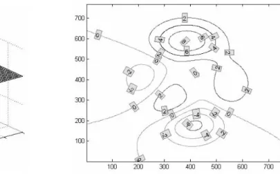
![Figure 2.13 : Part of GVF fields and centers of divergence marked by circles [97]](https://thumb-eu.123doks.com/thumbv2/123doknet/2340086.33703/47.918.206.710.727.961/figure-gvf-fields-centers-divergence-marked-circles.webp)