HAL Id: inserm-00610417
https://www.hal.inserm.fr/inserm-00610417
Submitted on 21 Jul 2011HAL is a multi-disciplinary open access archive for the deposit and dissemination of sci-entific research documents, whether they are pub-lished or not. The documents may come from teaching and research institutions in France or abroad, or from public or private research centers.
L’archive ouverte pluridisciplinaire HAL, est destinée au dépôt et à la diffusion de documents scientifiques de niveau recherche, publiés ou non, émanant des établissements d’enseignement et de recherche français ou étrangers, des laboratoires publics ou privés.
Appearance-based modeling for segmentation of
hippocampus and amygdala using multi-contrast MR
imaging.
Shiyan Hu, Pierrick Coupé, Jens Pruessner, Louis Collins
To cite this version:
Shiyan Hu, Pierrick Coupé, Jens Pruessner, Louis Collins. Appearance-based modeling for segmenta-tion of hippocampus and amygdala using multi-contrast MR imaging.. NeuroImage, Elsevier, 2011, 58 (2), pp.549-59. �10.1016/j.neuroimage.2011.06.054�. �inserm-00610417�
Appearance-based Modeling for Segmentation of Hippocampus and
Amygdala using Multi-contrast MR Imaging
Shiyan Hu*, Pierrick Coup´e, Jens C. Pruessner, and D. Louis Collins McConnell Brain Imaging Centre, Montreal Neurological Institute,
McGill University, Montr´eal, Qu´ebec, Canada H3A 2B4
*Corresponding Author, Shiyan Hu, Phone: (613) 5995397, E-mail: [email protected]
Abstract
A new automatic model-based segmentation scheme is presented that combines level set shape modeling and active appearance modeling (AAM). Since different MR image contrasts can yield complementary information, multi-contrast images can be incorporated into the active appearance modeling to improve segmentation performance. During active appearance modeling, the weighting of each contrast is optimized to account for the potentially varying contribution of each image while optimizing the model parameters that correspond to the shape and appearance eigen-images in order to minimize the difference between the multi-contrast test images and the ones synthesized from the shape and appearance modeling. As appearance-based modeling techniques are dependent on the initial alignment of training data, we compare (i) linear alignment of whole brain, (ii) linear alignment of a local volume of interest and (iii) non-linear alignment of a local volume of interest. The proposed segmentation scheme can be used to segment human hippocampi (HC) and amyg-dalae (AG), which have weak intensity contrast with their background in MRI. The experiments demonstrate that non-linear alignment of training data yields the best results and that multi-modal segmentation using T1-weighted, T2-weighted and proton density-weighted images yields better segmentation results than any single contrast. In a four-fold cross validation with eighty young normal subjects, the method yields a mean Dice κ of 0.87 with intraclass correlation coeffi-cient (ICC) of 0.946 for HC and a mean Dice κ of 0.81 with ICC of 0.924 for AG between manual and automatic labels.
1
Introduction
The hippocampus (HC) and amygdala (AG) are important parts of the limbic system and are located in the medial temporal lobe (MTL). While the HC plays an important role in learning and memory, the
AG seems to be more involved in regulating emotions and emotional memory, especially in association with fear. Both HC and AG contribute to regulate various autonomic and metabolic functions, e.g. the hypothalamus-pituitary adrenal axis. Recently, the HC and AG have received considerable attention due to their involvement in the onset and progression of neurological and neurodegenerative diseases (Mori et al., 1993). For example, hippocampal volume changes have been established as markers of early stage Alzheimer’s disease and in patients with temporal lobe epilepsy (Wang et al., 2005; Duzel et al., 2005).
Current approaches in the study of characterizing the hippocampus volume and segmenting the hippocampus are heavily reliant in vivo imaging techniques such as magnetic resonance imaging (MRI). Although manual segmentation of the HC is considered highly accurate, it suffers from some serious drawbacks: manual segmentation is time consuming, requires anatomical expertise, and may have important intra and inter-observer variability. These disadvantages have motivated researchers to develop automatic segmentation techniques (Pal and Pal, 1993; Hogan et al., 2000; Fischl et al., 2002). However, poor image contrast, noise, and missing or diffuse boundaries make the automation difficult. This is especially true when trying to distinguish the HC from the adjacent gray matter structures, due to weak image intensity contrast between the HC and surrounding structures. To overcome those difficulties, model-based methods are widely used in image interpretation. A comprehensive overview of model-based segmentation methods can be found in review of Rousson (Rousson, 2004). Recently, many researchers use atlas-based methods to improve the segmentation accuracy. These techniques make the use of expert annotations in the form of prior information to assist in providing automatic segmentations (Fischl et al., 2002; Shattuck et al., 2008). Multi-atlas based methods are more effective in comparison with other atlas based approaches (Heckemann et al., 2006; Aljabar et al., 2009). For those techniques, the quality of the registration methods and the selection of the templates will directly affect the segmentation performance. Also, the atlas-based techniques don’t explicitly incorporate the structure’s shape information into the segmentation.
To integrate the shape information into the segmentation, PCA-based or appearance model-based strategies, which use shape variability as constraints on segmentation, are widely used in human brain subcortical structure segmentation. Tsai (Tsai et al., 2003) proposed a shape model to segment med-ical images, where a level set method, based on the work of Osher and Sethian (Osher and Sethian, 1988), was used to represent the shapes of the structure of interest. The approach was demonstrated to have less computational complexity and be robust to noise. However, Tsai used only the prior shape knowledge in segmentation, not taking full advantage of the information available such as texture.
Cootes et al. (Cootes et al., 1998), have used image texture in segmentation where a landmark-based active appearance model (AAM) was developed to capture the statistical characteristics in terms of shape and gray-level information from the training images. His model was shown to fit shape contours rapidly in new test images. Nevertheless, in (Cootes et al., 1998), shapes were described by a set of control points or landmarks manually placed on each image. Thus, labeling landmarks/control points in the training images is important since the choice of landmarks influences the model significantly. Incorrect landmarks may result in generating an invalid shape during segmentation (Davies, 2002). In addition, manually determining point locations and point correspondences during training is time consuming and tedious. Recently, some automated methods were developed to establish point corre-spondence for an appearance model developed within a Bayesian framework to improve the robustness of the algorithm (Patenaude et al., 2011). Also landmark-based shape representation suffers from some mathematical problems, such as numerical instability, and difficulty in handling topological changes, to which the level-set techniques have shown good performance (Tsai et al., 2003). Therefore, it is of interest to study the combination of those two techniques (Level-Set + AAM) in image segmentation. One of the first published methods to combine level-set shape representation and statistic gray information into the segmentation could be found in (Yang and Duncan, 2004), where a 3D segmen-tation method was developed with joint shape-intensity prior models using level sets. This method showed good performance in segmenting brain sub-cortical structures. However, Yang’s imaging model assumed a constant gray level within the object to be segmented. This is not the case in the algo-rithm proposed here. We use a generative model that is capable of synthesizing an image with a more realistic, non-homogeneous texture for the hippocampus, amygdala, and the surrounding anatomical region. The objective function used in our optimization is based on the voxel-based intensity difference between the synthesized image and test image.
In our previous work in image segmentation, we combined level-set shape modeling and appearance modeling to identify the lateral ventricles from MR data (Hu and Collins, 2007). We propose two significant improvements on our previous appearance modeling method. First, multi-contrast images such as T1, T2, and PD MR images have complementary intensity relationships and can help in structure segmentation but their informative value may vary from subject to subject. To overcome the limitation of the fixed weights used in our previous work (Hu and Collins, 2007), we proposed to estimate the contribution of each image contrast during the segmentation process, where the optimum weight of each modality image is based on the correlation coefficient of the synthesized image and corresponding test image. For the model parameters corresponding to the shape and appearance
eigen-images to construct the synthesized appearance images, the least square (LS) search algorithm is adopted to find the optimum solution in the least square sense. Both search for the model parameters and weights of contribution are applied iteratively to minimize the difference between multi-contrast test images and the ones synthesized from the joint shape and appearance modeling. The proposed method has been tested on real 3D MR images to segment the HC and AG, and the results demonstrate that this new method is fast, accurate and robust. Second, appearance-based modeling requires alignment of all training data as a pre-processing step and the segmentation result is dependent on quality of these registrations. In our previous work (Hu and Collins, 2007), we registered all MRI volumes into stereotaxic space using an affine transformation that best aligned the whole brain (Collins et al., 1994). In order to improve the registration of the structures of interest (i.e., HC and AG), we compare the previous global linear brain registration with a local linear registration defined within a volume of interest (VOI) defined around the medial temporal lobe and a local non-linear registration defined in the same VOI. We show that the local linear registration yields better segmentation results than the global linear registration, and that the non-linear registration yields even better results.
The main contribution of this paper includes: 1) the proposed method pushes PCA techniques further to improve the segmentation performance; 2) multi-contrast images, i.e. T1, T2, and PD MR images, are incorporated into the segmentation procedure, and the contribution of each modality image is optimized during the segmentation; 3) since PCA-based techniques require that the structure to be segmented are pre-aligned, this paper explores the effect of the quality of registration methods on the segmentation accuracy; and 4) the algorithm is very fast and able to accurately segment a new subject.
2
Combined Shape and Appearance Modeling for Segmentation
The segmentation approach presented in this paper can be characterized into four processing stages: 1) image pre-processing, 2) level set shape modeling, 3) active appearance modeling, and 4) appearance model-based segmentation.
2.1 Image Preprocessing
Image pre-processing is the first step in image segmentation, and it is required before any training data is incorporated into the models or before any new image can be segmented. The goal of image pre-processing is to remove the variation in shape and image intensities due to the different coordinate
systems, head positions, image intensity non-uniformity or other artifacts, and to increase the similarity among the shapes compared and images. Image pre-processing includes the following basic steps:
i) Image intensity non-uniformity correction: We use the nonparametric method developed by Sled (Sled et al., 1998) to reduce intensity non-uniformity. The method iteratively estimates both the multiplicative bias field and the distribution of the true tissue intensities.
ii) Image registration: In order to account for different brain position, orientation and size with the volumetric data, we use three different registration techniques to align all image data together: (1) Linear registration: we linearly register all image data into the standard Talairach-like MNI stereotaxic space (Collins et al., 1994) and resample data onto a regular 1mm × 1mm × 1mm grid. (2) Local linear registration: this is done in a two-step process. We first align the whole brain (Collins et al., 1994), and second, we use the whole brain transformation as a starting point for a local linear registration of the VOI surrounding the HC and AG. (3) Non-linear registration: similar to the local linear registration, we first align the whole brain (Collins et al., 1994), and then use the whole brain transformation as a starting point to do non-linear reg-istration to an unbiased non-linear average template known as the ICBM152 2009c nonlinear asymmetric 1 × 1 × 1 mm template (known as mni icbm152 nl 09c asym and available from www.bic.mni.mcgill.ca/ServicesAtlases/ICBM152N lin2009) (Fonov et al., 2009; Fonov et al., 2011). The non-linear registration is done by Animal (Collins and Evans, 1997). To save time, the non-linear registration is estimated only within the region of interest surrounding the HC and AG. The linear and on-linear registration steps minimize size, orientation and position dif-ferences between subjects. After the registration, T1, T2, and PD images are aligned together in the standard MNI (Talairach-like) mni icbm152 nl 09c asym space.
iii) Intensity normalization based on a common volume of reference: Within the local HC VOI described above, we normalize the intensities to the range of 0 to 100. The formula for the normalization is: I−Imin
Imax−Imin×100, where Iminand Imaxare the minimum and maximum intensity value in the volume.
2.2 Level-set Shape Modeling
Level-set shape modeling requires manually segmented structures for training and it uses the level-set methods of Osher and Sethian (Osher and Sethian, 1988) to model the structures of interest in the training data. In particular, the level-set shape modeling consists of a signed distance function
(a)MR T1-weighted image (b)Manually segmented shape 0 10 20 30 40 50 60 70 80 0 10 20 30 40 50 60 −20 0 20 40 (c) Signed distance function φ
(d) Zero level set of function φ
Figure 1: Level set shape representation. (a) Coronal cross-section of MR T1 image (b) Coronal cross-section of corresponding manually segmented hippocampus, (c) Signed distance function of the manually segmented hippocampus, and (d) Zero level-set of the signed distance function.
(φ) (Borgefors, 1991) to represent the shape of manually segmented object. Figure 1 shows a 2D transverse slice of an example of the shape modeling using the level set method, where the manually segmented hippocampus is described by a signed distance function, and its boundary is captured by its zero level-set. While only a 2D image is shown in Fig. 1, all computation is done in 3D.
Thus, for a training data set with M subjects, M zero level sets of the M separate signed distance functions { φ1, φ2, . . . , φM }, with negative distances assigned to the inside and positive distances to
the outside of object, are adopted to describe the boundary of M training shapes. Given shape φ, it can be modeled as a linear combination of weighted eigenshapes, i.e.,
φ = ¯φ + Pφbs (1)
where ¯φ = M1 P
φi is the mean level set function, Pφ is a matrix representation of M eigenshapes
{pφ1, pφ2, . . . , pφM}, and bsis a vector of weight coefficients. Here, pφiis obtained by factorizing the
shape-variability matrix S =hφ˜1, ˜φ2, . . . , ˜φM
i
with ˜φi = φi− ¯φ for i = 1, 2, ..., M as the mean-offset
level set functions of the shape. In other words, letting M1SS
T = UΛ UT with Λ being a diagonal
matrix and U the orthogonal matrix, the i-th column in U is the i-th principle mode or eigenshape pφi.
By adjusting the weight vector bs in eq. (1), various shapes (and hence contours) can be
con-structed from those M eigenshapes. Figure 2 shows the hippocampal shape variation of the first three eigenshapes derived from 60 manually segmented HC, where weights vary between −2σ and 2σ.
weight=-2 σ1 weight=-1 σ1 weight=0 weight=1 σ1 weight=2 σ1
weight=-2 σ2 weight=-1 σ2 weight=0 weight=1 σ2 weight=2 σ2
weight=-2 σ3 weight=-1 σ3 weight=0 weight=1 σ3 weight=2 σ3
Figure 2: Shape variability of the Hippocampus. Each image represents a sagittal slice through the mean shape + eigenvector × weight. The three rows correspond to the first three eigenvectors and σ1, σ2, σ3 to the standard deviation of the 1st, 2nd, and 3rd eigenvector respectively. Note that 3D
2.3 Active Appearance modeling
Active appearance (also known as gray-level appearance) modeling originally developed by Cootes (Cootes et al., 1998) is used to characterize both the shape and statistical texture (gray-intensity variability) in a training data set. The following description is almost the same as that found in (Cootes et al., 1998) with two important differences: i) the shape is modeled by a level-set function, ii) the appearance model is built on the multi-contrast MR images (Hu and Collins, 2007).
The linear model for the gray-intensity of each contrast MR images, such as T1, T2 or PD MR imaging, can be constructed by applying principle component analysis (PCA) to the pre-processed gray images respectively as is done in the shape modeling, i.e., gt1,i = ¯gt1 + Pg,t1bg,t1,i, gt2,i =
¯
gt2+ Pg,t2bg,t2,i, and gpd,i= ¯gpd+ Pg,pdbg,pd,i, where ¯gt1, ¯gt2 and ¯gpd are the mean gray level of the
normalized T1, T2 and PD-weighted training images respectively; Pg,t1, Pg,t2 and Pg,pd are the sets
of eigenvectors for gray intensity variations corresponding to T1 training images, T2 training images and PD training images respectively; bg,t1,i, bg,t2,i and bg,pd,iare the vectors of gray level parameters
corresponding to the ith training image for T1, T2 and PD modality imaging, respectively.
The combined appearance model to join the shape and linear gray models can be constructed by concatenating all model parameters from shape and gray level PCAs into a common matrix B, i.e.,
B= WsBs Bg,t1 Bg,t2 Bg,pd (2)
where Ws is a diagonal matrix of weighting the shape parameters, accounting for the difference in
units between the shape model and gray model. Ws can be estimated from the ratio of standard
deviation between the shape and gray level parameters:
Ws= diag (ws,1, ws,2, ..., ws,M) (3)
where ws,i = σs,i/σg,i is the ratio between σs,i and σg,i, which are two standard deviations of shape
and gray intensities of the i-th training image respectively. Applying PCA to B yields the joint appearance eigenvector matrix Q so that ith column of B can be represented by bi = Qc. Here,
Q can be written as [QT
s, QTg,t1, QTg,t2, QTg,pd] T
with Qs, Qg,t1, Qg,t2, and Qg,pd for the appearance
eigenvectors to the linear shape and gray modeling for T1 imaging, T2 imaging, and PD imaging, respectively. The weighting vector c contains the model parameters, which needs to be optimized for any new test subject.
Based on the appearance eigenvectors Q derived from the matrix B, the final shape and gray levels of each modality imaging can be given by,
φ = φ + P¯ φQsw¯s−1c
gt2 = ¯gt2+ Pg,t2Qg,t2c
gt1 = ¯gt1+ Pg,t1Qg,t1c
gpd = ¯gpd+ Pg,pdQg,pdc (4)
where the subscripts t2, t1, and pd are corresponding to T2, T1, and PD images, respectively. φ is a level-set function as previously mentioned in the shape modeling, and c is a set of model parameters.
¯
ws−1 is the average of all diagonal elements in the matrix Ws. By adjusting the appearance model
parameters c, images and their corresponding shape can be synthesized.
As mentioned in our previous work (Hu and Collins, 2007), although from a training set of M subjects, up to M − 1 eigenvectors with non-zero eigenvalues can be extracted, it is not necessary or desirable to keep all eigenvectors for segmentation. In all experiments below, we keep the first K eigenvectors in training and segmentation such that the selected K eigenvectors could explain 98% of the variation exhibited in the training data.
It is noteworthy to mention that in (Cootes et al., 1998), a shape vector for the coordinates of the landmark points was used instead of φ in Eq.4 for the shape representation. Here, by using the level-set function φ, the corresponding segmented contour−→Sc = {(x, y, z) ∈ R3 : φ(x, y) = 0} is embedded
in the zero level set of the shape modeling φ, suggesting that there is no need to explicitly define landmarks for the shape since the registration transformation has defined an implicit correspondence, and the segmented contour can be easily found from the level-set function φ.
Here it is important to mention that this type of statistical shape modeling using distance functions assumes that the anatomical structures are pre-aligned, and one of our goals is to study how different registration strategies affect the results. Thus, while such a technique works well for structures that are roughly aligned like most medial temporal lobe structures after stereotaxic alignment, this technique may not be applicable to the cortex, as alignment of different gyri is difficult due to the ill-defined structure homology of gyri and sulci between subjects. Also φ estimated from Eq. (4) might not be a true distance function as linear combinations of distance maps do not always produce distance maps, but the surfaces that φ defines, generally still have advantageous properties of smoothness, local dependence, and consistency of zero level sets with the combination of original curves as mentioned by (Leventon et al., 2000).
2.4 Appearance Model-based Segmentation
The model-based image segmentation is achieved by minimizing the difference between a test image and a corresponding synthesized image. As the contribution of each modality image in the segmentation is not necessarily the same, the cost function in the least square measure can be written as:
E = α Np X j=1 (It1,j− gt1,j)2+ β Np X j=1 (It2,j− gt2,j)2+ γ Np X j=1 (Ipd,j− gpd,j)2 (5)
where E is the energy in the least-square measure. α, β, and γ are three weight coefficients. It1,j,
It2,j, and Ipd,j are the intensity of the j-th voxel of the T1, T2, and PD test MR images respectively;
while gt1,j, gt2,j, and gpd,j are the intensity of the j-th voxel of the synthesized T1, T2, PD images
respectively. Np is the total number of voxels in each image.
Based on Eq.4, gt1, gt2, and gpd are all functions of c. Thus, the image segmentation can
be achieved by finding the optimum value of c and weight coefficients of α, β and γ, i.e., copt =
minc,α,β,γ{E}. In our previous work (Hu and Collins, 2007), a set of pre-defined {α, β, γ} was
con-sidered and the RLS algorithm was adopted to estimate copt. However, we found that sometimes
the multi-contrast image based segmentation could not outperform the single-modality image based segmentation. This was mainly due to the fact that the predefined {α, β, γ} was applied to all test images. In other words, one set of {α, β, γ} could be good for one test image, but may not be optimal for other images. Therefore, there is a need to search for the optimum {α, β, γ} in addition to the optimum model parameters c.
3
Optimization of Model Parameters and Weight Coefficients
As mentioned previously, one important issue in the segmentation is how to search the optimal values of the appearance model parameters c and weight coefficients of α, β and γ to minimize the energy function defined in Eq.5. To avoid α, β and γ being reduced to negative and normalize the contribution of each modality image in the segmentation, we have to add two constraints: i) α ≥ 0, β ≥ 0 and γ ≥ 0, and ii) α + β + γ = 1.
As we can see, the optimization of c, α, β and γ is a nonlinear problem. Based on the modeling functions in Eq. 4 and the cost function in Eq.5, we have,
{c, α, β, γ} = min c,α,β,γ E = α Np X j=1 (yt1,j− cTxt1,j)2+ β Np X j=1 (yt2,j− cTxt2,j)2+ γ Np X j=1 (ypd,j− cTxpd,j)2 subject to
α ≥ 0, β ≥ 0, γ ≥ 0
α + β + γ = 1 (6)
where yt1,j = It1,j− ¯gt1,j, yt2,j = It2,j− ¯gt2,j, and ypd,j= Ipd,j− ¯gpd,j. Here, xt1,j, xt2,j, and xpd,j are
the j-th row-vector of matrices Xt1= Pg,t1Qg,t1, Xt2 = Pg,t2Qg,t2, and Xpd= Pg,pdQg,pdrespectively.
Here, a straightforward method is to break the entire search into two search procedures: 1) search for c based on the least squares (LS) solution, conditioned on {α, β, γ}; 2) conditioned on the LS solution, search for {α, β, γ} . Both searches can be iterated until the expected results are achieved (for example, until no significant reduction on E can be seen). In order to prevent from selecting only one modality image which has the smallest LS in the segmentation, and incorporate the two constraints into the search, the updating of {α, β, γ} is computed by German-McClure function (German and McClure, 1987) based on the coefficient of correlation between the synthesized image and corresponding test image, and defined as:
α = 1 1 + (1−CRt1)2 h2 ×1 z β = 1 1 + (1−CRt2)2 h2 ×1 z γ = 1 1 + (1−CRpd)2 h2 × 1 z (7) where CRt1 = nP gt1It1− (Pgt1)(PIt1) q nP gt12 − (P gt1)2 q nP It12 − (P It1)2 CRt2 = nP gt2It2− (Pgt2)(PIt2) q nP gt22 − (P gt2)2 q nP It22 − (P It2)2 CRpd = nP gpdIpd− (Pgpd)(PIpd) q nP g2 pd− ( P gpd)2 q nP I2 pd− ( P Ipd)2 (8)
z is the normalization constant ensuring α + β + γ = 1 and h is a filter parameter controlling the decay of the weight. Since the coefficient of correlation for T1, T2 and PD image is between 0.5 and 0.95 in our experiments, Eq. 7 could ensure that the algorithm makes use of information from the multi-contrast images and avoid selecting only one contrast image in the segmentation. Also, Eq. 7 allows the contrast image in the test subject with strong correlation make the big contribution, and minimizes the effect of the contrast image with weak correlation in the segmentation.
The entire segmentation can be separated into two stages: training and segmenting.
1. Training:
(a) Pre-process the training gray level images as described in Sec. 2.1.
(b) Register the manual labeling into Talairach-like MNI stereotaxic space or ICBM152 space by applying the transformation matrix derived from corresponding T1 MR image, and then select the same volume of interest as gray level images.
(c) Build the shape and appearance modeling as described in Sec 2.2, and 2.3.
2. Segmenting: The search algorithm is iteratively applied to optimize the model parameters and contribution coefficient of each modality image. A summary of the proposed iterative search algorithm is as follows.
(a) Initialize α, β, γ and c.
(b) At time instant t, find the LS solution conditioning on {α, β, γ}. Here, instead of using RLS as in (Hu and Collins, 2007), we can directly compute the inverse correlation matrix. Given {α, β, γ}, the LS solution for c from Eq.6 is straightforward. We have,
cls = [αRt1+ βRt2+ γRpd]−1[αdt1+ βdt2+ γdpd]
Ri = Np
X
j=1
xi,jxTi,j, for i = t1, t2, pd
di = Np
X
j=1
xi,jyi,j, for i = t1, t2, pd (9)
(c) Update {α, β, γ} based on the current least squares solution. The weight updating function is defined by Eq. 7.
(d) Repeat Step (b) to (c) until the difference of {α, β, γ} between two updates is less than a pre-defined threshold T∆.
From the discussion above, we see that in the proposed segmentation algorithm, the similarity between the test image and synthesized one is based on least squares, while the adaptation of the weights {α, β, γ} is based on the coefficient of correlation. Moreover, the optimization of the weights {α, β, γ} is explicit with the optimization of the model parameters c. Also, the proposed segmentation algorithm has a fairly general framework, and it can be used to segment roughly aligned blob-like structures in MR images, given appropriate training data.
4
Illustrative Experiments and Results
The proposed segmentation algorithm is applied to segment human hippocampi and amygdalae from real MR images. The performance of this algorithm is evaluated under different registration techniques, and compared with that of single modality image-based method. In the experiment below, all results are based on a subset of the International Consortium for Brain Mapping (ICBM) database, which has 80 healthy subjects from 18 to 35 years old (Mazziotta et al., 2001). The data were acquired at the Montreal Neurological Institute on a Philips Gyroscan (Best, Netherlands) 1.5T scanner. This protocol generates T1-weighted and PD/T2-weighted MRI data. The T1-weighted scan was acquired with 3D spoiled gradient-echo acquisition with TR=18ms, TE=10ms, flip angle=30o, and a resolution
of 1mm3 voxels; while the PD/T2 scan was a dual-echo turbo spin echo sequence with TR=3300ms,
TE=34ms,120ms, flip angle = 90o, and a resolution of 2 × 1 × 1mm3 voxels. Both scans were acquired
with sagittal volume excitation.
The manual segmentations of HC and AG in the ICBM database were described previously in (Pruessner et al., 2000; Pruessner et al., 2001). A three-dimensional analysis software developed in Montreal Neurological Institution was used to visualize MR images and allow raters to manually label the structures of interest in both left and right sides of each MRI volume. In the manual labeling, the inter-rater variability and intra-rater variability were evaluated by intraclass correlations (Shout and Fleiss, 1979). The inter-rater correlation was 0.94 for right HC, 0.86 for left HC, 0.83 for right AG, and 0.84 for left AG; while the intra-rater correlation was 0.91 for right HC, 0.94 for left HC, 0.91 for right AG, and 0.95 for left AG (Pruessner et al., 2000). Inter- and intra-rater variability is not considered in our current segmentation procedure, since we simply included one label set (considered a gold standard) for each MRI volume in the training set.
The experiment is based on this database of MR images and structure labels. In the experiment, among 80 subjects, 60 subjects are used as the training data and the remaining 20 subjects are used as the test data. The experiment is repeated 4 times, in a 4-fold cross validation, so that each subject is in a test set one time. For the segmentation algorithm, we arbitrarily initialize α = 1/3, β = 1/3, γ = 1/3, c = 0, and T∆= 0.001.
To evaluate the segmentation accuracy, the automatic segmentation results are compared with the manual labels. The similarity of these two labellings are measured by a quantitative measure in terms of Dice kappa (κ) (Dice, 1945). κ is defined as κ = 2a/(2a + b + c), where a is the number of voxels in the intersection of both segmentation approaches (labellings), b are voxels labeled only automatically, and c are voxels labeled only manually.
4.1 Effects of Different Training Data size on segmentation performance
As mentioned before, the final segmentation is achieved by minimizing the difference between the test images and the synthesized images. Since each synthesized image is the linear combination of the eigenvectors derived from the training data, the size of training data might directly affect the segmentation performance. To study the effects of the different training data sizes on segmentation performance, we segmented the HC of the same 20 test subjects based on five different training data sets, each of which had 20, 30, 40, 50 and 60 training subjects respectively. The segmentation performance in terms of κ value of these test subjects with the five different training data sets and the 3 registration strategies is shown in Fig. 3. From Fig. 3, we can see that the size of training data can directly affect the segmentation performance and increasing the size of training data set can improve the segmentation accuracy regardless the registration methods used as the smaller training set is not able to sufficiently capture the shape and gray-intensity variation over the population. The results also show that the slopes in the figures become smaller from (a) to (c) in Fig. 3. This indicates that better alignment may reduce the effect of the training data size on the segmentation accuracy.
To further analyze the effect of different training data on segmentation performance, we randomly split the 60 training subjects into three training data sets; each of which had 20 training subjects. We then segmented the HC from the 20 test subjects based on these three training data sets using the 3 registration strategies. The segmentation performance in terms of κ value is shown in Fig. 4, where we can see that mean κ of the 20 test subjects based on these three different training data is very similar (approximately 0.715 for linearly registered data, 0.771 for linearly local registered data, and 0.833 for nonlinearly registered data). Also, a t-test shows no statistically significant effect on mean κ using these three training data sets (p > 0.5). This suggests that the segmentation performance of the proposed algorithm is not dependent on the particular training data set since the model captures the statistical variation in the training data rather on a particular training image. This result further confirms that in Fig. 3, the improvement of the segmentation accuracy is due to the increasing of the training data size rather than the different training samples.
4.2 Effect of weights of different contrast images on the segmentation
As discussed in Section 3, the proposed segmentation algorithm integrates the multi-contrast images (T1, T2, and PD image) into the segmentation procedure, and the weights of contribution of each modality image are automatically updated with the optimization of the model parameters c. To study the contributions of T1, T2, and PD images on the segmentation, we segmented the left HC from 20
(a) Linear registration (b)Linear local registration (c)Non-linear registration
Figure 3: Hippocampal segmentation performance. κ values of 20 test subjects for different training data sizes. (a) Segmentation using linearly registered data (b) Segmentation using linearly local registered data, and (c) Segmentation using nonlinearly registered data.
(a) Linear registration (b)Linear local registration (c)Non-linear registration
Figure 4: Effect of different training data on HC segmentation performance. κ values of 20 test subjects for the three different training data sets, each of which has 20 training subjects. (a) Segmentation using linearly registered data (b) Segmentation using linearly local registered data, and (c) Segmentation using nonlinearly registered data.
test subjects based on the training data of 60 subjects, and recorded the weights of T1, T2, and PD images for each test subject. The results are plotted in Fig. 5, where (a) shows the weights of T1, T2, and PD images of 20 test subjects using the linearly registered data, (b) the weights of T1, T2, and PD using linearly local registered data, and (c) the weights of T1, T2, and PD images using nonlinearly registered data. From Fig. 5, we can see:
• In the linearly registered data, the mean weights are 0.605 for T1 image, 0.315 for T2 image, and 0.08 for PD image. Across subjects, the weights of 20 test subjects vary from 0.381 to 0.902 for the T1 image, 0.087 to 0.464 for the T2 image, and 0.002 to 0.209 for the PD image.
• In the linearly local registered data, the mean weights are 0.540 for T1 image, 0.323 for T2 image, and 0.136 for PD image. Across subjects, the weights of 20 test subjects vary from 0.380 to 0.714 for the T1 image, 0.182 to 0.462 for the T2 image, and 0.003 to 0.287 for the PD image.
• In the non-linearly registered data, the mean weights are 0.551 for T1 image, 0.320 for T2 image, and 0.129 for PD image. Across subjects, the weights of 20 test subjects vary from 0.391 to 0.638 for the T1 image, 0.214 to 0.491 for the T2 image, and 0.087 to 0.231 for the PD image.
• In 19 of 20 test cases, the weight of the T1 image is greater than the weight of the T2 or PD image. This indicates that in general, the T1 image drives the segmentation, and T2/PD images provide complementary gray level information to refine the segmentation.
It is interesting to note that weight of the T1 image is weakly correlated with the size of the hippocampus (R2 = 0.355), indicating that as the hippocampus becomes smaller, and the temporal pole of the lateral ventricle becomes larger, the weight of the T1 image decreases. The lower average weight of the PD and T2 data is not surprising, given the low GM/WM contrast in these images. The lower parenchyma/CSF contrast in the PD images may explain the low weights for these data.
4.3 Comparison of Single-modality based segmentation and Multi-modality based segmentation
In the experiments, the HC and AG of 20 test subjects are automatically segmented from real MR images separately, and the automatic results are compared with the corresponding manual labels. The results in terms of κ value are summarized in Table 1 for HC segmentation and Table 2 for AG segmentation. In each experiment, the following four segmentation strategies are compared: 1) based on single contrast T1-weighted input, 2) based on single contrast T2-weighted data, 3) based on
(a) Linear registration (b) Linear local registration (c) Non-linear registration Figure 5: Weights of T1, T2, and PD images of 20 test subjects for left HC segmentation. (a) Segmentation using linearly registered data (b) Segmentation using linearly local registered data, and (c) Segmentation using nonlinearly registered data.
fixed weight-multiple contrast inputs (Hu and Collins, 2007), and 4) based on variable weight-multiple contrast inputs. From these experiments, we can see:
• In both HC and AG segmentations, the mean kappa from the non-linear registered data is higher than those from linearly local registered data and the linear registered data.
• In general, the kappa value improve for every case using the multi-modal optimization procedure compared to the fixed-weight segmentation strategy, and this indicates that the multi-modal optimization search algorithm can optimize the weights for T1, T2, and PD images to achieve better segmentation performance.
• For both HC segmentation and AG segmentation, the mixed factors model repeated measure analysis (MFMRMA) using Manova (Cochran and Cox, 1957) shows a statistically significant effect on κ for the above four segmentation methods (p ≤ 0.001). To further analyze the difference between any two methods, a matched-pairs post-hoc t-test is applied and demonstrates that the mean κ values for the multi-contrast based segmentation, using either fixed weights or variable weights, are always higher than those for single-image based segmentation (either T1 or T2) and the difference between them is statistically significant (p ≤ 0.001). However, there is no statistical difference between the T1 and T2-based methods ( p > 0.5 for both HC and AG ). The matched-pairs t-test between the fixed weight and variable weight-based methods shows a statistically significant difference (p ≤ 0.001), although the advantage of the variable
Table 1: κ statistical results of HC segmentation.
T1-based T2-based
multi-contrast multi-contrast fixed weight based variable weight based
Linear registration 0.765 (0.051) 0.763 (0.044) 0.772 (0.047) 0.797 (0.032) Linear local registration 0.798 (0.039) 0.797 (0.041) 0.812 (0.033) 0.823 (0.031) Non-linear registration 0.827 (0.027) 0.826 (0.026) 0.846 (0.026) 0.862 (0.024) Values are mean κ and the standard deviations are in parentheses.
Table 2: κ statistical results of AG segmentation.
T1-based T2-based multi-contrast multi-contrast fixed weight based variable weight based
Linear registration 0.747 (0.054) 0.744 (0.056) 0.753 (0.054) 0.780 (0.050) Linear local registration 0.777 (0.052) 0.775 (0.053) 0.792 (0.049) 0.802 (0.045) Non-linear registration 0.789 (0.045) 0.789 (0.050) 0.802 (0.043) 0.815 (0.041) Values are mean κ and the standard deviations are in parentheses.
weight-based method over the fixed weight-based method is small (0.011 ∼ 0.025 for the HC segmentation, and 0.010 ∼ 0.027 for the AG segmentation).
4.4 Effect of different registration techniques on segmentation performance
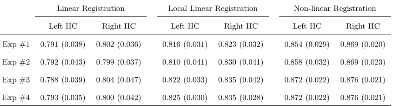
As mentioned in Sec. 2.3, the final segmented shape is the weighted combination of eigen-shapes derived from the training data. Therefore, the quality of the alignment (registration) between shapes might directly affect the segmentation accuracy. To study the effect of the different registration techniques on segmentation performance, we created three datasets each of which included the same 80 subjects, but were aligned using different registration methods: 1) linear registration, 2) local linear registration, and 3) non-linear registration. In each dataset, the 80 subjects were divided into four groups, each with 20 subjects. For each dataset, four experiments were conducted, and each experiment used one group of data as test subjects and used the remaining three groups of data as the training data. From the MR T1, T2/PD-images, both left and right of HC and AG are automatically identified and compared with manual labeling. The segmentation performance in terms of κ values based on the above three datasets is shown in Table 3 for HC segmentation, and Table 4 for AG segmentation. From these experiments, we can see:
Table 3: κ statistical result of HC segmentation
Linear Registration Local Linear Registration Non-linear Registration
Left HC Right HC Left HC Right HC Left HC Right HC
Exp #1 0.791 (0.038) 0.802 (0.036) 0.816 (0.031) 0.823 (0.032) 0.854 (0.029) 0.869 (0.020) Exp #2 0.792 (0.043) 0.799 (0.037) 0.810 (0.041) 0.830 (0.041) 0.858 (0.032) 0.869 (0.023) Exp #3 0.788 (0.039) 0.804 (0.047) 0.822 (0.033) 0.835 (0.042) 0.872 (0.022) 0.876 (0.021) Exp #4 0.793 (0.035) 0.800 (0.042) 0.825 (0.030) 0.835 (0.028) 0.872 (0.022) 0.876 (0.021) Values are mean κ and the standard deviations are in parentheses.
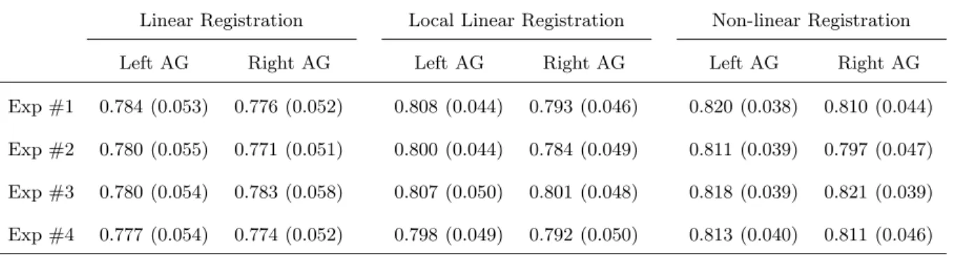
• In the HC segmentation, the individual κ values for the 80 subjects vary from 0.712 to 0.859 for the linearly registered data, 0.724 to 0.869 for linearly local registered data, and 0.754 to 0.907 for non-linearly registered data. The mean κ of the HC segmentation is 0.791 for left HC and 0.801 for right HC based on linearly registered data, 0.821 for left HC and 0.830 for right HC based on linearly local registered data, and 0.862 for left HC and 0.872 for right HC based on non-linearly registered data. In the AG segmentation, the individual κ values for the 80 subjects vary from 0.656 to 0.855 for the linearly registered data, 0.685 to 0.869 for linearly local registered data, and 0.695 to 0.879 for non-linearly registered data. The mean κ of the AG segmentation is 0.781 for left AG and 0.776 for right AG based on linearly registered data, 0.803 for left AG and 0.792 for right AG based on linearly local registered data, and 0.815 for left AG and 0.807 for right AG based on non-linearly registered data.
• In both HC and AG segmentation, for most subjects, the κ value from the non-linearly registered dataset is higher than those from the linearly local registered dataset and linearly registered dataset; while the κ value from the linearly local registered dataset is higher than one from linearly registered dataset. The mixed factors model repeated measure analysis (MFMRMA) using Manova (Cochran and Cox, 1957) shows a statistically significant effect on κ for the above three datasets (p ≤ 0.001). This statistical result indicates that the better alignment of the structure of interest among the datasets can significantly improve the segmentation accuracy in terms of κ.
To further evaluate the segmentation performance, in addition to κ, the similarity between the automatic result and manual labeling are also estimated by a volumetric comparison. The volumetric comparison uses linear regression to capture the volume differences between the automatic results and manual segmentations. The average volumes of the automatic results based on the variable weight
Table 4: κ statistical result of AG segmentation
Linear Registration Local Linear Registration Non-linear Registration
Left AG Right AG Left AG Right AG Left AG Right AG
Exp #1 0.784 (0.053) 0.776 (0.052) 0.808 (0.044) 0.793 (0.046) 0.820 (0.038) 0.810 (0.044) Exp #2 0.780 (0.055) 0.771 (0.051) 0.800 (0.044) 0.784 (0.049) 0.811 (0.039) 0.797 (0.047) Exp #3 0.780 (0.054) 0.783 (0.058) 0.807 (0.050) 0.801 (0.048) 0.818 (0.039) 0.821 (0.039) Exp #4 0.777 (0.054) 0.774 (0.052) 0.798 (0.049) 0.792 (0.050) 0.813 (0.040) 0.811 (0.046) Values are mean κ and the standard deviations are in parentheses.
Table 5: Statistical analysis of HC volume.
Manual labeling Automatic labeling Left HC Right HC Left HC Right HC Mean 4080 4319 4132 4372
Std Dev 487 415 483 403
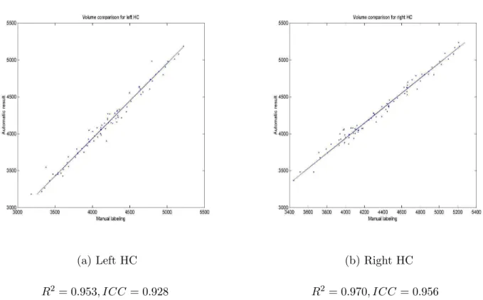
multi-contrast inputs method using non-linearly registered dataset and manual labels are shown in Table 5 for the HC and Table 6 for the AG. The volumetric comparison results between these two labellings are shown in Fig. 6 for the HC segmentation, and Fig. 7 for the AG segmentation. From those results, we can see:
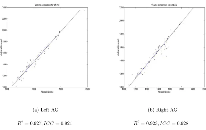
• For both HC and AG segmentation, automatically segmented HC and AG are slightly bigger than manual counterparts, but the difference is not statistically significant (p = 0.445 for HC and p = 0.185 for AG). Moreover, the agreement between two labellings in volume is very good since R2 and ICC values are high: above 0.9 for HC and AG.
• Both automatic results and manual labellings show that the volumes of the right HC are signifi-cantly bigger than that of the left HC (p ≤ 0.001). Since κ is sensitive to the structure size, this might explain why κ values of the right HC (around 0.873) are significantly higher than that of the left HC (around 0.864).
5
Discussion and Conclusions
In this paper, we present novel extensions to the level-set appearance-based method of structure segmentation by 1) integrating image data from multiple contrasts and 2) improving the
optimiza-Table 6: Statistical analysis of AG volume.
Manual labeling Automatic labeling Left AG Right AG Left AG Right AG Mean 1485 1472 1534 1520 Std Dev 242 230 233 224 (a) Left HC R2 = 0.953, ICC = 0.928 (b) Right HC R2 = 0.970, ICC = 0.956
Figure 6: Volumetric comparison between automatic results and manual labellings for HC segmenta-tions.
(a) Left AG
R2 = 0.927, ICC = 0.921
(b) Right AG
R2 = 0.923, ICC = 0.928
Figure 7: Volumetric comparison between automatic results and manual labellings for AG segmenta-tions.
tion algorithm used to synthesize new images. When tested on real MR images in the application of hippocampi and amygdalae segmentation, these modifications improve segmentation results over the basic single-image appearance-segmentation based method. Furthermore, the experimental re-sults have demonstrated feasibility, good performance, and robustness of this algorithm in 3D image segmentation.
In the experiments, we tested the proposed method using ICBM data set with 80 young healthy subjects. The four-fold cross validation experiments were conducted and each one had 60 training sub-jects and 20 testing subsub-jects. The experimental results of the 80 subsub-jects in 3D volumes demonstrated the segmentation accuracy (the mean κ of 0.87 with an ICC equal to 0.946 for the HC segmentation, and mean κ of 0.81 with an ICC equal to 0.924 for the AG segmentation), using the appearance model built on the training data with 60 subjects. Although the non-linear registration increases the computation time slightly, this additional computational investment significantly improves the segmentation results. With its relatively homogeneous young adult population, one issue related to the use of the ICBM database is perhaps its limited variability in shape and size of the HC and AG. While hippocampal volumes range from 2.2cc to 4.2cc in the ICBM cohort, one would expect greater variability in unhealthy cohorts such as patients with temporal lobe epilepsy, Alzheimers disease or
other neuro-degenerative disorder. Since the procedure is driven by the shape/appearance model built from the ICBM data, it may not be able to generate the smaller HC of patients with severe atrophy. While this may be a drawback for the current implementation, the method remains valid. In future work, we will add patient data to the training set, and apply procedure to MRI data of patients.
As demonstrated in the experimental results, the use of complementary information (such as T1, T2, and PD weighted MRI data) did improve the segmentation performance. In this context, we think the segmentation performance may be further improved by incorporating with tissue classification to remove CSF voxels. Furthermore, the experimental results demonstrated that the better alignment among the structures of interest improved the segmentation accuracy for the proposed appearance model-based segmentation method.
The proposed method was able to quickly segment a new subject. This is a significant advantage over other techniques (Collins and Pruessner, 2010) . Once aligned (6 minutes per subject for non-linear registration), only 3 minutes are required to process training data of 60 subjects in 3D with the size of 100 × 80 × 40 voxels to cover the volume of interest. The segmentation of a new subject requires 6 minutes (including non-linear registration) on a 1.5GHz Linux PC. This is roughly 10 times faster than the label fusion procedure proposed by Collins and Pruessner (Collins and Pruessner, 2010), while yielding almost the same accuracy.
Compared with many other techniques for the HC segmentation in the literature, the proposed method can provide comparable or somewhat better performance. However, due to the different anatomic definitions of the HC, different types of input data, and different qualities of manual seg-mentations, direct comparisons between different algorithms for HC segmentation might not be fair. Taking these caveats into consideration, we can compare our technique to the results of previous pub-lications. For example, Duchesne et al reported a mean of 0.650 for the left HC and 0.695 for the right HC (Duchesne et al., 2002). Klemencic et al (Klemencic et al., 2004) used the same method as Duch-esne et al but with a different registration technique to obtain κ ≈ 0.8 for the right HC segmentation. Also, Fischl et al in (Fischl et al., 2002) used the FreeSurfer method to demonstrate the overlap ratio (same as κ value) of 0.8, and the semi-automatic method developed by Hogan in (Hogan et al., 2000) showed the overlap ratio 0.83 for normal subjects and 0.66 for patients with atrophy. Other semi-automatic methods (Shen et al., 2002) showed good agreement between the algorithm and manual segmentations with a correlation coefficient equal to 0.97. Tu used the LONIBrainParser method to obtain a mean κ of 0.73 for the left HC and 0.63 for the right HC (Tu et al., 2008). For hippocampus segmentation in Alzheimer’s Disease and Mild Cognitive Impairment, κ values were less than 0.6 as
shown in (Carmichael et al., 2005). This result is probably due to the sensitivity of kappa to structure size combined with smaller hippocampi in the patient population. Recently, a number of new methods have been published. Aljabar et al in (Aljabar et al., 2009) developed multi-atlas based method and achieved a mean Dice overlap (same as κ) of 0.84 for HC segmentation. Collins and Pruessner (Collins and Pruessner, 2010) proposed a label fusion technique with template warping to yield a mean κ of 0.886. A similar mean κ (0.884) was reported by Coup´e et al. in (Coup´e et al., 2010) using a novel patch-based segmentation method evaluated on the same data. Patenaude in (Patenaude et al., 2011) used FIRST to achieve mean kappa of 0.81 for HC. The method proposed in this paper were also evaluated using the same data as (Collins and Pruessner, 2010; Coup´e et al., 2010), and the results achieved κ ≈ 0.87 and an ICC equal to 0.946 for normal subjects, indicating that our method can provide comparable segmentation performance in terms of accuracy and robustness with a significant improvement in speed compared to (Collins and Pruessner, 2010).
While a number of protocols exist for the manual segmentation of the amygdala (Pruessner et al., 2000, Bonilha et al., 2004), we can aware of only several other published methods on automatic segmentation of the amygdala. Except for HC, Fischl et al. in (Fischl et al., 2002) also reported overlap ratios of 0.75 for left AG and 0.78 for right AG. Heckemann et al (Heckemann et al., 2006) reported a similarity index (SI) (same as κ value) of 0.80 for the amygdala using a registration-based segmentation technique with an amygdala atlas. They also obtained a similarity index of 0.83 for HC. More recently, for AG segmentation, Aljabar et al (Aljabar et al., 2009) obtained a mean κ of 0.78, Collins and Pruessner (Collins and Pruessner, 2010) reported a mean κ 0.826, and Patenaude et al. (Patenaude et al., 2011) achieved a mean kappa of 0.74. In this paper, our method yielded κ ≈ 0.81 with the ICC equal to 0.924 for AG.
In conclusion, we have presented an automatic method of segmentation of the hippocampus and amygdala from normal subjects that takes advantage of complementary information from multiple con-trast images and the optimization procedures. Also, it is worthy to note that this proposed technique is a general segmentation method, and can be used to segment any structures whose configuration is roughly aligned, such as ventricles, and many blob-like central structures (e.g. caudate, and putamen) in addition to the HC and AG presented here. The experiments demonstrate that the use of multi-contrast images improves segmentation performance over using a single multi-contrast image. In addition, the experiments demonstrate the superiority of the variable weight multi-contrast input optimization procedure over our previous method. Taken together, the current results are encouraging in showing segmentation performance that ranks among the best seen in the literature. Future studies in clinical
populations will have to demonstrate if the small reduction in quality when compared to manual seg-mentation still allows to retrieve meaningful clinical information aimed at helping clinical diagnosis or monitoring treatment progress. If so, the current approach could allow to be introduced into clinical trials at little cost with the advantage over manual segmentation methods to be rater-independent and completely automated.
References
Aljabar, P., Heckemann, R., Hammers, A., Hajnal, J., and Rueckert, D. (2009). Multi-atlas based segmentation of brain iimages: Atlas selection and its effect on accuracy. NeuroImage, 46:726–738.
Bonilha, L., Kobayashi, E., Cendes, F., and Li, L. M. (2004). Protocol for volumetric segmentation of medial temporal structures using high-resolution 3-D magnetic resonance imaging. Human Brain Mapping, 22:145–154.
Borgefors, G. (1991). Another comment on a note on ’distance transformation in digital images’. In CVGIP-Image Understanding, volume 54, pages 301–306.
Carmichael, O., Aizenstein, H. J., Davis, S. W., Becker, J. T., Thompson, P. M., Meltzer, C. C., and Liu, Y. (2005). Atlas-based hippocampus segmentation in Alzheimer’s disease and mild cognitive impairment. NeuroImage, 27:979–990.
Cochran, W. C. and Cox, G. M. (1957). Experimental designs. 2nd Edition. New York: John Wiley
& Sons.
Collins, D., Neelin, P., Peters, T., and Evans, A. (1994). Automatic 3D intersubject registration of MR volumetric data in standardized Talairach space. J. of Comput. Assist. Tomogr., 18(2):192–205.
Collins, D. L. and Evans, A. C. (1997). Animal: Validation and applications of nonlinear registration-based segmentation. Int. J. Pattern Recognit. Artif. Intell., 11(8):1271–1294.
Collins, D. L. and Pruessner, J. C. (2010). Towards accurate, automatic segmentation of the hip-pocampus and amygdala from mri by augmenting animal with a template library and label. NeuroImage, 52:1355–1366.
Cootes, T., Edward, G., and Taylor, C. (1998). Active appearance model. In Proc. European Conf. Computer Vision, volume 2, pages 484–498.
Cootes, T. F. and Taylor, C. J. (2001). Statistical models of appearance for computer vision. Technical report, University of Manchester, Wolfson Image Analysis Unit, Imaging Science and Biomedical Engineering, Manchester M13 9PT, United Kingdom. Electronic version: http://www.isbe.man.ac.uk/∼bim/ref.html.
Coup´e, P., Manjon, J. V., Fonov, V., Pruessner, J., Robles, M., and Collins, D. L. (2010). Patch-based segmentation using expert priors: Application to hippocampus and ventricle segmentation. NeuroImage, (In press).
Davies, R. H. (2002). Learning shape: optimal models for analysing shape variability. PhD thesis, Division of Imaging Science and Biomedical Engineering, University of Manchester.
Dice, L. (1945). Measures of the amount of ecological association between species. Ecology, 26(3):297– 302.
Duchesne, S., Pruessner, J. C., and Collins, D. L. (2002). Appearance-based segmentation of medial temporal lobe structures. NeuroImage, 17:515–531.
Duzel, E., Schiltz, K., Solbach, T., Peschel, T., Baldeweg, T., Kaufmann, J., Szentkuti, A., and Heinze, H. J. (2005). Hippocampal atrophy in temporal lobe epilepsy is correlated with limbic systems atrophy. Journal of Neurology, 253(3):294–300.
Fischl, B., Salat, D. H., Busa, E., Albert, M., Dieterich, M., Haselgrove, C., van der Kouwe, A., Killiany, R., Kennedy, D., Klaveness, S., Montillo, A., Makris, N., Rosen, B., and Dale, A. M. (2002). Whole brain segmentation: automated labeling of neuroanatomical structures in the human brain. Neuron, 33:341–355.
Fonov, V. S., Evans, A. C., K. Botteron, C. R. A., McKinstry, R. C., Collins, D. L., and BDCG (2011). Unbiased average age-appropriate atlases for pediatric studies. NeuroImage, 54(1):313–327.
Fonov, V. S., Evans, A. C., McKinstry, R. C., Almli, C. R., and Collins, D. L. (2009). Unbiased nonlin-ear average age-appropriate brain templates from birth to adulthood. NeuroImage, 47(Supplement 1):S102–S102. Organization for human brain mapping 2009 annual meeting.
Gerig, G., Jomier, M., and Chakos, M. (2001). Valmet: A new validation tool for assessing and improving 3D object segmentation. Lecture Notes in Computer Science, 2208:516–523.
German, S. and McClure, D. (1987). Statistical methods for tomographic image reconstruction. Bulletin of the International Statistical Institute, 2:4–5.
Hechemann, R., Hajinal, J., Aljabar, P., Rueckert, D., and Hammers, S. (2006). Automatic anatomical brain mri segmentation combining label propagation and decision fusion. NeuroImage, 33(1):115– 126.
Heckemann, R. A., Hajnal, J. V., Aljabar, P., Rueckert, D., and Hammers, A. (2006). Automatic anatomical brain MRI segmentation combining label propagation and decision fusion. Neuroim-age, 33:115–126.
Hogan, R. E., Mark, K. E., Choudhuri, I., Wang, L., Joshi, S., Miller, M. I., and Bucholz, R. D. (2000). Magnetic resonance imaging deformation-based segmentation of the hippocampus in patients with mesial temporal sclerosis and temporal lobe epilepsy. J. Digit Imaging, 13:217–218.
Hu, S. and Collins, D. L. (2007). Joint level set shape modeling and appearance modeling for brain structure segmentation. NeuroImage, 36:672–683.
Kamber, M., Shinghal, R., Collins, D. L., Francis, G., and Evans, A. C. (1995). Model-based 3D segmentation of multiple sclerosis lesions in magnetic resonance brain images. IEEE Trans. Med. Imag., 14(3):442–453.
Klemencic, J., Pluim, J., Viergever, M., Schnack, H., and Valencic, V. (2004). Non-rigid registration based active appearance models for 3D medical image segmentation. Journal of Imaging Science and Technology, 48(2):166–171.
Leventon, M., Grimson, E., and Faugeras, O. (2000). Statistical shape influence in geodesic active contours. Computer Vision and Pattern Recognition, 1:316–323.
Mazziotta, J., Toga, A., Evans, A., Fox, P., Lancaster, J., Zilles, K., Woods, R., Paus, T., Simpson, G., Pike, B., Holmes, C., Collins, L., Thompson, P., MacDonald, D., Iacoboni, M., Schormann, T., Amunts, K., Palomero-Gallagher, N., Geyer, S., Parsons, L., Narr, K., Kabani, N., Goualher, G. L., Boomsma, D., Cannon, T., Kawashima, R., and Mazoyer, B. (2001). A probabilistic atlas and reference system for the human brain: International consortium for brain mapping (ICBM). Philos Trans R Soc Lond B Biol Sci., 356:1293–1322.
temporal structures relate to memory impairment in Alzheimer’s disease: an MRI volumetric study. J. Neurol. Neurosurg. Psychiatry, 63:214–221.
Osher, S. and Sethian, J. (1988). Fronts propagation with curvature dependent speed: Algorithms based on Hamilton-Jacobi formulations. J. Comput. Phys., 79:12–49.
Pal, N. R. and Pal, S. K. (1993). A review in image segmentation techniques. Pattern Recognition, 26(9):1277–1294.
Patenaude, B., Smith, S. M., Kennedy, D. N., and Jenkinson, M. (2011). A bayesian model of shape and appearance for subcortical brain segmentation. NeuroImage, (In press).
Pruessner, J. C., Collins, D. L., Pruessner, M., and Evans, A. C. (2001). Age and gender predict volume decline in the anterior and posterior hippocampus in early adulthood. The Journal of Neuroscience, 21(1):194–200.
Pruessner, J. C., Li, L. M., Serles, W., Pressner, M., Collins, D. L., Kabani, N., Lupien, S., and Evans, A. C. (2000). Volumetry of hippocampus and amygdala with high-resolution MRI and three-dimensional analysis software: Minimizing the discrepancies between laboratories. Cerebral Cortex, 10:433–442.
Rousson, M. (2004). Segmentation Incorporating Different Cues and Curve Evolution on Smooth Manifolds. PhD thesis, INRIA of Sophia Antipolis, Odyss´ee lab. Electronic version: http://mikael.rousson.googlepages.com/home.
Shattuck, D., Mirza, M., Adisetiyo, V., Hojatkashani, C., Salamon, G., Narr, K., Poldrack, R., Bilder, R., and Toga, A. (2008). Construction of a 3D probabilistic atlas of human cortical structures. NeuroImage, 39(3):1064–1080.
Shen, D., Moffat, S., Resnick, S. M., and Davatzikos, C. (2002). Measuring size and shape of the hippocampus in MR images using a deformable shape model. Neuroimage, 15:422–434.
Shout, P. E. and Fleiss, J. L. (1979). Intraclass correlations: Uses in assessing tater reliability. Psycholl Bull, 86:420–428.
Sled, J., Zijdenbos, A., and Evans, A. (1998). A nonparametric method of automatic correction of intensity nonuniformity in MRI data. IEEE Trans. Med. Imag., 17(1):87–97.
Tsai, A., Yezzi, A., Wells, J. W., Tempany, C., Tucher, S., A. Fan, W. E. G., and Willsky, A. (2003). A shape-based approach to the segmentation of medical imagery using level sets. IEEE Trans. Med. Imag., 22(2):137–154.
Tu, Z., Narr, K. L., Dollar, P., Dinow, I., Thompson, P. M., and w. Toga, A. (2008). Brain anatomical structure segmentation by hybrid discriminative/generative models. IEEE Trans. Med. Imag., 27(4):495–508.
Wang, L., Miller, J. P., Gado, M. H., McKeel, D., Miller, M. I., Morris, J. C., and Csernansky, J. G. (2005). Hippocampal shape abnormalities in early AD: A replication study. Alzheimer’s & Dementia: The Journal of the Alzheimer’s Association, 1(1):52–53.
Yang, J. and Duncan, J. (2004). 3D image segmentation of deformable objects with joint shape-intensity prior models using level sets. Medical Image Analysis, 8:285–294.