HAL Id: hal-02189499
https://hal.laas.fr/hal-02189499
Submitted on 19 Jul 2019
HAL is a multi-disciplinary open access
archive for the deposit and dissemination of
sci-entific research documents, whether they are
pub-lished or not. The documents may come from
teaching and research institutions in France or
abroad, or from public or private research centers.
L’archive ouverte pluridisciplinaire HAL, est
destinée au dépôt et à la diffusion de documents
scientifiques de niveau recherche, publiés ou non,
émanant des établissements d’enseignement et de
recherche français ou étrangers, des laboratoires
publics ou privés.
Flotation Process Fault Diagnosis Via Structural
Analysis
Carlos Gustavo Pérez Zuniga, J Sotomayor-Moriano, Elodie Chanthery,
Louise Travé-Massuyès, M. Soto
To cite this version:
Carlos Gustavo Pérez Zuniga, J Sotomayor-Moriano, Elodie Chanthery, Louise Travé-Massuyès, M.
Soto. Flotation Process Fault Diagnosis Via Structural Analysis. 18th IFAC Symposium on Control,
Optimization and Automation in Mining, Mineral and Metal Processing (MMM 2019), Aug 2019,
Stellenbosch, South Africa. �hal-02189499�
Flotation Process Fault Diagnosis Via
Structural Analysis
C. G. P´erez-Zu˜niga∗,∗∗ J. Sotomayor-Moriano∗ E. Chanthery∗∗ L. Trav´e-Massuy`es∗∗ M. Soto∗ ∗Engineering Department, Pontifical Catholic University of Peru,
PUCP (e-mail: [email protected], [email protected], [email protected])
∗∗LAAS-CNRS, Universit´e de Toulouse, CNRS, INSA, Toulouse,
France (e-mail: [email protected], [email protected]).
Abstract: For the improvement of safety and efficiency, fault diagnosis becomes increasingly important in mining industry. The expansion of flotation processes with high-tonnage cooper concentrators demands the use of large flotation circuits in which the large amount of instrumentation and interconnected subsystems (with coupled measured and non-measured variables) makes this process complex. Moreover, in a flotation process, any equipment failure can lead to a fault condition, which will affect the operation of this process. This paper proposes an approach for on-line fault diagnosis useful for a large flotation circuit based on a distributed architecture. In this approach, structural analysis is used for the design of the distributed fault diagnosis system. Finally, a procedure for the implementation of local diagnosers for on-line operation is presented and illustrated with an application to a flotation process.
Keywords: Fault diagnosis, Flotation process, Distributed architecture, Structural analysis 1. INTRODUCTION
Nowadays, the recovery is one of the most important process in mining industry. Currently, the recovery of minerals in this industry is mainly made through the flotation processing technique around the world.
Froth flotation uses the difference in surface properties to physically separate minerals from gangue and is one of the most widely used methods of ore concentration. In order to improve the recovery of valuable minerals, industrial flotation practice uses multiple cells. These cells are arranged in series forming a bank. A combination of banks is referred as flotation circuit. It is common for conventional flotation cells to be assembled in a circuit, with rougher, cleaner, and scavenger cells, which can be arranged in a designed configuration. On the other hand, in recent decades, the expansion of flotation with high-tonnage copper concentrators in Peru, Chile, etc. (O’Connell et al., 2016), has been demanding the use of large flotation circuits consisting of a large number of banks, with several cells each one.
Flotation equipment requires a machine for mixing and dispersing air throughout the mineral slurry while remov-ing the froth product. Instrumentation is also necessary for a successful implementation of control strategies. The ulti-mate aim of control is to increase the economic efficiency of the process by seeking to optimise performance, and there are several strategies which can be adopted to achieve this, (Wills, 2006). In the flotation process, any equipment fail-ure (in valves, sensors, pipelines, etc.), can lead to a fault condition, which will affect the operation of this process. In (Xu et al., 2012; Ming et al., 2015), methodologies for fault
detection in flotation process operation that use analysis of variables measurement are proposed. The use of Principal Component Analysis (PCA) models is proposed in (Bergh and Acosta, 2009) to detect instrumentation failures on a flotation column. The development of fault diagnosis systems in mining industry is very important because an effective diagnosis of faults may have a high economic and safety impact. However, fault diagnosis in large flota-tion circuits is a difficult task due not only to the large amount of instrumentation, but also to its interconnected subsystems with coupled (measured and non-measured) variables between them. In this case, the implementation of a global diagnoser may be an impractical option because of the amount of needed communication, (Blanke et al., 2016). Thus the use of centralized architecture for on-line fault diagnosis can be very expensive and lack robustness for large-scale interconnected subsystems, (P´erez-Zuniga et al., 2018). One possibility to overcome this difficulty is to employ a distributed diagnosis architecture.
Recently, a distributed diagnosis framework for physical systems with continuous behavior using structural model has been proposed in (Bregon et al., 2014) and a dis-tributed diagnosis approach with a set of diagnosers that are as local as possible was presented in (Khorasgani et al., 2015). In distributed diagnostic architectures, unlike centralized ones, it is not mandatory to know the model of the global system. Distributed architectures use subsystem models for diagnosis and local diagnosers (LDs), so they would be more appropriate for complex systems, (P´ erez-Zuniga et al., 2017), such as the large flotation circuits. The aim of this paper is to propose an approach for on-line fault diagnosis in flotation process circuit based on a
distributed architecture propose in (P´erez-Zuniga et al., 2017). In this approach, structural analysis is used as an efficient tool for the design of fault diagnosis systems for nonlinear processes, (Isermann, 2006). Likewise, in order to optimize the offline design of LDs, Fault-Driven Minimal Structurally Overdetermined (FMSO) sets are calculated and guarantee minimal redundancy of analytical redun-dancy relations (ARR) generators, (P´erez-Zuniga et al., 2015). At last, a procedure for the residual generation for on-line operation is presented and shown with the flotation process.
2. PROBLEM STATEMENT
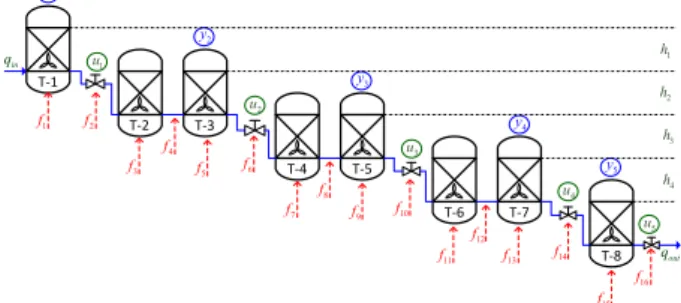
In a flotation process, the pulp is introduced into the first cell, the froth is collected through launders and the remaining pulp flows to the next cell. The magnitude of the flow depends on the pressure difference between two adjacent cells, the position of the control valves, and the viscosity and density of the pulp. Figure 1 shows the flotation process under study.
T-1 T-2 T-3 T-8 T-4 T-5 T-6 T-7 2 y 1 y 3 y 4 y 5 y 1 u 2 u 3 u 4 u 5 u in q h1 2 h 3 h 4 h 1 f f2 3 f 4 f 5 f f6 7 f 8 f 9 f f10 11 f 12 f 13 f f14 15 f 16 f out q
Fig. 1. Diagram of the flotation process under study. Due to the physical characteristics of the flotation process, and considering the disturbances caused by the composi-tion of the minerals and the constant and arduous work of the system, these systems usually have a limited efficiency, which is evidenced by faults in sensors, actuators and the system such as leaks in tanks and pipes, (Jamsa et al., 2003).
For the application of the structural analysis approach, let the system description consist of a set of n equations involving a set of variables partitioned into a set Z of nZ
known (or measured) variables and a set X of nXunknown
(or unmeasured) variables. We refer to the vector of known variables as z and the vector of unknown variables as x. The system may be impacted by the presence of nf faults
that appear as parameters in the equations. The set of faults is denoted by F and we refer to the vector of faults as f.
Definition 1. (System). A system, denoted Σ(z, x, f) or Σ for short, is any set of equations relating z, x and f. The equations ei(z, x) ⊆ Σ(z, x, f), i = 1, . . . , n, are assumed
to be differential or algebraic in z and x.
The flotation process under study has 5 levels at different altitudes (h1 to h5) and is composed of 41 equations (36
for the system and 5 linked to the level control of each stage). Later, we assumed each level with outlet pipe as a subsystem so this system is composed by 5 subsystems. The flow qinrefers to the pulp inflow, while the flow qoutis
related to the tailings. There are a set of 5 measurements y1 to y5 and a set of 5 control valves u1 to u5.
3. BACKGROUND THEORY
In this section, we summarize some important concepts presented in previous works related to the generation of diagnostic tests using structural analysis. Structural anal-ysis allows to obtain structural models that are very useful for the design of Model Based Diagnosis (MBD) systems. The main assumption is that each system component is described by one or several constraints; thereby, violation of at least one constraint indicates that the system com-ponent is faulty.
The structural model of the system Σ(z, x, f), also de-noted with some abuse of notation by Σ(z, x, f) or Σ in the following, can be obtained abstracting the functional equations. It retains a representation of which variables are involved in the equations. This abstraction leads to a bipartite graph G(Σ ∪ X ∪ Z, A), or equivalently to G(Σ ∪ X, A), where A ⊆ A and A is a set of edges such that a(i, j) ∈ A iff variable xi is involved in equation ej.
The structural model Σ(z, x, f) for this system is composed of 41 equations e1to e41relating the known variables Z =
{u1, u2, ..., u5, y1, y2, ..., y5, qin, qout}, the unknown
vari-ables X = { ˙x1, x1, ˙x2, x2, ˙x3, x3, ..., ˙x8, x8, q0, q1, q2, ..., q8}
and the set of sensors, actuators and process faults F = {f1, f2, f3, f4, f5, ..., f16}.
3.1 Analytical Redundancy Relations
Analytical redundancy relations (ARR) are equations that are deduced from an analytical model and only involve measured variables.
Definition 2. (ARR for Σ(z, x, f)). Let Σ(z, x, f) be a sys-tem. Then, a relation arr(z, ˙z, ¨z, ...) = 0 is an ARR for Σ(z, x, f) if for each z consistent with Σ(z, x, f) the rela-tion is fulfilled.
Definition 3. (Residual generator for Σ(z, x, f)). A system taking a subset of the variables z as input, and generating a scalar signal arr as output, is a residual generator for the model Σ(z, x, f) if, for all z consistent with Σ(z, x, f), it holds that lim
t→∞arr(t) = 0.
We use the decomposition of Dulmage Mendelshon as a tool to compute redundant sets using structural analysis, (Dulmage and Mendelsohn, 1958). Making use of this permutation, a system model Σ can be divided into three parts: the structurally overdetermined (SO) part Σ+ with more equations than unknown variables; the structurally just determined part Σ0, and the structurally underdeter-mined part Σ− with more unknown variables than equa-tions, (?).
Definition 4. (Structural redundancy). The structural re-dundancy ρΣ0 of a set of equations Σ0 ⊆ Σ is defined as the difference between the number of equations and the number of unknown variables in Σ0.
Definition 5. (Fault support). The fault support FΣ0 of a set of equations Σ0⊆ Σ is defined as the set of faults that are involved in the equations of Σ0.
Definition 6. (PSO and MSO sets). A set of equations Σ is proper structurally overdetermined (PSO) if Σ = Σ+
and minimally structurally overdetermined (MSO) if no proper subset of Σ is overdetermined (Krysander et al. (2010)).
Since PSO and MSO sets have more equations than vari-ables, they can be used to generate ARRs and residuals. A Fault-Driven Minimal Structurally Overdetermined (FMSO) set can be defined as an MSO set of Σ(z, x, f) whose fault support is not empty.
Let us define Zϕ ⊆ Z, Xϕ ⊆ X, and Fϕ ⊆ F as the
set of known variables, unknown variables involved in the FMSO set ϕ, and its fault support, respectively. Next, we summarize the definition of FMSO set,
Definition 7. (FMSO set). A subset of equations ϕ ⊆ Σ(z, x, f) is an FMSO set of Σ(z, x, f) if (1) Fϕ 6= ∅ and
ρϕ= 1 that means |ϕ| = |Xϕ| + 1, (2) no proper subset of
ϕ is overdeterminated. (P´erez-Zuniga et al., 2017) We propose the use of FMSO sets that guarantee to always be impacted to faults contrary to the MSO sets that not may not be impacted by faults. Based on the concept of FMSO set, we summarize the concept of detectable fault, and isolable fault :
Definition 8. (Detectable fault). A fault f ∈ F is de-tectable in the system Σ(z, x, f) if there is an FMSO set ϕ ∈ Φ such that f ∈ Fϕ.
Definition 9. (Isolable fault). Given two detectable faults fj and fk of F , j 6= k, fj is isolable from fk if there exists
an FMSO set ϕ ∈ Φ such that fj∈ Fϕ and fk 6∈ Fϕ.
Additionally, a Clear Minimal Structurally Overdeter-mined (CMSO) set is a MSO set of Σ(z, x, f) whose fault support is empty.
3.2 Distribution and Related Notions
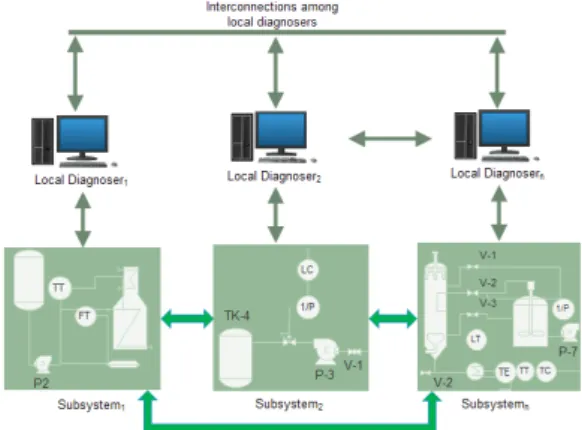
A distributed diagnosis architecture assumes a decompo-sition of the process into subsystems, each with its cor-responding LD, with similar functions and with possible communication between them. This communication must be properly designed; therefore, the local diagnoses are globally consistent. This architecture is shown in Figure 2.
Fig. 2. Distributed diagnosis architecture
For the flotation process, in this paper we propose the design of the distributed system taking into account only
the models of each subsystem to design LDs independently considering minimizing the communication between them until reaching the same diagnosis as with a centralized diagnosis. Let us consider the system Σ and define the following:
A decomposition of the system Σ(z, x, f), into several sub-systems Σi(zi, xi, fi) is defined as a partition of its
equa-tions. Let Σ(z, x, f) = {Σ1(z1, x1, f1), ..., Σn(zn, xn, fn)} with Σi(zi, xi, fi) ⊆ Σ(z, x, f), n S i=1 Σi(zi, xi, fi) = Σ, Σi(zi, xi, fi) 6= ∅ and Σi(zi, xi, fi) ∩ Σj(zj, xj, fj) = ∅
if i 6= j. where zi is the vector of known variables in
Σi, xi is the vector of unknown variables in Σi and fi
is the vector of faults in Σi. The set of variables and
faults of the ith subsystem Σi, denoted as Xi, Zi, and Fi
respectively, are defined as the subset of variables of X, Z, and F respectively, that are involved in the subsystem Σi(zi, xi, fi) also denoted by Σi.
For the flotation process, we consider each level as a subsystem, therefore, the first subsystem includes a tank and the outlet pipe, the second to the fourth subsystems, contain 2 tanks, the pipe between them and the outlet pipe and the fifth subsystem includes a tank and the outlet pipe, see Table 1.
Table 1. Model decomposition of the flotation process system into subsystems Σi(zi, xi, fi),
i = 1, 2, 3, 4, 5. Σ1= {e1, e2, e3, e4, e5, e6, e7} F1= {f1, f2} X1= { ˙x1, x1, q0, w1} Z1= {u1, y1, qin} Σ2= {e8, e9, e10, ..., e16} F2= {f3, f4, f5, f6} X2= { ˙x2, x3, ˙x3, q2, w2} Z2= {u2, y2} Σ3= {e17, e18, e19, ..., e25} F3= {f7, f8, f9, f10} X3= { ˙x4, x5, ˙x5, q4, w3} Z3= {u3, y3} Σ4= {e26, e27, e28, ..., e34} F4= {f11, f12, f13, f14} X4= { ˙x6, x7, ˙x7, q6, w4} Z4= {u4, y4} Σ5= {e35, e36, e37, ..., e40} F5= {f15, f16} X5= { ˙x8, q8, w5} Z5= {u5, y5}
The set of local variables of the ithsubsystem, denoted by Xl
i, is defined as the subset of variables of Xithat are only
involved in the subsystem Σi.
Definition 10. (Shared variables). The set of shared vari-ables of the ithsubsystem, denoted as Xs
i, is defined as: Xis= n [ j=1,j6=i (Xi∩ Xj) = Xi\ Xil (1)
The set of shared variables of the whole system Σ is denoted by Xs.
Without loss of generality, we consider that all known vari-ables of Zi are local to the subsystem Σi, for i = 1, . . . , n.
If the same input was applied to several subsystems, it could be artificially replicated.
3.3 Distributed FMSO sets
Definition 11. (Local FMSO set). ϕ is a local FMSO set of Σi(zi, xi, fi) if ϕ is an MFSO set of Σ(z, x, f) and if
ϕ ⊆ Σi, Xϕ ⊆ Xi and Zϕ ⊆ Zil. The set of local FMSO
sets of Σiis denoted by Φli. The set of all local FMSO sets
is denoted by Φl=
n
S
i=1
Φli.
Definition 12. (Shared FMSO set). ϕ is a shared FMSO set of subsystem Σi(zi, xi, fi) if ϕ is an FMSO set of
˜
Σi(˜zi, ˜xi, ˜fi), where ˜ziis the vector of variables in ˜Zi= Zi∪
Xs
i, ˜xiis the vector of variables in ˜Xi= Xil, and ˜fi= fi).
The set of shared FMSO sets for Σi is denoted by Φsi. The
set of all shared FMSO sets is denoted by Φs= Sn
i=1
Φs i.
From the above definition, a shared FMSO set ϕ for subsystem Σi(zi, xi, fi) is such that ϕ ⊆ Σi, Xϕ ⊆ Xil,
Zϕ∩ Xis6= ∅, and Zϕ⊆ (Zi∪ Xis).
Definitions 11 and 12 can also be applied to CMSO sets to define local CMSO sets Λli and shared CMSO sets Λsi. The set of all shared CMSO sets is denoted by Λs.
Definition 13. (Compound FMSO set). A global FMSO set ϕ that includes at least one shared FMSO set ϕ0 ∈ Φs
iis
called a compound FMSO set. The set of compound FMSO sets of Σiis denoted by Φci. The set of all compound FMSO
sets is denoted by Φc =
n
S
i=1
Φci.
Definition 14. (Root FMSO set). If a compound FMSO set ϕ ∈ Φc includes a shared FMSO set ϕ0 ∈ Φs, then
ϕ0 is a root FMSO set of ϕ.
Definition 15. (Locally detectable fault). f ∈ Fiis locally
detectable in the subsystem Σi(zi, xi, fi) if there is an
FMSO set ϕ ∈ Φl
i such that f ∈ Fϕ.
Definition 16. (Locally isolable fault). Given two locally detectable faults fj and fk of Fi, j 6= k, fj is locally
isolable from fk if there exists an FMSO set ϕ ∈ Φli such
that fj∈ Fϕ and fk 6∈ Fϕ.
Some properties required for the generation of compound FMSO sets starting from shared FMSO sets are detailed in P´erez-Zuniga et al. (2017)
4. DISTRIBUTED DIAGNOSIS
First, a set of distributed local diagnosers (LD) that together make the entire system completely diagnosable through compound FMSO sets is obtained, then residual generators that make it possible to detect and isolate all system faults are implemented. First, Algorithm 1 for generating local diagnostics off-line is applied and then Algorithm 2 is proposed for on-line residual generation. 4.1 Offline distributed generation of LDs
The LD design is done off-line in Algorithm 1. First, local FMSO sets are computed for every subsystem Σi.
If there is any fault not locally detectable, then a set of compound FMSO sets is calculated to achieve full diagnosability for all the faults in Fi. The procedure to
compute ’good’ compound FMSO sets starting with ϕ∗as a root FMSO set makes use of an optimization heuristic based on the number of shared variables and on the number of subsystems involved with the aim of minimizing communication between subsystems.
Algorithm 1. Offline Generation of LDs. 1: for i=1...n do
2: Φi = ∅;
3: Φl
i ← Calculate local FMSO sets of Σi;
4: if there is any fault f ∈ Fi not locally detectable
5: or not locally isolable with the set of local
6: FMSO sets Φli then
7: Φs
i ← Calculate shared FMSO sets of Σi;
8: Λsi ← Calculate shared CMSO sets of Σi;
9: end if
10: while it exists f ∈ Fi that is not detectable
11: or isolable do
12: Let ϕ∗∈ Φs
i such that f ∈ Fϕ∗ be the ’best’
13: (not already selected) shared FMSO set of Φsi;
14: Label ϕ∗ as root FMSO set: ϕr← ϕ∗;
15: Let Xϕsr be the set of shared variables of ϕr;
16: Φc∗
i ← Build a ’good’ compound FMSO set
17: including ϕ∗by always selecting the ’best’ 18: shared FMSO sets to cover newly introduced
19: shared variables;
20: Φi← Φi∪ Φc∗i ;
21: Φl∗
i ← Find a minimal cardinality set of local
22: FMSO sets achieving the same diagnosability
23: as all local FMSO sets;
24: Φi← Φi∪ Φl∗i ;
25: end while
26: end for
4.2 On-line distributed residual operation of LDs
After the off-line design of the LDs performed with algo-rithm 1, the online operation of the distributed diagnoser relies on the bank of residual generators ARRi selected
for each LD LDi, i = 1, . . . , n, fed by measured signals
from their corresponding subsystems. As shown in Figure 3, fault isolation is carried out after fault detection using local fault signature matrices according to Definition 17. Definition 17. (FSM of a subsystem). Given a set ARRi
composed of nr
i ARRs and Fi the set of considered n f i
faults for the subsystem Σi and consider the function
ARRi× Fj,i −→ 0, 1, then the signature of a fault f ∈
Fi is the binary vector F Si(f ) = [τ1, τ2, ...τnr i]
T where
τk = 1 if f is involved in the equations used to form
arrk ∈ ARRi, otherwise τk = 0. The signatures of all
the faults in Fi together constitute the fault signature
matrix (FSM) F SMi for subsystem Σi, i.e. F SMi =
[F Si(f1), . . . , F Si(fnf i
)]T.
5. APPLICATION TO THE FLOTATION PROCESS 5.1 Offline distributed generation of LDs
In this section, the construction of the LD for each sub-system is presented in order to diagnose all sub-system faults. Below the steps of the offline design:
1.- The local FMSOs are calculated for each of the sub-systems, considering only local information.
Φl1= Φl2= Φ3l = Φl4= Φl5= ∅ (2) No local FMSOs were found considering only informa-tion from each subsystem. The shared FMSOs for each
Fig. 3. Scheme of distributed generation of LDs.
Algorithm 2. On-line Residual Operation of LDs. 1: for i=1...n do
2: For each LD:
3: Compute ARRs for LDi
4: for j=1...m do
5: For all selected compound FMSO sets:
6: ARRi,j ← Compute analytical residual
7: generators of LDi;
8: Save the set of known variables of
9: each ARRj,i;
10: ZLDi← ZLDi∪ ZARRj,i;
11: end for
12: By means of the fault signature matrix (F SMi)
13: verify the isolability of faults of each subsystem;
14: end for
15: Add the known variables of the vector ZLDi to the fault diagnosis software for the online calculation of the ARRs of the LDs;
16: Generate a on-line scalar signal arrk from
17: the respective ARRj,iusing the signals of ZLDi . subsystem are then determined by considering the vector of shared variables (Xs= {x
2, x4, x6, x8, q1, q3, q5, q7}) as
part of the vector of known variables for each subsystem. 2.- For subsystems σ1 to σ5, shared FMSO sets are
computed, Results are given in Table 3.
3.- For each subsystem, Algorithm 1 chooses from the set of shared FMSO sets, a subset that is labeled as root FMSO set and complete with a shared FMSO set each of its shared variables until get a set of compound FMSO sets that can diagnose all the faults of that subsystem. The set of compound FMSO sets capable of detecting and isolating the faults constitute the LD of the corresponding subsystem. Results are given in Table 3.
5.2 On-line distributed residual operation of LDs
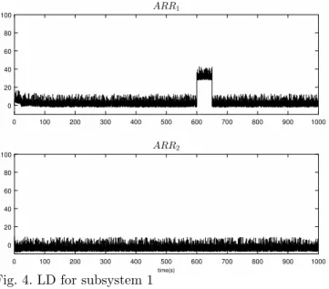
Using Algorithm 2, the ARRs are calculated and the isolation of the 16 faults of this system is verified, as shown in Table 4 to 8. As example, Figure 4 shows the ARRs operating online for subsystem 1, as can be seen in the case of a momentary fault of the tank level sensor 1 (f1)
from 600 s. up to 650 s., there is a detection of ARR1and
no detection of ARR2, which demonstrates the isolation
of this fault locally.
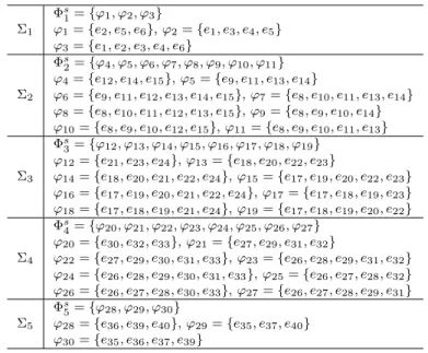
Φs1= {ϕ1, ϕ2, ϕ3} Σ1 ϕ1= {e2, e5, e6}, ϕ2= {e1, e3, e4, e5} ϕ3= {e1, e2, e3, e4, e6} Φs2= {ϕ4, ϕ5, ϕ6, ϕ7, ϕ8, ϕ9, ϕ10, ϕ11} ϕ4= {e12, e14, e15}, ϕ5= {e9, e11, e13, e14} Σ2 ϕ6= {e9, e11, e12, e13, e14, e15}, ϕ7= {e8, e10, e11, e13, e14} ϕ8= {e8, e10, e11, e12, e13, e15}, ϕ9= {e8, e9, e10, e14} ϕ10= {e8, e9, e10, e12, e15}, ϕ11= {e8, e9, e10, e11, e13} Φs 3= {ϕ12, ϕ13, ϕ14, ϕ15, ϕ16, ϕ17, ϕ18, ϕ19} ϕ12= {e21, e23, e24}, ϕ13= {e18, e20, e22, e23} Σ3 ϕ14= {e18, e20, e21, e22, e24}, ϕ15= {e17, e19, e20, e22, e23} ϕ16= {e17, e19, e20, e21, e22, e24}, ϕ17= {e17, e18, e19, e23} ϕ18= {e17, e18, e19, e21, e24}, ϕ19= {e17, e18, e19, e20, e22} Φs 4= {ϕ20, ϕ21, ϕ22, ϕ23, ϕ24, ϕ25, ϕ26, ϕ27} ϕ20= {e30, e32, e33}, ϕ21= {e27, e29, e31, e32} Σ4 ϕ22= {e27, e29, e30, e31, e33}, ϕ23= {e26, e28, e29, e31, e32} ϕ24= {e26, e28, e29, e30, e31, e33}, ϕ25= {e26, e27, e28, e32} ϕ26= {e26, e27, e28, e30, e33}, ϕ27= {e26, e27, e28, e29, e31} Φs 5= {ϕ28, ϕ29, ϕ30} Σ5 ϕ28= {e36, e39, e40}, ϕ29= {e35, e37, e40} ϕ30= {e35, e36, e37, e39}
Table 2. Shared FMSO sets of Σ1to Σ5.
LD1 ϕ31= {e1, e2, e3, e4, e5, e6, e8, e9, e10, e14} ϕ32= {e2, e5, e6, e8, e9, e10, ..., e15, e17, e18, e19, e23} LD2 ϕ33= {e1, ..., e6, e9e11e13, e17, ..., e24, e26, e27, e28, e32} ϕ34= {e1, ..., e6, e8, e10, e11, e13, e14e17, ..., e22, e23, e24, e26, e27, e28, e32} LD3 ϕ35= {e2, e5, e6, e8, ..., e15, e18, e20, e22, e23, e26, ..., e33, e38} ϕ36= {e2, e5, e6, e8, ..., e15, e17, e19, e20, e22, e23, e26, ..., e33, e38} LD4 ϕ37= {e12, e14, e15, e17, ..., e24, e27, e29, e31, e32, e35, e37, e38, e40} ϕ38= {e12, e14, e15, e17, ..., e24, e26, e28, e29, e31, e32, e35, e37, e38, e40} LD5 ϕ39= {e30, e32, e33, e35, e37, e38, e40} ϕ40= {e36, e38, e39, e40}
Table 3. Compound FMSO sets of LDs.
Faults
f1 f2
arr1∈ ARR1,1 X
arr2∈ ARR1,2 X
Table 4. isolation capability for ARRs for LD1.
Faults
f3 f4 f5 f6
arr3∈ ARR2,1 X X
arr4∈ ARR2,2 X X
Table 5. isolation capability for ARRs for LD2.
Faults
f7 f8 f9 f10
arr5∈ ARR3,1 X X
arr6∈ ARR3,2 X X
Table 6. isolation capability for ARRs for LD3.
Finally, Figure 5 shows the human machine interface of the fault diagnosis software running on-line where a fault alarm is shown in valve 2 (f6). This software is executed
Faults
f11 f12 f13 f14
arr7∈ ARR4,1 X X
arr8∈ ARR4,2 X X
Table 7. isolation capability for ARRs for LD4.
Faults
f15 f16
arr9∈ ARR5,1 X
arr10∈ ARR5,2 X
Table 8. isolation capability for ARRs for LD5.
0 100 200 300 400 500 600 700 800 900 1000 0 20 40 60 80 100 ARR 1 time(s) 0 100 200 300 400 500 600 700 800 900 1000 0 20 40 60 80 100 ARR2
Fig. 4. LD for subsystem 1
in a programmable automation controller (PAC) that receives the signals from the sensors and generates the control signals.
Fig. 5. Fault diagnosis software
In fact, the proposed approach is applicable to fault diagnosis of a large floating circuit, decomposing the latter into subsystems. Here, as shown above, each subsystem in the distributed architecture will have its own LD.
6. CONCLUSION
An approach for on-line fault diagnosis in a flotation process was proposed based on a distributed architecture. The application of the approach allows the development of diagnosis systems for large-scale flotation circuits. The fault diagnosis system developed, was tested by simulation
validating that the 16 faults can be detected and isolated locally or at a higher level. Likewise, a procedure for residual generation was presented and it has been tested into a programmable automation controller for on-line operation of fault diagnosis software.
7. AKNOWLEDGMENTS
This work was funded by Proyecto de Mejoramiento y Ampliaci´on de los Servicios del Sistema Nacional de Cien-cia Tecnolog´ıa e Innovaci´on Tecnol´ogica’ 8682-PE, Banco Mundial, CONCYTEC and FONDECYT through grant N48-2018-FONDECYT-BM-IADT-MU.
REFERENCES
Bergh, L. and Acosta, S. (2009). On-line fault detection on a pilot flotation column using linear pca models. Computer Aided Chemical Eng. vol. 27 pp. 1437-1442. Blanke, M., Kinnaert, M., Lunze, J., and Staroswiecki, M.
(2016). Diagnosis and Fault-Tolerant Control. Springer. Bregon, A., Daigle, M., Roychoudhury, I., Biswas, G., Koutsoukos, X., and Pulido, B. (2014). An event based distributed diagnosis framework using structural model decomposition. Art. Int. vol. 210 pp.1-35.
Dulmage, A.L. and Mendelsohn, N.S. (1958). Coverings of bipartite graphs. Canadian Journal of Mathematics, vol. 10, pp. 517-534.
Isermann, R. (2006). Fault-Diagnosis Systems. Springer-Verlag Berlin Heidelberg.
Jamsa, S., Dietrich, M., Halmevaara, K., and Tiili, O. (2003). Control of pulp levels flotation cells. Control Engineering Practice vol 11 pp. 73-81.
Khorasgani, H., Jung, D., and Biswas, G. (2015). Struc-tural approach for distributed fault detection and isola-tion. IFAC-PapersOnline Vol. 48 Issue 21 pp. 72-77. Krysander, M., Aslund, J., and Frisk, E. (2010). A
structural algorithm for finding testable sub-models and multiple fault isolability analysis. In 21st International Workshop on the Principles of Diagnosis.
Ming, L., Wei-hua, G., Tao, P., and Wei, C. (2015). Fault condition detection for a copper flotation process based on a wavelet multi-scale binary froth image. Rev. Esc. Minas vol. 68 no.2.
O’Connell, R., Alway, B., Sischka, B., Norton, K., Yao, W., Wong, L., Bakourou, V., and Salmon, B. (2016). Gfms copper survey 2016. Thomson Reuters.
P´erez-Zuniga, C., Chantery, E., Trav-Massuyes, L., So-tomayor, J., and Artigues, C. (2018). Decentralized di-agnosis via structural analysis and integer programming. IFAC-PapersOnline 51-24 pp. 168-175.
P´erez-Zuniga, C., Chanthery, E., Trav´e-Massuy`es, L., and Sotomayor-Moriano, J. (2017). Fault-driven structural diagnosis approach in a distributed context. In IFAC PapersOnline 50-1 14254-14259.
P´erez-Zuniga, C., Trav-Massuyes, L., Chantery, E., and Sotomayor, J. (2015). Decentralized diagnosis in a spacecraft attitude determination and control system. Journal of Physics: Conf Series vol. 659(1) pp. 1-12. Wills, B. (2006). Mineral Processing Technology.
Butterworth-Heinemann, Oxford, UK.
Xu, C., Gui, W., Yang, C., Zhu, H., Lin, Y., and Shi, C. (2012). Flotation process fault detection using output pdf of bubble size distribution. Minerals Engineering vol. 26 pp. 5-12.