Estimation of Local Mean Population Densities of Japanese Beetle
Grubs (Scarabaeidae: Coleoptera)
D. DALTHORP, J. NYROP,ANDM. VILLANI
Department of Entomology, Cornell University, NYSAES, Geneva, NY 14456
Environ. Entomol. 28(2): 255Ð265 (1999)
ABSTRACT Insect populations tend to be patchy in distribution. Even when the mean population density is low, there may be local patches with high densities. As a result, estimates of mean populations may provide little information about the size or intensity of local patches within the sampled area. We compared the following 3 methods of estimating local population densities of insects: (1) with moving averages, a local mean population density is estimated as the mean of samples taken within a given radius of a central point, (2) with inverse distances, local means are estimated as weighted averages of samples; each sample is given a weight proportional to a power of the reciprocal of its distance from the center of the region for which the mean is to be estimated, (3) krigingis a geostatistical algorithm for estimating local means as weighted averages of samples. Weighting is based on the spatial covariance of the samples, or the degree to which samples that are near to each other are related. The Þrst 2 methods are relatively easy to calculate but were unreliable when used with standard parameters to estimate local Japanese beetle grub densities. When an optimum radius was used with moving averages and an optimum exponent was used with inverse distances, the advantage of ease of calculation was lost, yet both methods were still inferior to kriging in providing accurate estimates of local means.
KEY WORDS Popillia japonica, larvae, spatial statistics, inverse distance, kriging, dispersion
INSECT POPULATION DENSITIESare commonly estimated
as the mean of a set of sample observations. This approach works well for estimating overall mean pop-ulations, but more sophisticated approaches to esti-mating local means are needed when identiÞcation of patches with high or low density is desired. Because the distribution of agricultural pests is often patchy, pest populations may be high enough in some parts of a Þeld to damage a crop, whereas other parts of the Þeld remain virtually pest-free (Nyrop et al. 1995; Weisz et al. 1995a, b). Targeting management tactics such as application of insecticides to the parts of the Þeld that harbor high pest populations may retard the development of resistance in the pest population and conserve natural enemies (e.g., Midgarden et al. 1997). Such precision management of insect pests re-quires reliable methods for estimating mean popula-tion densities in the smallest areas or blocks in which signiÞcant damage could occur. When a single sample observation provides a good estimate of mean density within a block surrounding the sample, or when many samples can be taken within the block so that a reliable estimate of the mean density can be made by taking the average of the observations, the problem of esti-mating the local means is solved. These solutions are not feasible when individual sample observations are poor estimators of the local population means, and it is not feasible to take several samples within each block. In such cases, it may still be possible to estimate local means reliably by taking advantage of spatial
autocorrelation, or the tendency of neighboring sam-ples to have similar values.
We were faced with this problem of estimating local means for larvae of Japanese beetle, Popillia japonica Newman, on golf course fairways. The fairways are mixed plantings of turfgrass, each covering 6,000Ð16,000 m2. Golf courses normally contain 18
fairways, or some 200,000 m2 of intensely managed
turf. In the eastern United States, Japanese beetle larvae are common pests on these plantings. Visible grub damage can occur in block of turf as little as 45Ð90m2. Given the highly variable distribution of
Jap-anese beetle larvae in these turf plantings, reliable estimates of local population densities could be useful management aids.
A golf course may contain .3, 000 blocks in which to estimate local means, so it may not be feasible to collect several samples in each block. In addition, the small size of each sample (0.008 m2) precludes it from
being a precise estimate of a local mean. We compared several methods of taking advantage of spatial covari-ance of population density to use information from nearby blocks to estimate the mean of a given block. Each method estimates a block mean as a weighted average of samples in and around the block. Weights decrease as a function of distance from the center of the block. The methods differ only in how those weights are assigned. The 3 methods of estimating local means were compared on the basis of effective-ness (or ability to make correct estimates) and stabil-0046-225X/99/0255Ð0265$02.00/0 q 1999 Entomological Society of America
ity (or ability to give consistent results), as discussed below.
Moving Averages. With the method of moving
erages, a local or block mean is estimated as the av-erage of all samples within a given radius of the center of the block. Moving averages has the advantage that local means are easy to calculate. Disadvantages of this method are that it is difÞcult to determine the most appropriate radius for smoothing, and the implicit model of spatial covariance may not be correct, in which case good estimates of local means would not be obtained.
Inverse Distances. Isaaks and Srivastava (1989)
pro-vide an excellent discussion of the commonly used inverse distance method for spatial interpolation and map generation. However, the method must be mod-iÞed if it is to be used for estimating local means. The modiÞed method is discussed below, and details of the modiÞcations are discussed in the Appendix 1.
Local means are estimated as weighted averages of the samples taken on a fairway. Weights assigned to sample points are proportional to a power of the in-verse of the distance from the sample to the center of the block. Points far from the block thus receive little weight, and points close to the block receive relatively high weights. The weights are normalized so that they sum to 1. The estimate of the block mean is the weighted average of all points on the fairway, viz.
mˆj5 wjzj1
O
iÞj 1 dipzi wj1O
iÞj 1 dip , [1]wheremˆ, is the estimate of the mean population den-sity in block j, diis the distance from the center of the
block to sample i, ziis the number of grubs observed
in sample i, and wjis the weight assigned to the sample
at the center of the block (see Appendix and Table 2). The gradual decline in weights with distance is intu-itively satisfying, yet the weights are still relatively easy to calculate. A priori disadvantages are that the implicit model of spatial covariance (or how the weights decline) is not very ßexible, and optimization of the exponent p requires considerable computation.
Block Kriging. With block kriging, local means are
again estimated as a weighted average of the samples (Isaaks and Srivastava 1989, Deutsch and Journel 1992). Weights are based on an explicit model of the spatial covariance of the data. We used the covario-gram to quantify the covariance (Cressie 1993, Kaluzny et al. 1996). For each fairway, 2 different covariance models were used: omnidirectional and directional. Omnidirectional models assume that the covariance is strictly a function of separation distance or lag. With directional models, covariance is modeled as a function of both the lag distance and direction. Directional models are useful when populations are more continuous in 1 direction than another, as com-monly occurs when an environmental gradient changes more rapidly in one direction than another. The advantage of this method is that the model of spatial covariance is explicit and ßexible, resulting in relatively reliable estimates of local means. The main disadvantage is that the method does require explicit modeling of the spatial covariance.
Comparison of the Methods. Effectiveness. The
ef-fectiveness of estimation methods can be quantiÞed Table 1. Summary of sample counts of Japanese beetle grubs on 2 golf courses for each of 2 yr
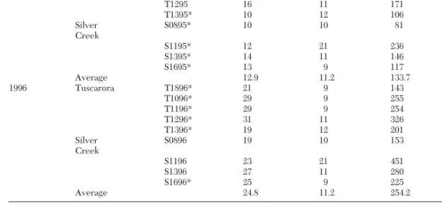
Year Golf course Fairway Rowsa Columnsb n Meanc Variance
1995 Tuscarora T1895 11 9 82 0.805 1.122 T1095 15 9 130 1.023 1.961 T1195* 15 9 134 1.709 3.546 T1295 16 11 171 1.047 2.621 T1395* 10 12 106 1.085 1.621 Silver Creek S0895* 10 10 81 1.062 2.734 S1195* 12 21 236 0.822 1.960 S1395* 14 11 146 1.356 3.169 S1695* 13 9 117 0.872 1.544 Average 12.9 11.2 133.7 1.087 2.253 1996 Tuscarora T1896* 21 9 143 0.664 1.239 T1096* 29 9 255 0.808 1.463 T1196* 29 9 254 1.280 2.732 T1296* 31 11 326 0.546 0.907 T1396* 19 12 201 0.866 1.327 Silver Creek S0896 19 10 153 0.275 0.398 S1196 23 21 451 0.188 0.291 S1396 27 11 280 0.154 0.166 S1696* 25 9 225 0.231 0.384 Average 24.8 11.2 254.2 0.557 0.990
Fairways for which detailed spatial analyses were performed are indicated by asterisks.
aNumber of rows of samples taken across fairway. bNumber of columns of samples taken along fairway. cAverage number of grubs per sample.
by comparing estimates to true values using cross-validation. In cross-validation, actual data points are dropped one at a time and reestimated from the re-maining data. Thus, the sample count at the center of a block is ignored when calculating the cross-valida-tion estimate for that block. Once a datum has been reestimated using an estimation method, it is put back into the data set and the procedure is repeated for the next datum (Deutsch and Journel 1992). In this way a cross-validation data set is constructed for each esti-mation method with 1 cross-validation estimate cor-responding to each point in the data set. Cross-vali-dation estimates are subtracted from the raw data values to obtain the validation errors. The cross-validation errors measure how well a given method estimates means at ÔunsampledÕ locations. Thus, an effective method should have relatively small cross-validation errors.
Stability. Stability of an estimation method is de-Þned in terms of the similarity of its interpretation of local means for different smoothing parameters (e.g., the radius for moving averages). Different smoothing parameter values result in unique topographical maps or surfaces of block means, with peaks of high density and valleys of low density. For example, with decreas-ing inverse distance exponent or increasdecreas-ing movdecreas-ing average radius, each estimated local mean approaches the overall sample mean, so the density surface be-comes smoother. Conversely, for large inverse dis-tance exponent or small moving average radius, the density surface is relatively rough.
With fortuitous circumstances in some applications, choice of a smoothing parameter within a wide range of values does not signiÞcantly affect the interpreta-tion of the data (e.g., Weisz et al. 1995a, b). In such situations, a carefully selected value may be chosen as a standard value for widespread use. However, in other situations the interpretation of data can change substantially with small changes in parameter values, making the estimation method unreliable if a standard smoothing parameter is used.
A stability index can be used to quantify the differ-ences in the topographies of density surfaces resulting from small changes in smoothing parameter values. This index then can be used as a relative measure of stablity to compare estimation methods for a single set of data. The stability index also can be used to deter-mine when instability precludes the use of a standard inverse distance exponent or moving average radius for a collection of data sets.
Materials and Methods
Sampling. Five fairways at Tuscarora Country Club
in Camillus, NY, and 4 at Silver Creek Country Club in Waterloo, NY, were sampled for 2nd and 3rd instars of Japanese beetle in late August and early September 1995 and 1996. The fairways were '200 m long and 40 m wide. All were irrigated, and normal applications of fertilizers, herbicides, and fungicides were applied
as needed. Insecticides were not applied in the spring or summer before each yearÕs sampling, but bendio-carb was applied to the Tuscarora fairways after sam-pling.
Circular soil cores 10 cm in diameter and '10 cm. deep were dug using golf course cup cutters. The cores were broken apart by hand, and the Japanese beetle grubs found in each core were counted and recorded along with the location of the sample. Samples were taken in 4.6-m intervals along transects (rows) across each fairway. In 1995, rows were separated by 14 m along the length of each fairway; the sampling inten-sity was doubled in 1996 by decreasing the distance between rows to 7 m (Table 1).
Estimation of Local Means. Local mean densities
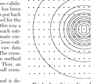
were estimated for rectangular blocks centered at each sample point. In 1995 fairways, the blocks mea-sured 4.6 by 14 m, and in 1996 the blocks were 4.6 by 7 m. Mean population densities were estimated for each block by 3 methodsÑmoving averages, inverse distances, and block kriging. For moving averages, estimates were made for all sampled blocks with smoothing radii of 0, 5.5, 7.6, 8.9, 10.7, 12.2, 14.2, 15.7, 18.8, 22.7, 31, and 47 m as indicated in Fig. 1. As discussed below, we used cross validation to deter-mine the optimum radii for each fairway. For inverse distances, estimates were made for all sampled blocks, using inverse distance exponents of P 5 0, 0.5, 0.75, 1, 1.25, 1.5, 1.75, 2, 2.5, 3, 3.5, 4, 4.5, and 5. An exponent of P 5 0 implies that all points receive the same weight, so estimates of all local means are equal to the overall mean. As p 3 `, the estimates of block means ap-proach the raw grub counts. As discussed below, we used cross validation to determine the optimum ex-ponent for the various fairways. For block kriging, omnidirectional and directional covariance models were used to obtain omnidirectional and directional block kriging estimates of local means, respectively.
Fig. 1. Smoothing radii used in calculation of moving
Effectiveness of Estimation of Local Means.
Cross-validation estimates were made for each fairway for inverse distances with each of the exponents, for mov-ing averages with each of the radii, and for both om-nidirectional and directional kriging.
Quanitification of Cross-Validation Errors.The mag-nitude of the cross-validation errors for a given set of estimates was measured 2 waysÑas the sum of squared errors (SSE), and as sums of absolute values of errors (SAE). The following standardizations of SSE and SAE were then made:
mean squared error: MSE 5(~zi*2 zi!
2
n , [2]
mean absolute error: MAE 5(?zi*n2 zi?, [3]
coefÞcient of determination: R25SST 2 SSE
SST , [4]
relative absolute error (analog of R2):
A 5SAT 2 SAESAT , [5] where zi*is the cross-validation estimate of sample i; ziis the number of grubs in sample i; n is the total
number of samples on the fairway; and SST and SAT are total sums of squared and absolute errors (i.e., the SSE and SAE for the null model, in which the overall mean is taken as the estimate for each local mean). Thus, MSE and MAE measure the average magnitude of errors, and R2and A are measures of the improvement
a given model makes over the null model, with values of 0 indicating no improvement, 1 indicating a perfect model, and negative numbers indicating a poorer Þt than than that of the null model.
Optimization.For each fairway, the moving average radius and inverse distance exponent that minimized the cross-validation MSE and MAE were selected as the optimum parameters. To make the Þnal MSE-op-timized and MAE-opMSE-op-timized estimates for a fairway, the moving average and inverse distance calculations were repeated using the optimum parameters with all the sample points on the fairway. Kriging estimates are based on models of the covariograms rather than on minimization of validation errors, but the cross-validation errors still were calculated for each fairway for comparison with the other methods.
Relative Effectiveness.To facilitate comparisons of the methodsÕ effectiveness among fairways, the R2and Avalues (equations. 4 and 5) for each method were standardized for each fairway by dividing by the R2
and A for directional kriging on that fairway. This is a measure of relative effectiveness based on a common scale for all fairways and methods. Thus, the relative effectiveness of directional kriging for both MSE and MAEfor each fairway is 1, and the other methods are compared against this standard. For example, a rela-tive MSE of 0.7 for a method implies that the method was 70% as effective as directional kriging at improving onthenullmodelÕsMSE,orR2
method/R2directionalkriging5
0.7. Because results are independent of which method is used as a standard, our choice of directional kriging was based solely on esthetic reasons.
Stability of the Methods. We deÞned stability of
moving averages and inverse distances in terms of the changes in estimates of local means for small changes in moving average smoothing radius or inverse dis-tance exponent.
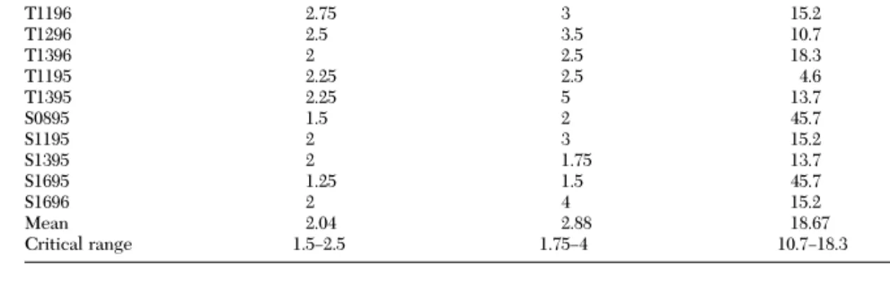
Critical Range of Parameters.For each fairway, we calculated the optimum exponent for inverse distance and optimum radius for moving averages by selecting the values that resulted in the smallest cross-validation MSE and MAE. We then removed the highest and lowest values and deÞned the critical range of param-eters to be the remaining interval. For example, the MSE-optimized inverse distance exponents for the twelve fairways were 1.25, 1.5, 1.75, 2, 2, 2, 2, 2.25, 2.25, 2.25, 2.5, and 2.75. After removing the highest and lowest of these exponents, the truncated range is 1.5Ð 2.5. This, then, was the critical range for MSE-opti-mized inverse distance. Similarly, we calculated the critical ranges for MAE-optimized inverse distance, MSE-optimized moving average, and MAE-optimized moving average. As deÞned, the critical range is an estimate of the range of optimum parameter values that were commonly observed in the Þeld. A method that can be standardized reliably should give consis-tent results for any choice of parameter value in the critical range.
Stability Index.The degree of smoothness of the grub density surface is summarized by a statistic that we refer to as the estimated population variance, or the variance of the collection of estimated local means for a given fairway and method. A high population vari-ance corresponds to a highly variable or rough surface, whereas a low population variance corresponds to a smooth surface. To quantify stability, we deÞned a stability indexfor a given fairway as the ratio of pop-ulation variances resulting from the highest and lowest parameter values in the critical range. For example, the critical range for MSE-optimized inverse distance exponents is 1.5Ð2.5. The estimated population vari-ances on T1896 for exponents 1.5 and 2.5 are 0.17 and 0.58, respectively, so the stability index for MSE-opti-mized inverse distance on T1896 is 0.58/0.17 5 3.4. By contrast, the critical range for MSE-optimized moving average radii is 10.7Ð18.8 m. The estimated population variances on T1896 for radii 18.8 and 10.7 are 0.31 and 0.21, respectively, giving a stability index of 1.5. By this measure, the inverse distance method has a higher stability index value and is more unstable than moving averages on fairway T1896. We calculated stability indices for both inverse distances and moving averages optimized for MSE and MAE on all 12 fairways ana-lyzed.
Critical Ratio and Quantification of the Practical Im-plications of the Stability Index.Because of space lim-itations, the nature and degree of the uncertainties captured by the stability index were analyzed in detail for only 1 fairway (T1896). Differences in grub density surfaces for parameters within the critical range for MSE-optimized inverse distance exponents and
mov-ing average radii were plotted in wireframe graphs of estimated local mean populations. The wireframe graphs provide a visual summary of the practical im-portance of the stability index. Differences between the surfaces then were quantiÞed via differences in the heights and extents of the peaks. The peaks were characterized by the upper percentiles (50th, 75th, 90th, 95th, 98th, and maximum) of the estimated local means on the fairway. These percentiles were then plotted as functions of the inverse distance exponent and moving average radius. Of particular interest were the differences in the estimates of each percentile for parameters within the critical range. To summarize such differences, we deÞned the critical ratio for a given method and percentile on a fairway as the ratio of the highest to the lowest estimate of the percentile for parameter values in the critical range. For example, the estimates for the 98th percentile of block means on T1896 for inverse distance exponents of 1.5 and 2.5 (spanning the critical parameter range) are 1.58 and 2.73, respectively. Therefore, the 98th percentile crit-ical ratio for inverse distances on T1896 is 2.73/1.58 5 1.73, implying that within the critical range, estimates of the 98th percentile vary by a factor of 1.73. For each fairway the critical ratio was calculated for inverse distances and moving averages, each optimized for MSEand MAE. Then for each method, the geometric mean critical ratio across fairways was calculated and plotted against percentile. We used the geometric mean whenever calculating an average of ratios or factors. The geometric mean considers1⁄2and 2 to be
equidistant from 1, an apt view when dealing with factors and ratios. This allows for easy comparison of the robustness of the methodsÕ estimates of the heights of the peaks and how those estimates depend on rel-ative grub population density.
Fairway Selection. Detailed spatial statistical
anal-yses were performed on 12 of 18 fairways sampled. Not included were 2 fairways that lacked signiÞcant spatial covarianceÑS1396 had a mean grub density of 0.15 per sample, and the count distribution did not differ from Poisson (P 5 0.18, chi-square test); S0896 had a mean grub density of 0.27 per sample, and neither the variogram nor covariogram revealed any spatial co-variance structure. Not coincidentally, these 2 fair-ways had the lowest and 4th lowest population den-sities of the 18 that were sampled; not enough grubs were found to discern spatial relationships. Also not included in the analyses were 4 fairways for which the spatial covariance was not strong enough for any of the methods to provide reliable estimates. As a rough measure of reliability, we used the P value of the linear regression of cross-validation estimates against the raw grubs counts. Fairways T1895, T1095, T1295, and S1196 had P values substantially higher than those of the other fairways (Fig. 2), making meaningful com-parisons between the methods impossible for these 4 fairways. Therefore, the analysis does not include these fairways.
Results and Discussion
Effectiveness. The relative effectiveness of the
methods (inverse distance, moving average, omnidi-rectional kriging, diomnidi-rectional kriging) was compared on the basis of the MSE and MAE of the cross-valida-tion errors. For each fairway, the inverse distance exponent and moving average radius that minimized the MSE and MAE were calculated and are listed in Table 3. Optimum parameter values varied not only from fairway to fairway but also depended on whether they were optimized with respect to MSE or MAE. For inverse distances and moving averages, the analysis of effectiveness was based on these optimized parame-ters.
Effectiveness of Moving Averages and Inverse Dis-tances Relative to Directional Kriging. On average, MSE-optimized inverse distances and moving aver-ages were respectively only 82 and 67% as effective as directional kriging at improving on the null MSE. In Fig. 3 points above the dotted line represent a relative effectiveness .1, indicating that the given method is more effective than directional kriging on the fairway represented by the point. Conversely, points below the dotted line indicate that the method is not as effective as directional kriging on the fairway. When compared on the basis of MAE rather than MSE, in-verse distances and moving averages were still not as effective as directional kriging, although the differ-ences were less pronounced (geometric means of rel-ative effectiveness were 85 and 90% for inverse dis-tances and moving averages, respectively).
For all but 1 fairway (S1696), directional kriging was the most effective as measured by MSE. For S1696, inverse distance with an exponent of 2 had a relative effectiveness of 1.35 (optimized for MSE). However, the methodÕs R2 was still only 0.047 compared with Fig. 2. Fairway-by-fairway P values for linear regression
of cross-validation residuals on sample grub counts. For fair-ways T1895, T1095, T1295, and S1196, the correlations are substantially weaker than they are for the other fairways, indicating that none of the estimation methods is reliable on these data sets.
directional krigingÕs 0.035 (Table 4), implying that both methods were only slightly better than the null model in which all local means are assumed to be equal to the overall mean. The relative effectiveness of mov-ing average optimized for MAE is 1.9 for the same fairway, indicating that the method outperformed di-rectional kriging on this fairway. For all other fairways, directional kriging was the most effective with respect to MSE (Fig. 3; Table 4). However, inverse distance and moving average often were much less effective than directional kriging. On 5 of the 12 fairways, MSE-optimized inverse distances were ,75% as effective as directional kriging, and on 6 fairways MSE-optimized moving averages were ,70% as effective as directional kriging. On 1 fairway (T1195), MSE-optimized moving averages were outperformed by the null model.
The relative effectiveness of inverse distances and moving averages improved when MAE was the yard-stick. The improved performance relative to kriging is
not surprising in that inverse distances and moving averages can be optimized to give low MAE, whereas kriging inherently minimizes MSE rather than MAE. On S1696, moving averages had substantially higher relative effectiveness than all other methods (Fig. 3). This may be because the low mean population density on the fairway (0.23 grubs per sample compared with an average of 1.01 for the other fairways with signif-icant spatial covariance) (Table 1). Only 37 of 225 samples contained grubs. Because the sampling pro-vided so little information about the grub dispersion patterns, the results are highly sensitive to random variation, so the unusually strong performance of mov-ing averages is probably overstated by the relative effectiveness statistic. On 4 other fairways (T1096, T1196, T1296, and T1396) moving averages yielded the lowest MAE of all the methods, although the perfor-mances were only slightly better than directional krig-ing (Fig. 3; Table 4). On all other fairways, directional kriging was still the most effective as measured by MAE. On several of these fairways, the differences were large.
In summary, we found that although on some fair-ways the effectiveness of directional kriging was not signiÞcantly better than that of inverse distances or moving averages, directional kriging greatly outper-formed the other methods on a third to half of the fairways.
Effectiveness of Omnidirectional Kriging Relative to Directional Kriging.Incorporating the effect of tion into covariogram models when performing direc-tional kriging greatly complicates the modeling effort. In most cases, the added complexity did not result in signiÞcantly better estimates of local means, because on most fairways omnidirectional kriging was as ef-fective or nearly as efef-fective as directional kriging. On 9 of the 12 fairways, omnidirectional kriging was .90% as effective as directional kriging at improving on the null MSE (Fig 3). On fairways S1695, S0895, and T1396, however, omnidirectional kriging had MSE-based rel-ative effectiveness of 0.48, 0.72, and 0.82, respectively, indicating that directional kriging was substantially more effective on these fairways. As measured by MAE,the performance gap between omnidirectional
Fig. 3. Relative effectiveness of moving average, inverse
distance, and omnidirectional kriging using directional krig-ing as a standard for comparison. Each dot represents the relative effectiveness of the method indicated on the x-axis for a single fairway. Inverse distance exponents and moving average radii are optimized for MSE and MAE of cross-vali-dation errors, as indicated. Open squares represent geomet-ric means. Points above and below the dotted line represent superiority over and inferiority to directional kriging.
Table 3. Inverse distance and moving average parameters that minimize MAE and MSE
Fairway Inverse distances, exponent: Moving averages, Radius m
MSE-optimized MAE-optimized MSE-optimized MAE-optimized
T1896 1.75 2.75 15.2 8.8 T1096 2.25 3 10.7 10.7 T1196 2.75 3 15.2 7.6 T1296 2.5 3.5 10.7 10.7 T1396 2 2.5 18.3 8.8 T1195 2.25 2.5 4.6 4.6 T1395 2.25 5 13.7 7.6 S0895 1.5 2 45.7 10.7 S1195 2 3 15.2 7.6 S1395 2 1.75 13.7 13.7 S1695 1.25 1.5 45.7 10.7 S1696 2 4 15.2 7.6 Mean 2.04 2.88 18.67 9.09 Critical range 1.5Ð2.5 1.75Ð4 10.7Ð18.3 7.6Ð10.7
and directional kriging was smaller than when mea-sured by MSE (Fig. 3). On 10 of the 12 fairways, the relative effectiveness of omnidirectional kriging ex-ceeded 90% as measured by improvement in MAE over the null model.
Stability. The main advantage that inverse distances
and moving averages have over kriging is ease of cal-culation. We found that, when optimized, inverse dis-tances and moving averages were sometimes compa-rable to directional kriging with respect to effectiveness. However, optimization is calculation-intensive and thus partially negates the advantage of simplicity. Therefore, as others have noted (e.g., Weisz et al. 1995a, b), it would be highly beneÞcial to be able to use a single, standard parameter that would be applicable to all Þelds. However, as discussed be-low, we found that such standardization would con-tribute substantially to the uncertainty of the esti-mates made by inverse distances and moving averages. Stability Index for Moving Averages and Inverse Dis-tances.We quantiÞed the degree of uncertainty asso-ciated with choosing a standard inverse distance ex-ponent or moving average radius for use on all fairways by use of the stability index (Table 3). An unstable method is not amenable to standardization because the standard parameter is likely to differ enough from the optimum to have a signiÞcant impact on the re-sulting estimates of local means.
Moving averages were more stable than inverse distances on the fairways we sampled (Fig. 4). The stability index for MSE-optimized inverse distances exceeded 3.0 on 11 of 12 fairways, whereas the index for MSE-optimized moving averages was ,3.0 for 11 of the 12 fairways. The differences in stability between inverse distances and moving averages optimized for MAEwere even greater. The stability index for MAE-optimized inverse distances exceeded 3.0 for all 12 fairways, whereas the stability index for MAE-opti-mized moving averages was ,1.8 for all 12 fairways. Thus, the method of inverse distances was less well suited for standardization than was moving averages. Not only was the method of inverse distances less well suited for standardization than was moving
av-erages, we also found the method to be unsuitable in an absolute sense. The argument relies on a more detailed discussion of the practical signiÞcance of the stability index. Because of space limitations, we limit the detailed discussion to 1 fairway. Fairway T1896 with inverse distances with MSE optimization was selected because it has a stability index of 3.44, which marks a cutoff that separates inverse distances from moving averages with respect to stability (Fig. 4). T1896 is among the most stable fairways for inverse distances, yet its stability index value of 3.44 for MSE is higher than the index for moving averages on every fairway (Fig. 4; Table 5).
Stability Index and Uncertainty of Topography of the Grub Density Map. A stability index of 3.44 corre-sponds to a large degree of uncertainty about the roughness of the estimated grub density surface, as shown in Fig. 5a and b However, an index of 3.44 is close to the minimum for inverse distances among all fairways. The density surfaces for most of the fairways Table 4. Effectiveness of methods of estimating local mean populations
Cross-validation R2 Cross-validation A IDa MAb OKc DKd IDa MAb OKc DKd T1896 0.125 0.144 0.142 0.163 0.142 0.158 0.156 0.161 T1096 0.157 0.175 0.177 0.177 0.133 0.168 0.152 0.152 T1196 0.219 0.199 0.220 0.240 0.168 0.195 0.174 0.191 T1296 0.213 0.207 0.213 0.213 0.194 0.210 0.194 0.194 T1396 0.124 0.137 0.145 0.177 0.090 0.126 0.114 0.122 T1195 0.103 20.020 0.164 0.164 0.055 0.026 0.090 0.090 T1395 0.169 0.161 0.210 0.210 0.158 0.158 0.148 0.148 S0895 0.102 0.086 0.098 0.136 0.046 0.042 0.055 0.069 S1195 0.129 0.101 0.148 0.154 0.107 0.100 0.106 0.113 S1395 0.200 0.138 0.226 0.226 0.122 0.103 0.130 0.130 S1695 0.069 0.065 0.049 0.104 0.048 0.063 0.049 0.067 S1696 0.047 0.023 0.035 0.035 0.090 0.125 0.066 0.066
aInverse distance weighting. bMoving averages. cOmnidirectional kriging. dDirectional kriging.
Fig. 4. Stability index for moving averages and inverse
distances. Each dot represents the stability index for a single fairway and a given method (x-axis). The value of the index increases with uncertainty about the smoothness of the grub population density surface.
vary even more markedly for parameter values in the critical ranges (MSE and MAE) for inverse distances. By contrast, Fig. 5c and d illustrate the uncertainty associated with a stability index of 1.53, the value for MSE-optimized moving averages on the fairway. Thus, the moving average surfaces are relatively consistent for all radii in the critical range. The stability index is a general quantiÞcation of the differences visible in
Fig. 5, and as such, the index measures the relative stability of the methods. However, the practical implications of differences in stability are not cap-tured directly by the index. Instead, we examined the stability of the distribution of local means within the critical region for a quantitative assessment of the practical implications of a stability index value of 3.44.
Table 5. Estimated population variance and stability index (ratio)
Fairway
Inverse distance Moving avg
MSE MAE MSE MAE
p 5 1.5 p 5 2.5 Ratio p 5 1.75 p 5 4 Ratio r 5 10.7 r 5 18.8 Ratio r 5 7.6 r 5 01.7 Ratio T1896 0.168 0.578 3.441 0.249 1.054 4.228 0.314 0.205 1.529 0.446 0.314 1.421 T1096 0.146 0.657 4.500 0.241 1.248 5.170 0.381 0.229 1.665 0.543 0.381 1.427 T1196 0.420 1.332 3.170 0.599 2.368 3.955 0.790 0.549 1.439 1.116 0.790 1.412 T1296 0.076 0.393 5.183 0.132 0.774 5.873 0.241 0.135 1.789 0.348 0.241 1.443 T1396 0.140 0.570 4.072 0.218 1.115 5.121 0.317 0.185 1.716 0.474 0.317 1.494 T1195 0.270 1.170 4.324 0.454 2.133 4.702 1.028 0.307 3.348 1.738 1.028 1.691 T1395 0.177 0.614 3.476 0.273 1.021 3.737 0.662 0.234 2.829 0.873 0.662 1.318 S0895 0.381 1.039 2.728 0.539 1.646 3.056 1.081 0.424 2.550 1.393 1.081 1.289 S1195 0.131 0.618 4.720 0.226 1.141 5.042 0.636 0.272 2.336 0.933 0.636 1.467 S1395 0.408 1.249 3.066 0.600 2.020 3.368 1.369 0.579 2.365 1.808 1.369 1.321 S1695 0.171 0.530 3.104 0.249 0.895 3.588 0.560 0.199 2.812 0.758 0.560 1.355 S1696 0.027 0.153 5.618 0.048 0.320 6.684 0.058 0.030 1.919 0.102 0.058 1.767 Mean 0.210 0.742 3.950 0.319 1.311 4.544 0.620 0.279 2.192 0.878 0.620 1.451 Geometric mean Ñ Ñ 3.854 Ñ Ñ 4.428 Ñ Ñ 2.117 Ñ Ñ 1.444
Fig. 5. Estimated grub population density on fairway T1896 using inverse distances and moving averages with parameter
values in the critical range. (A) Inverse distance with exponent of 2.5. (B) Inverse distance with exponent of 1.5. (C) Moving average with radius of 10.7 m. (D) Moving average with radius of 18.3 m.
Stability Index and Uncertainty of Patch Density.The overall mean grub density for the surfaces in Fig. 5a andb is essentially the sameÑ0.676 for exponent 1.5 and 0.667 for exponent 2.5. The differences between the surfaces lie in the heights of the peaks and the depths of the troughs. The sizes of the peaks can be compared via the upper tails of the distributions of local means. In Fig. 6, a given percentile of estimated local grub density is plotted against inverse distance exponent p. The lowest line is the estimated minimum grub density. Lines for the median, 75th, 90th, 95th, and 98th percentiles are above that, with the line for the maximum on top. For p 5 0, all local means are equal to the overall sample mean, so the lines start at the local mean and spread out as p increases. Steepness in the curve is indicative of rapid change in grub density surface corresponding to relatively small changes in exponent. For example, with an exponent of 1.5, the estimated maximum population density is 1.99, but for an exponent of 2.5, the expected maxi-mum rises to 3.94, nearly twice as high. Thus, within the critical range for MSE, estimates of the maximum grub density on the fairway vary by nearly a factor of 2, making inverse distances unreliable for estimating the maximum population density on this fairway.
Stability Index and Uncertainty About Patch Extent. A turfgrass manager interested in treating only those sections of the fairway that harbor grub patches with density exceeding a threshold would need to identify the boundaries of those patches. A commonly used treatment threshold for Japanese beetle grubs in turf-grass is 100 grubs per square meter, or '1 per sample. According to inverse distance with an exponent of 1.5, 21% of the fairway (T1896) has a density exceeding 1 and would be treatable. With an exponent of 2.5, the
treatable fraction of the fairway rises only to 23%. This indicates that for T1896, choice of exponent within the critical range has very little effect on the estimation of the treatable portion of the fairway given a treatment threshold of 1 grub per sample, making inverse dis-tance a seemingly reliable tool. For a treatment thresh-old of 1.5, however, the situation changes dramatically. An exponent of 1.5 results in an estimate of 2.8% of the fairway requiring treatment. An exponent of 2.5 in-creases the estimated treatable portion of the fairway to 17%, a 6-fold increase, making inverse distance an unreliable tool for identifying patch boundaries. Fig. 6 suggests that inverse distance gives a consistent es-timate of the 75th percentile of grub density on T1896. However, it gives inconsistent estimates of the upper quantiles of population density. Thus, a stability index of 3.44 or higher is a strong indication that the method may be unreliable for many types of ecological prob-lems. Because the stability index was commonly in excess of 3.44 for inverse distances (both for MSE and MAE), the method was not suitable for standardization by using a single exponent for all fairways.
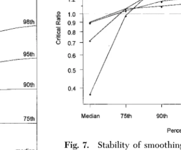
Suitability of Standardization of Inverse Distance and Moving Averages.As alluded to in the previous para-graph, suitability for standardization is dependent upon the question of interest. Fig. 7 shows how the upper tail of the distribution of estimated local means (i.e., the heights of the peaks) varies for parameters in the critical range. We deÞned the critical ratio for a method as the ratio of the estimates of a given grub density percentile for parameters on the boundaries of the critical range. The critical ratio was calculated for each fairway for inverse distances and moving aver-ages for a number of percentiles. The average critical ratio in Fig. 7 is the geometric mean of the ratios for all the fairways, and it is a measure of how stable a
Fig. 6. Percentiles of estimated local mean grub densities
on fairway T1896 as functions of inverse distance exponent. Vertical lines represent the boundaries of the critical param-eter range.
Fig. 7. Stability of smoothing methods with respect to
distribution of local means. A critical ratio near 1.0 indicates that the method gives consistent estimates of the given per-centile for all parameters in the critical range. ID, method of inverse distances; MA, moving averages; mae and mse denote which critical range (MSE or MAE) was used to calculate the critical ratios. Critical ratios are the mean critical ratios across all fairways.
given method is for estimating a given quantile on average. Thus, Fig. 7 shows that the least stable method on average is inverse distance optimized for MAE. Within the critical parameter range for this method, estimates of the median vary by a factor of 2.7, which is far higher than for any other method. All the methods reliably estimate the 75th percentile on av-erage, but the critical ratio for MAE-optimized inverse distance estimates is 1.5 or more for the 90th percen-tile and above and exceeds all other methods at every percentile higher than the 75th. The critical ratios for moving averages (optimized for either MSE or MAE) are between 0.8 and 1.25 for all quantiles between the median and 95th percentile. The most stable method is moving averages optimized for MAEÑall critical ratios are between 0.8 and 1.25.
In summary, without optimization, the inverse dis-tance method was too unstable to reliably estimate the median population density, upper percentiles (or heights of the peaks on the grub density maps), or maximum local means. Even when optimized for MSE or MAE, cross-validation indicates that the inverse distance method is less effective than directional krig-ing at estimatkrig-ing local means.
The method of moving averages was more stable than inverse distances; it may even be stable enough for a standard radius to be used for some applications, especially when the standard is based on the minimi-zation of MAE. Moving averages optimized for MSE was considerably less effective than either directional or omnidirectional kriging; but when optimized for MAE,it was often comparable in effectiveness to om-nidirectional kriging.
Directional kriging consistently gave better esti-mates of local means than either moving averages or inverse distances when measured by MSE. When mea-sured by MAE, moving averages gave slightly better estimates than directional kriging on some fairways, but on 25% of the fairways, it was substantially out-performed by directional kriging.
Natural variation in the spatial patterns of grub abundance from fairway to fairway and year to year was great enough that selection of a standard exponent for inverse distances or a standard smoothing radius for moving averages often resulted in poor estimates of local means, especially in sections of fairways where grub density was relatively high. When the variation in grub patterns was implicitly accounted for by op-timization of exponent or smoothing radius on a fair-way-by-fairway basis, the stability and effectiveness of moving averages and inverse distances improved, but only with an increase in complexity. Moreover, even with optimization, inverse distances and moving av-erages were still far less effective than kriging for several fairways.
In conclusion, we demonstated that in some situa-tions standardized inverse distances or moving aver-ages may perform just as well or nearly as well as directional kriging, whereas for other situations, the
methods may be vastly outperformed by kriging, even after they are optimized. Their performance on a par-ticular data set depends on whether the spatial co-variance of the data by chance happens to be com-patible with the inverse distance or moving average model. Therefore, inverse distances and moving av-erages tend to be unreliable, even though they occa-sionally may be just as effective as directional kriging. Because kriging is linked to the ecology of the organ-ism via an explicit model of the spatial covariance, it naturally adjusts itself to the spatial patterns in the data and therefore performs more consistently and reliably than inverse distances or moving averages. Because of its higher degree of reliability, kriging is to be recommended over inverse distances or moving averages for estimation of local means.
Acknowledgments
We thank Nancy Consolie for stellar technical assistance in the Þeld, Lisa Madsen for statistical advice and assistance, and Dave Benarski and Norm Sharman for their generous cooperation in allowing us to sample their golf courses. This study was supported by funds from USDAÐNRI, Northeast Regional Integrated Pest Management (IPM), NY State IPM, USGA, Musser International Turfgrass Foundation, and the Cornell University Departments of Entomology (Geneva and Ithaca, NY).
References Cited
Cressie, N.A.C. 1993. Statistics for spatial data. Wiley, New York.
Deutsch, C. V., and A. G. Journel. 1992. GSLIB: geostatis-tical software library and userÕs guide. Oxford University Press, New York.
Isaaks, E. H., and R. M. Srivastava. 1989. Applied geostatis-tics. Oxford University Press, New York.
Kaluzny, S. P., S. C. Vega, T. P. Cardoso, and A. A. Shelly. 1996. S1SpatialStats userÕs manual. MathSoft, Seattle, WA. Midgarden, D., S. J. Fleischer, R. Weisz, and Z. Smilowitz.
1997. Site-speciÞc integrated pest management impact on development of esenvalerate resistence in Colorado potato beetle (Coleoptera: Chrysolmelidae) and on den-sities of natural enemies. J. Econ. Entomol. 90: 855Ð867. Nyrop, J. P., M. G. Villani, and J. A. Grant. 1995. Control de-cision rule for European chafer (Coleoptera: Scarabaeidae) larvae infesting turfgrass. Environ. Entomol. 24: 521Ð528. Weisz, R., S. Fleischer, and Z. Smilowitz. 1995a.
Site-spe-ciÞc integrated psest management for high value crops: sample units for map generation using the Colorado po-tato beetle (Coleoptera: Chrysomelidae) as a model sys-tem. J. Econ. Entomol. 88: 1069Ð1080.
1995b. Map generation in high-value horticultural inte-grated pest management: appropriate interpolation methods for site-speciÞc pest management of Colorado potato beetle (Coleoptera: Chrysolmelidae). J. Econ. En-tomol. 88(6): 1650Ð1657.
Received for publication 17 April 1998; accepted 23 October 1998.
Appendix 1: Determination of Inverse Distance Weights for Center Points of Blocks.
Because samples are taken at the center of each block, an inverse distance weighting would give each sample inÞnite weight in the determination its block mean. The estimates of the block means would simply be the raw sample values. Because the problem is to estimate the mean in a small area, a possible alternative would be to make conventional, interpolated inverse distance estimates for a number of points in each block. The block mean estimate would be then be the average of the interpolated point estimates. This proposed solution has 2 drawbacks as follows: (1) it substantially increases the difÞculty of the computa-tions in terms of computer memory and CPU time; (2) limmin?x2xo?30~mˆo! 5 v0, or as more and more points
are averaged, the estimated mean approaches the raw sample count. The 1st drawback is overcome by noting that averaging a Þnite number of interpolated points in a block is equivalent to assigning a proper weight to the central point. The ideal weight varies with the number of interpolated points, the size of the block, and the inverse distance exponent. Problem (2) is overcome by taking a moderate number of interpo-lated points for each block size. For powers between 0.5 and 5 and for an equally spaced grid of 16 inter-polated points within a block, the ideal weight is
be-tween the arithmetic mean and the harmonic mean of the weights that assigned to the 16 points by their inverse distance to the center of the block. The ideal weight never varies far from the geometric mean, so that is the weight we use throughout the study. Thus, the preliminary weights given to individual central samples in the estimation of the mean density in their respective blocks are given in Table 2 (these weights are the wjÕs in equation 1).
Table 2. Weights assigned to samples at centers of blocks for inverse distance method
Power Weight a 4.6 by 7 m. grid 4.6 by 14 m. grid 0.5 0.3901 0.3074689 0.75 0.2437 0.170491 1 0.1522 0.094537 1.25 0.09507 0.052421 1.5 0.05938 0.029067 1.75 0.03709 0.016118 2 0.02317 0.0089373 2.25 0.01447 0.004956 2.5 0.009038 0.002748 2.75 0.005645 0.001523 3 0.003526 0.00084490 3.5 0.001376 0.0002598 4 0.0005367 0.00007987 4.5 0.0002094 0.00002456 5 0.00008169 0.000007551
aWeights are the w