HAL Id: hal-00617477
https://hal.univ-brest.fr/hal-00617477
Submitted on 29 Aug 2011HAL is a multi-disciplinary open access archive for the deposit and dissemination of sci-entific research documents, whether they are pub-lished or not. The documents may come from teaching and research institutions in France or abroad, or from public or private research centers.
L’archive ouverte pluridisciplinaire HAL, est destinée au dépôt et à la diffusion de documents scientifiques de niveau recherche, publiés ou non, émanant des établissements d’enseignement et de recherche français ou étrangers, des laboratoires publics ou privés.
Application of free sorting tasks to sound quality
experiments
Etienne Parizet, Vincent Koehl
To cite this version:
Etienne Parizet, Vincent Koehl. Application of free sorting tasks to sound quality experiments. Ap-plied Acoustics, Elsevier, 2012, 73 (1), pp.61-65. �10.1016/j.apacoust.2011.07.007�. �hal-00617477�
TITLE :
Application of free sorting tasks to sound quality experiments
AUTHORS :
Etienne PARIZET
Laboratoire Vibrations Acoustique, Insa-Lyon, 25 bis avenue Jean Capelle, 69621
Villeurbanne Cédex, France
[email protected] Vincent KOEHL
Université de Brest, LISyC EA 3883, Centre Européen de Réalité Virtuelle, 25 rue Claude
ABSTRACT
In many studies devoted to the sound quality of industrial products, a perceptual space is
determined through dissimilarity judgements on pairs of stimuli. A drawback of this
procedure is that it can be very time consuming if the number of stimuli is large. An
alternative procedure consists in a free sorting of sounds: averaging individual results
provides a set of data which are considered as indicators of dissimilarities and analyzed
using a multi-dimensional scaling method. The validity of this alternative can be discussed,
as the psychological processes involved in the two procedures are different.
This study compared these two approaches in a particular case (door closure sounds). In
this specific case, it was observed that dissimilarities obtained from the two procedures can
be different, the more so as sounds are dissimilar and these differences can lead to slightly
different perceptual spaces. Nevertheless, a free sorting experiment is a reliable way of
reducing the number of stimuli in a large set of sounds. It allows selecting some
representative sounds and narrowing the set of sounds while keeping in the subset most of
the timbre features. This provides a useful preliminary step to a paired-comparison
experiment.
1. INTRODUCTION
In sound quality applications, the identification of important timbre features is a key factor.
This knowledge allows the selection of sound metrics which can be used as input of a
preference model. It also gives useful indications about the way the object should be
modified in order to improve its sound quality. Numerous methods can be used to identify
these attributes; a very common one consists in asking subjects to evaluate the dissimilarity
between two sounds presented by pairs. After collecting the individual data,
multi-dimensional techniques lead to a perceptual space, in which stimuli can be placed so that
their relative distances are close to their perceived dissimilarities. The axes of this space can
then be related to timbre features, as implicitly used by listeners when achieving the task.
These timbre features are inferred by the experimenter (e.g. by listening to sounds with very
different coordinates along this axis, or by computing correlations between these coordinates
and candidate sound metrics, as loudness, sharpness and so on). Such a procedure has been
widely used in many applications: sounds from musical instruments (Kendal and Carterette,
1991), synthesized ones (McAdams et al. 1995), car sounds (Lemaître et al., 2004, Parizet et
al., 2007), aircraft noise (Barbot et al., 2008) as examples. A major drawback of this
procedure lies in the number of pairs to be presented to the listener, which is a square
function of the number of sounds. This can make the experiment very long and tedious for
the listener.
Another procedure consists in free sorting experiments. Subjects are asked to group stimuli
together, on a similarity basis; they can make as many groups as they want to. This task is
related to categorization process. But the relation between categorization and similarity
evaluation is strong (Thibaut, 1997), though some exceptions have been pointed out (see
Rips, 1993, for an example). Individual results are co-occurrence matrices, made of 0 and 1
co-occurrence matrices provides a matrix which is considered as a dissimilarity one, and, as
such, can be analyzed thanks to a multi-dimensional technique. Various examples can be
given, in the field of visual perception (see Börner, 2000 or Faye et al., 2004), haptic
perception (Picard et al., 2003 or Tiest and Kappers, 2006), food evaluation (Falahee and
MacRae, 1997), or perception of everyday life situations (Edwards and Templeton, 2005). In
the field of sound perception, this kind of analysis was realized in the case of environmental
sounds (Guastavino, 2003, Dubois et al., 2004), everyday sounds (Guyot et al., 1997, Houix
et al., 2008), cars dashboard tapping sounds (Montignies and Parizet, 2008) or loudspeakers
quality (Lavandier et al., 2005). In spite of the advantage of such a procedure, a question
should be kept in mind: as the task of listeners does not consist in evaluating dissimilarities
between sounds, can averaged data be considered as dissimilarities? Will the perceptual
space obtained from these data be close to the one obtained from real dissimilarities? For
sound stimuli, only one published study compared results obtained from these two methods
(Bigand et al., 2005). This study used musical excerpts as stimuli and showed a good
agreement between results. The goal of this paper is to present another example, using
another kind of sounds (car door closure sounds), and to discuss how free sorting
experiments can be used in typical sound quality applications. Three experiments have been
conducted:
- in the first one, a set of 35 sounds was sorted by listeners; this allowed to split this set in 6
groups of similar sounds;
- in the second experiment, 12 sounds extracted from this set (2 sounds for each group) were
sorted, using the same procedure. It appeared that stimuli could still be clustered in 6 groups,
indicating that the organization of sounds, as determined from the first experiment, was
- finally, in a third experiment, subjects were asked to evaluate dissimilarities between the
same 12 sounds presented by pairs. The perceptual spaces obtained from the results of this
experiment and the previous one proved to be slightly different.
The comparison of the results of these three experiments will provide some guidelines about
the way a free sorting experiment can be used in such applications.
2. EXPERIMENT 1 : FREE SORTING OF 35 SOUND SAMPLES
2.1. Stimuli
Car door closure sounds were used in that experiment; they were part of a study presented in
another paper (Parizet et al., 2007). At the beginning of this study, 16 cars were used. Each
car was entered in a semi-anechoic room and the driver's door closure sound was recorded
with a dummy head (Bruel et Kjaer type 4133) placed outside the car, in the typical position
of the driver leaving the car. Sounds were sampled at a 16-bits resolution with a 44.1 kHz
sampling frequency. Some modifications of the door seals were realized on two cars,
increasing the number of stimuli to 27. Finally, for 8 situations, a second recording of the
closing was introduced in the set of sounds in order to check the repeatability of
measurements. Thus the overall number of stimuli was 35. Their duration was of
approximately one second.
2.2. Free sorting experiment
Sounds were presented to listeners through headphones in a quiet room. Subjects were
similar sounds, forming as many groups they wanted to. They could listen to sounds as many
time as they felt necessary.
31 subjects participated to the experiment (students or staff member of the laboratory).
2.3. Results
For each listener, a 35 x 35 co-occurrence matrix was determined. Each cell of this matrix
was 0 if the two corresponding sounds had been placed in the same group by the listener, 1
otherwise. First of all, the importance of inter-individual variability was evaluated. Using
Rand Index as an indicator of agreement between two individual clusterings (Hubert and
Arabie, 1985), it was not possible to separate the panel into sub-groups of listeners.
Therefore, all individual co-occurrence matrices were averaged, which lead to a dissimilarity
matrix. The values of this matrix ranged between 0 and 1. It should be noted that data thus
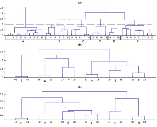
obtained are real distances, as they fulfil the triangle inequality ( , )d x z ≤d x y( , )+d y z( , ). A hierarchical clustering using Ward's method (Saporta, 2006, p. 258) was computed and
lead to the dendrogram presented in figure 1.a. In this diagram, the vertical axis represents
distance between stimuli: the higher the node between two stimuli, the larger the distance
between them. It was decided to split up the set of sounds in six groups, represented on that
figure. It can be noted that, when two recordings of the same door were included in the set of
sounds, they belonged to the same group (these repetitions are labelled as (2-3), (7-8),
(9-10), (11-12), (20-21), (25-26), (29-30) and (31-32)).
For the following of the study, two sounds were selected in each group. The selection rule
was the following one : for each sound, the average dissimilarity between this sound and all
the other ones belonging to the same group was computed. The two sounds leading to the
are labelled as 18 and 30 (for group A), 3 and 6 (group B), 8 and 27 (group C), 13 and 16
(group D), 9 and 28 (group E), 26 and 32 (group F).
3 EXPERIMENT 2 : FREE SORTING OF 12 SOUND SAMPLES
3.1. Experimental procedure
The 12 sound samples selected from the previous experiment were used. 30 subjects
participated to a second free sorting experiment. They had to group these 12 sounds in
clusters, using the same procedure as in the first experiment (and the same playback
conditions). They were members of the laboratory (staff and students). Only 8 of them had
participated in the first experiment (which had taken place more than one year before that
one).
3.2. Results
Individual results were collected and analyzed as in the previous experiment. Subgroups of
listeners could not be built, so that the mean dissimilarity matrix was computed from all
subjects. The dendrogram obtained from the hierarchical clustering analysis of this matrix is
shown on figure 1.b. It can be seen that the set of sounds can be organized in the same 6
groups. Therefore, it seems that the structure underlying the set of sounds used in the first
experiment was preserved by the selection of representative sounds.
4 : EXPERIMENT 3 : DISSIMILARITY RATINGS, 12 SOUND SAMPLES
4.1. Experimental procedure
The same set of 12 sounds was used in a dissimilarity experiment. After listening to each
pair of sounds, the listener had to evaluate the dissimilarity between the two stimuli, and to
equal" to "sounds are extremely different". 40 people took part in this experiment. As
required by the car supplier funding this part of the study, listeners did not belong to the
laboratory and the jury was balanced in two ways. First of all, it was made of 19 women and
21 men. Then, in each gender group, half of the subjects were between 30 and 45 and the
other onesbetween 46 and 60.
This experiment provided a set of individual dissimilarities, recorded as numbers varying
between 0 and 1; there were 40 x 66 such values, as 66 pairs (representing the upper half of
the 12x12 matrix) were presented to each listener.
4.2. Results
As in the previous experiment, no clustering of listeners could be made. Differences between
groups of subjects (age and gender) were not significant, and a hierarchical clustering
analysis did not allow building groups of subjects from individual results. Therefore,
individual values were averaged to derive a mean dissimilarity matrix. A hierarchical
clustering analysis was conducted for that matrix and the result is presented in figure 1.c.
Once again, the 6 group structure can clearly be identified: this seems to be an actual
organization scheme of the sound samples and the selection of the representative sounds in
experiment 1 allowed to preserve this scheme. Nevertheless, some discrepancies between
dendrograms appear on figure 1. For instance, stimuli from the D group (labelled as 13 and
16) are closer to the A, E and F groups than to the C and B groups, while the reverse was
true in the previous experiment. Both experiments lead to the same 6-groups clustering, but
the overall structures of these groups are slightly different from one experiment to the other
one.
In the following, the comparison between experiments 2 and 3 (based on the same set of
5. COMPARISON OF EXPERIMENTS 2 AND 3
5.1. Comparison of dissimilarities
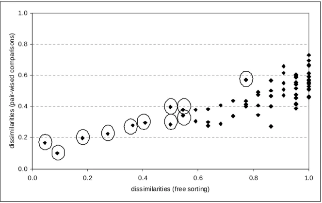
In each case, the averaged dissimilarities between sounds were computed. They are shown in
figure 2. Each point represents one of the 66 pairs of sounds. The X-axis coordinate of the
point is the distance between the two sounds as obtained from the free-sorting experiment
and its Y-axis coordinate represents the dissimilarity computed from the individual direct
pair wised estimations. A circle around a point indicates that the two values are not different
in a significant way (p<0.05, Kruskal Wallis criterion). It can be seen that, when sounds are
rather similar, both methods gave close results. On the contrary, in the case of rather
different sounds, the distance obtained from the free-sorting procedure is larger than the
value given by the direct evaluation. As an example, 17 pairs are composed of sounds which
had never been grouped together by any listener. But the average distance between these
sounds, as given by the direct evaluation, varied between 0.46 and 0.73. It seems as if there
is a threshold: for a dissimilarity greater than a given value, sounds will be attributed to
different groups by all listeners.
This can explain the discrepancies observed between the two dendrograms of figure 2 (b)
and (c). Sounds were organized in the same 6 groups structures (as small dissimilarities are
close between the two experiments) but the higher levels of the dendrograms were different.
5.2. Comparison of perceptual spaces
The two averaged dissimilarities matrices were analyzed using the MDSCAL
multidimensional scaling method (Cox and Cox, 2001, p. 31). In both cases, keeping 6
singular values appeared to be a satisfying compromise (giving 90% of the sum of all
sorting data was adjusted to the one computed from the dissimilarity evaluation procedure
using a procrustean transformation (rotation and dilatation of the space, Cox and Cox, 2001,
p. 123). Results are shown on figure 3 (plane of axis 1 and 2): both procedures provided
similar perceptual spaces, though some differences can be noted. For example, sounds 18
and 30 are clearly separated on the left diagram, which is no longer true on the right one.
Such differences could be due to the sampling of subjects (as different listeners participated
to experiments 2 and 3). This hypothesis was tested using a bootstrap technique. First of all,
a reference space was defined as the one obtained from the dissimilarity experiment,
dissimilarities being averaged over the whole panel (40 listeners). Then, in the whole set of
individual dissimilarities, 15 subjects were randomly selected, using replacement. For this
sample of subjects, the averaged dissimilarity matrix was computed and a 6 dimensional
perceptual space was determined from an MDSCAL analysis. This space was adjusted to the
reference one using a procrustean analysis (Cox and Cox, 2001). This operation was
repeated 5000 times and the statistics of all recorded results could be computed (mean value
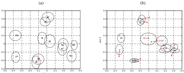
and 95% confidence interval). Results can be seen on figure 4.a. The average position of a
sound is indicated by a star. As expected, this position is close to the position in the
reference space which is labelled as a number. The ellipse represents the 95% confidence
location of this position.
The same computation was done using data obtained from the free sorting experiment and
gave the results represented on figure 4.b. It can be seen that sounds coordinates are
somewhat different from the reference ones. As an example, sound 27 is closer to sounds 3
and 6 than to sound 8, which was not true in the reference plane. For five sounds only (30, 3,
From this analysis, it can be thought that the dissimilarities obtained from the free sorting
experiment lead to a perceptual space slightly different from the one issued from the
pair-wised estimations.
6. DISCUSSION
In the case of this study, the averaged co-occurrence matrix did not provide a perfect
alternative to direct dissimilarities. As presented in figure 2, the two kinds of data were close
to each other for rather similar sounds only.
The key point is that, in a free sorting experiment, individual co-occurrence matrices only
contain 0 and 1 values. Inter-individual variability is thus necessary to obtain an averaged
matrix which can be considered as a dissimilarity one. Consider an extreme case in which
stimuli are grouped in three families by all subjects. The averaged co-occurrence matrix will
also contain 0 and 1 values only and the perceptual space will take the form of an equilateral
triangle in a plane. In such a situation, direct dissimilarity estimation may give more accurate
information, as it is possible that dissimilarities perceived between two of these groups will
be lower than those between each of these two groups and the third one. This information
will not appear in the results of the free-sorting task.
In some cases, such a small inter-individual variability can be expected: an example may be
an experiment in which very different sound sources are used. It is probable that all listeners
will group sounds together according to their sources. When the set of sounds is more
homogeneous, as in most sound quality applications, more various individual sorting data
are collected. It can then be expected that averaged data can be considered as dissimilarities,
at least for the closest sounds only, as it has been shown in this study. The inter-individual
variability occurring in a free-sorting experiment can be estimated from the corrected Rand
the accuracy of the perceptual space computed from a free sorting experiment to the range of
Rand Indexes computed between each pair of subjects. That could allow fixing some rules,
e.g. a maximum value of averaged Rand Index over which it cannot be recommended to
derive a perceptual space from the co-occurrence matrix.
Nevertheless, this limitation in the use of free-sorting experiments should not hide a very
useful application of this procedure. As confirmed by the first experiment of this study, it
can be used to reduce the number of stimuli, in cases where this number is too high to
conduct pair-wise dissimilarity ratings.
7. CONCLUSION
This study showed that a free sorting experiment can be very useful to reduce the number of
sound samples while keeping the main sounds features in the reduced set. That can be of a
great practical importance in sound quality applications.
It is also possible to directly build a perceptual space from the results of a free-sorting
experiment. But, as noted here, this space can be slightly different from the one computed
from direct evaluations of dissimilarities. It can be expected that the larger the dissimilarities
between sounds, the larger these differences will be, as inter-individual variability is
necessary to obtain almost continuous values when averaging free-sorting individual data.
This limitation should not hide one of the main advantages of a free sorting experiment: it
can involve a much larger number of samples than a paired comparison experiment. This
made it very suitable for industrial applications of studies related to sound quality.
For sound quality applications, a practical recommendation would be to include a large
number of sounds in the first set of stimuli presented to a jury. Thanks to a free-sorting
reduced set of sounds can be used in a pair-wise dissimilarity evaluation experiment in order
to build a reliable perceptual space.
REFERENCES
Barbot B., Lavandier C., Cheminée P. (2008) Perceptual representation of aircraft sounds, Applied Acoustics, 69, 1003-1016.
Bigand, E., Vieillard, S., Madurell, F., Marozeau, J., Dacquet, A. (2005). "Multidimensional scaling of emotional responses to music: the effect of musical expertise and of the
duration of excerpts", Cognition Emotion 19 (8), 1113-1139.
Börner, K. (2000) "Searching for the perfect match: A comparison of free sorting results for images by human subjects and by Latent Semantic Analysis", Information Visualisation 000, Symposium on Digital Libraries, London, England, 19-21July, pp. 192-197. Cox, T.F., Cox, M.A. (2001). Multidimensional scaling (Chapman & Hall, Boca Raton). Dubois D., Guastavino C., Maffiolo V. (2004). "The meaning of city noises: Investigating
sound quality in Paris (France)", J. Acoust. Soc. Am. 115, 2592.
Dubois ,D., Guastavino C., Raimbault, M. (2006). "A cognitive approach to urban soundscapes : using verbal data to access everyday life auditory categories" , Acta Acustica united with Acustica 92, 865-874.
Edwards J.A., Templeton A. (2005). "The structure of perceived qualities of situations", Eur. J. Soc. Psychol. 35, 705-723.
Falahee, M., MacRae, A. (1997). "Perceptual variation among drinking waters: the reliability of sorting and ranking data for multidimensional scaling," Food Qual. Prefer. 8 5/6, 389-394.
Faye P., Brémaud D., Durand Daubin M., Courcoux P., Giboreau A., Nicod H. (2004). "Perceptive free sorting and verbalization tasks with naive subjects: an alternative to descriptive mappings", Food Qual. Prefer. 15, 781-791.
Guastavino C. (2003). "Etude sémantique et acoustique de la perception des basses fréquences dans l'environnement sonore urbain" ("Semantic and acoustic study of low-frequency noises perception in urban sound environment"), Ph.D. dissertation , Université Paris 6 (available from http://jubil.upmc.fr/repons/portal/portal, date last viewed 6/18/10). Guyot, F., Catellengo, M., Fabre, B. (1997). "Etude de la catégorisation d'un corpus de bruits
cognition : de la perception au discours (Categorization and cognition, from perception to language), edited by D. Dubois (Kimé, Paris), pp. 41-58.
Houix, O., Lemaître, G., Misdariis, N., Susini, P. (2008). "Classification of everyday sounds: influence of the degree of sound source identification", J. Acoust. Soc. Am. 123, 3414. Hubert, L., Arabie, P. (1985). "Comparing partitions", J. Classif. 2, 193-218.
Kendall, R. A. & Carterette, E. C. (1991) "Perceptual scaling of simultaneous wind instrument timbres" Music Perception, 8, 369-404.
Lavandier, M., Meunier, S., Herzog, P. (2005) "Perceptual and physical evaluation of differences among a large panel of loudspeakers", Proc. Forum Acusticum 2005, (Budapest, Hungary).
Lemaitre, G., Susini, P.,Winsberg, S., B., McAdams, S. (2004). "A method to assess the ecological validity of laboratory-recorded car horn sounds", CFA/DAGA, Strasbourg, France.
Maffiolo, V. (1999)."Caractérisation sémantique et acoustique de la qualité sonore de
l'environnement urbain" ("Semantic and acoustic characterization of urban environmental sound quality") Ph.D. dissertation, Université du Maine, France
McAdams S., Winsberg S., Donnadieu S., De Soete G., Krimphoff J. (1995) "Perceptual scaling of synthesized musical timbres: common dimensions, specificities, and latent subject classes" , Psychological Research, 58, 177-192.
Montignies F., Parizet E. (2008) "Study of the perceptive space linked to dashboard tapping sounds", J. Acoust. Soc. Am. 123, 3298.
Parizet, E., Guyader, E., Nosulenko, V. (2007) "Analysis of car door closure sound quality", Applied Acoustics 69, 12-22.
Picard D., Dacremont C., Valentin D., Giboreau A. (2003). "Perceptual dimensions of tactile textures", Acta Psychol. 114, 165-184.
Rips, L.J. (1993). "Categories and resemblance," J. Exp. Psychol. – Gen. 122, 468-486. Saporta, G. (2006). "Probabilités, analyse des données et statistiques" ("Probability, data
analysis and statistics"), (Technip, Paris).
Thibaut, J.-P. (1997). "Similarité et catégorisation" ("Similarity and categorization") Ann. Psychol. 97, 701-736.
Tiest, W.M.B., Kappers, A.M.L. (2006). "Analysis of hatpic perception of materials by multidimensional scaling and physical measurements of roughness and compressibility", Acta Psychol. 121, 1-20.
Collected Figure Captions
Figure 1: dendrograms obtained from the three experiments. (a) : free sorting, 35 sounds.
(b) : free sorting, 12 sounds. (c) : paired comparison, 12 sounds. Groups of
sounds are labelled with letters.
Figure 2: comparison of dissimilarities obtained from the free sorting experiment and the
direct evaluation. Circles indicate pairs for which the two values are not different
in a significant way (p<0.05, Kruskal Wallis criterion).
Figure 3: MDS mappings of stimuli. Bold letters: from dissimilarity ratings. Italic letters:
from free sorting experiment.
Figure 4: MDS mappings of stimuli and application of the bootstrap technique. (a):
dissimilarity ratings, (b): free-sorting experiment. In both cases, the number
represents the average position of the sound, the ellipse the 95% confidence
interval. The star denotes the position of the sound in the reference space
11 12 20 21 14 18 29 30 19 1 4 17 2 3 6 5 27 23 7 8 13 15 16 33 9 10 28 22 34 35 24 31 32 25 26 0 0.5 1 1.5 2 2.5 (a) 06 03 16 13 27 08 30 18 09 28 26 32 0 0.5 1 1.5 (b) 16 13 30 18 09 28 26 32 27 08 06 03 0.2 0.4 0.6 0.8 (c) B D D B D B C C C A A A E E E F F F
Figure 1: dendrograms obtained from the three experiments (a): free sorting, 35 sounds, (b):
free sorting, 12 sounds and (c): dissimilarity evaluation, 12 sounds. Groups of sounds are
0.0 0.2 0.4 0.6 0.8 1.0 0.0 0.2 0.4 0.6 0.8 1.0
diss imilarities (free sorting)
d is s im il a ri ti e s ( p a ir -w is e d c o m p a ri s o n s )
Figure 2: comparison of dissimilarities obtained from the free sorting experiment and the
direct evaluation. Circles indicate pairs for which the two values are not different in a
-0.4 -0.3 -0.2 -0.1 0 0.1 0.2 0.3 0.4 -0.3 -0.2 -0.1 0 0.1 0.2 0.3 0.4 18 18 30 30 3 3 6 6 8 8 27 27 13 13 16 16 9 9 28 28 26 2632 32 axis 1 a x is 2
Figure 3: MDS mappings of stimuli (axes 1 and 2). Bold letters: from dissimilarity ratings.
(a) -0.5 -0.4 -0.3 -0.2 -0.1 0 0.1 0.2 0.3 0.4 -0.3 -0.2 -0.1 0 0.1 0.2 0.3 0.4 18 30 3 6 8 27 13 16 9 28 26 32 axis 1 a x is 2 (b)
Figure 4: MDS mappings of stimuli and application of the bootstrap technique. (a) :
dissimilarity ratings, (b) : free-sorting experiment. In both cases, the number represents the
average position of the sound, the ellipse the 95% confidence interval. The star denotes the
position of the sound in the reference space (dissimilarity ratings averaged over the whole
panel). -0.5 -0.4 -0.3 -0.2 -0.1 0 0.1 0.2 0.3 0.4 -0.3 -0.2 -0.1 0 0.1 0.2 0.3 0.4 18 30 3 6 8 27 13 16 9 28 2632 axis 1 a x is 2