Modélisation spatiale multiscalaire de la structure des communautés de poissons lacustres en relation avec les facteurs environnementaux littoraux
par
Anik Brind’Amour
Département des sciences biologiques Faculté des arts et des sciences
Thèse présentée à la faculté des études supérieures en vue de l’obtention du grade de
Philosophiœ Doctor(Ph.D.) en sciences biologiques
Avril 2005
3f1
o
uS!
;035
oo3
dl1
de Montréal
Dïrection des bibliothèques
AVIS
L’auteur a autorisé l’Université de Montréal à reproduire et diffuser, en totalité ou en partie, par quelque moyen que ce soit et sur quelque support que ce soit, et exclusivement à des fins non lucratives d’enseignement et de recherche, des copies de ce mémoire ou de cette thèse.
L’auteur et les coauteurs le cas échéant conservent la propriété du droit d’auteur et des droits moraux qui protègent ce document. Ni la thèse ou le mémoire, ni des extraits substantiels de ce document, ne doivent être imprimés ou autrement reproduits sans l’autorisation de l’auteur.
Afin de se conformer à la Loi canadienne sur la protection des
renseignements personnels, quelques formulaires secondaires, coordonnées ou signatures intégrées au texte ont pu être enlevés de ce document. Bien que cela ait pu affecter la pagination, il n’y a aucun contenu manquant. NOTICE
The author of this thesis or dissertation has granted a nonexclusive license allowing Université de Montréal to reproduce and publish the document, in
partor in whole, and in any format, solely for noncommercial educational and
research purposes.
The author and co-authors ifapplicable retain copyright ownership and moral
rights in this document. Neither the whoTe thesis or dissertation, nor
substantial extracts from it, may be printed or otherwise reproduced without the author’s permission.
In compliance with the Canadian Privacy Act some supporting forms, contact information or signatures may have been removed from the document. While this may affect the document page count, t does flot represent any loss of content from the document.
Université de Montréal faculté des études supérieures
Cette thèse intitulée
Modélisation spatiale multiscalaire de la structure des communautés de poissons lacustres en relation avec les facteurs environnementaux littoraux
Présentée par Mik Brind’Arnour
A été évaluée par un jury composé des personnes suivantes:
André Bouchard président-rapporteur Daniel Boisclair directeur de recherche Nicolas Lamouroux examinateur externe Frédéric Guichard Examinateur externe Jacques Bélair
SOMMAIRE
Les communautés lacustres de poissons littoraux sont exposées à un environnement comprenant une grande hétérogénéité structurale à plusieurs échelles spatiales, variant du millimètre à une centaine de mètres. Par conséquent, les interactions entre les poissons et l’environnement peuvent avoir lieu à différentes échelles spatiales. Des études récentes ont montré que la validité des modèles d’habitats de poissons pouvait être fortement compromise lorsque la structure spatiale de la zone littorale n’était pas intégrée à ces modèles.
L’objectif principal de ma thèse était de modéliser la distribution spatiale multiscalaire des communautés de poissons lacustres en relation avec les facteurs environnementaux. Or, l’étude de l’impact de la structuration spatiale de la zone littorale des lacs sur les communautés de poissons nécessite une technique d’échantillonnage qui soit continue dans l’espace. De nature méthodologique, le Chapitre 1 a servi de base aux trois autres chapitres en montrant la validité du recensement visuel comme méthode d’échantillonnage dans la zone littorale. La seine de rivage, une méthode d’échantillonnage traditionnelle, a été utilisée à titre comparatif. Des descripteurs de la communauté de poissons comparés, la densité totale et la biomasse totale furent visuellement sous-estimées en comparaison avec la seine. Cette divergence entre les deux méthodes fut principalement attribuable à la stratégie d’échantillonnage employée lors du comptage des individus.
La modélisation fut effectuée en deux temps, à l’aide d’une approche multiscalaire, c’est-à-dire en modifiant les attributs relatifs à l’échelle d’analyse spatiale. Dans un premier temps, Futilisation d’une méthode «analyse statistique
Iv
tenant explicitement compte de la distance entre les unités d’échantillonnage a permis d’observer que les espèces littorales présentaient une variété de patrons de distribution s’échelonnant sur des distances géographiques variant de 100 m à plus de 2 km. Les patrons de distribution associés aux différentes échelles spatiales furent corrélés à différentes variables environnementales, suggérant ainsi la présence de processus écologiques structurant la communauté de poissons spécifique à certaines échelles spatiales (Chapitre 2). Les résultats de ce chapitre ont permis d’émettre certaines hypothèses portantsur la distribution spatiale hiérarchisée des espèces et de leur relation fonctionnelle avec l’environnement. Ces hypothèses furent vérifiées au Chapitre 3, dans lequel nous avons observé si les traits morphologiques et comportementaux des espèces influençaient leur type de patron de distribution spatiale. L’association de certains traits biologiques a permis de regrouper les espèces en trois groupes fonctionnels associés à la position de la bouche et au niveau où elles se nourrissent dans la colonne d’eau (c.-à-d. ségrégation verticale). Les groupes fonctionnels présentaient des différences en ce qui concerne leur association avec différents types d’habitats, suggérant ainsi une ségrégation à la fois verticale et horizontale (entre habitats). L’interprétation de ce chapitre est toutefois mitigée en raison des faibles corrélations obtenues entre les traits et l’environnement.
La diversité des patrons de distribution des espèces sur plusieurs échelles géographiques suggérait notamment l’importance des interactions entre les caractéristiques environnementales et le contexte spatial dans lequel les espèces évoluent. Dans un deuxième temps, cette suggestion fut vérifiée par l’étude de l’impact de la modification du grain de l’échelle d’analyse (c.-à-d. l’utilisation de
différentes tailles d’unités d’analyse) sur la performance des modèles d’habitats (Chapitre 4). Trois tailles d’unités d’analyses, chacune caractérisée par un type de contrainte spatiale, ont ainsi été comparées. La taille de l’unité d’analyse, représentée par le regroupement de sites contigus caractérisés par des variables environnementales similaires (c.-à-d. en tache), a fourni les modèles les plus performants. De plus, l’intégration de variables décrivant l’arrangement spatial des habitats a permis d’observer que les poissons ne sont pas influencés que par les caractéristiques locales, ils sont également influencés par les caractéristiques présentes dans les habitats voisins.
Soulignant la présence de groupes fonctionnels associés à différentes échelles spatiales et l’importance des taches d’habitats dans la structure des communautés de poissons, les résultats de cette thèse suggèrent l’attribution d’une identité et d’une valeur écologique à la variété des habitats, définissant ainsi la zone littorale comme une « diversité fonctionnelle > d’habitats. En regard à la problématique actuelle
portant sur la conservation des habitats dans la zone littorale des lacs, les résultats suggèrent que la taille d’un habitat ne saurait représenter le seul critère nécessaire au maintien de cette diversité fonctionnelle. Les interactions entre la taille des taches d’habitat, la distribution spatiale et les caractéristiques environnementales (intrinsèques et extrinsèques) associées à ces taches représenteraient autant de critères à tenir en compte dans l’élaboration des plans de conservation, afin d’assurer le maintien de la diversité des communautés littorales.
Mots clés communauté lacustre, distribution spatiale, facteurs environnementaux, groupe fonctionnel, habitat, modèles prédictifs, multiscalaire, poissons, zone littorale.
VI
S UMMARY
Fish communities of the littoral zone of lakes are exposed to a structurally complex environment over multiple spatial scales ranging from millimeters to hundreds of meters. Consequently, the interactions between littoral fish communities and their habitat may take place at different spatial scales. Recent papers showed that when ignored, that scale-dependency between fish communities and their habitat could jeopardize the validity of species habitat models.
This thesis had for main objective to model the spatial distribution of littoral fish communities in lakes in relation to environmental factors. The multiscale approach was used in respect to variations in the scale of the spatial analyses. This was done in two steps. At first, we used a statistical approach that took in consideration the distance between the sampling units. Using this approach we observed that the fish community exhibited scale-dependent variability that we grouped in four categories (or submodels), at spatial scales ranging from <100 m to 2 km. These submodels were associated with specific environmental variables, suggesting the presence of scale-dependent ecological processes within the lake (Chapter 2). Results from this chapter allowed us to establish several hypotheses concerning the hierarchical spatial distribution of fish species in relation to their functional relationship with the environment. These hypotheses were verified in chapter 3 in which we tested if species behavioural and morphological traits determined their spatial distribution in lakes. We observed concordance among the species traits suggesting the presence of three functional groups of species according
to the position of the mouth and the location of the flsh in the water column (superior surface, terminal-mid-water, and inferior-benthic). Correlations between the groups of species traist and the environment suggested the presence of habitat segregation along the vertical (water column) and horizontal (habitats) dimensions. However, a constraint interpretation of these resuits was doue because of the low traits environment correlations observed.
In the second step of the multiscale modelling, we tested the impact of the modification of the size of the analytical unit on the performance of fish habitat models (Chapter 4). Analytical units of three sizes, caracterised by different groupings of the sampling sites, were compared. Models developed with analytical unitsrepresented by the grouping of contiguous sampling sites with similar environmental characteristics (i.e. in habitat patch), displayed the highest predictive power. Integration of variables describing the spatial arrangement of habitat within the littoral zone of the lake showed that fish species may flot be determined only by the environmental characteristics found within this site but also by conditions found in surrounding locations.
The mulstiscale modeling of the spatial distribution of littoral fish communities in lakes, required a spatially continuous sampling technique. Chapter 1 rooted the other three chapters by validating and establishing the limits in which the visual census tecimique could be used in this thesis.
Underlying the presence of functional groups associated with multiple spatial scales and the importance of habitat patches in the structure of littoral fish communities, the results from this thesis suggest to assignate an ecological value to
VIII
the variety of habitat patches, thereby characterising the littoral zone of a “functional diversity” of habitats. From a conservation point of view, the resuits also suggest that the size of habitat patches is not the only criteria on which preservation of functional diversity of the littoral zone is based. Interactions between the size of the habitat patch, spatial arrangement of the patches, and the environmental conditions (intrinsic and extrinsic) associated with these patches likely represent significant criteria to maintain the diversity of fish communities in lakes.
Keywords: fish con]munity, littoral zone, lake, multiscale. spatial patterns, habitat, patch, predictive models, functional groups, environmental factors.
TABLE DES MATIÈRES
SoMMAIRE III
SuMMARY VI
TABLE DES MATIÈRES IX
LISTE DES TABLEAUX XIII
LISTE DES FIGURES XVI
REMERCIEMENTS XXI
INTRODUCTION GÉNÉRALE 1
PROBLÉMATIQUE 1
SÉLECFI0N D’HABITAT ET NICHES ÉCOLOGIQUES 2
PATRoNs SPATIAUX ET PROCESSUS ÉCOLOGIQUES MULTISCALAIRES 4
STRUCTURE DE LA ZONE LITTORALE DES LACS 6
OBJEcfIFS DE RECHERCHE 8
CHAPITRE 1 COMPARISON BETWEEN TWO SAMPLING METHODS
TO EVALUATE THE STRUCTURE 0F FISH COMMUNITIES IN THE
LITTORAL ZONE 0F A LAURENTIAN LAKE 12
ABsTRACT 12
INTRODUCTIoN 13
MATERIALs AND METHODS 15
Study lake 15 Sampling procedure.s 15 Computations 21 Statistical analyses 23 REsuLTS 25 Habitat classification 25 Cornmunity descriptors 26 DISCUSSION 30
X
CHAPITRE 2 MULTISCALE SPATIAL DISTRIBUTION 0F A LITTORAL FISH COMMUNITY IN RELATION TO ENVIRONMENTAL VARIABLES 36
ABSTRACT 36
INTRODUCTION 37
METH0D5 39
Study lake 39
Sampling procedure 40
Fish community sampling 41
Computations 43
Environmental variables 44
Statistical analyses 46
RESULTS 48
Classifïcation of spatial scales 50
Multiscale patterns 50 DIscussIoN 64 Spatially-structured habitats 65 Temporal scale 69 Species specialization 70 APPENDIx A 75
CHAPITRE 3 MULTI-SCALE ASSESSMENT 0F THE FUNCTIONAL RELATIONSHIPS BETWEEN SPECIES TRAITS AND THE
ENVIRONMENTAL CONDITIONS FOR LITTORAL fISH COMMUNITIES7$
ABSTRACT 7$
INTRODUcTION $0
MATERIALs AND METHODS $2
Study lakes 82
Sampling procedure 83
Methodological framework $4
REsuLTs 93
Associations of species traits 94
Species traits and environmental variables 97
Functional feeding groups .102
Multiscale habitat use 104
Implications in habitat modeling 107
Conclusion 10$
APPENDIx A 110
CHAPITRE 4 EFFECT 0F THE SPATIAL ARRANGEMENT 0f HABITAT PATCHES ON THE DEVELOPMENT 0F FISH HABITAT
MODELS IN THE LITTORAL ZONE 0F A CANADIAN SHIELD LAKE...11$
ABsTRAcT 11$
INTRODUCTION 119
MATERIALs AND METHODS 121
Study lake 121
Sampling procedure 122
Fish community descriptors 123
Computations 124
Environmental characteristics 125
Data analysis 127
RE5uLT5 131
Clustering of sampling sites 132
Sampling-site approach 134
Constant-multiple approach 135
Habitat-patch approach 137
Fish-habitat models 137
DIscussIoN 14$
Size of analytical units 149
Why use habitat patches9 150
Influence of extrinsic variables 151
Sized-structured patchiness 153
Conclusion and perspective 155
XII
CONCLUSION GÉNÉRALE .162
RECENSEMENT VISUEL DES COMMUNAUTÉS DE POISSONS 163
STRuCTuRE SPATIALE HIÉRARCHISÉE DES COMMUNAUTÉS LITTORALES 164
SÉGRÉGATION FONCTIONNELLE DES HABITATS 165
LA TACHE: UNE UNITE D’ANALYSE APPROPRIÉE 167
CONSERVATION DES HABITATS LITTORAUX LACUSTRES 169
STRATÉGIES D’ÉCHANTILLONNAGE 169
ORIGINALITÉ 170
PERSPECTIVES ET AMÉLIORATIONS 170
LISTE DES TABLEAUX
Chapitre 1
Table 1.1 Description of the four environmental characteristics. Macrophyte density was estimated by the individual per m2 and the different types of substrate
were expressed as binary variables 17
Table 1.2 Size range, measured with a precision equal to ± 2.5 mm, for each
species sampled in the community. The asterisk identifies the species sampled with the seine and the visual surveys. Common names are in parenthesis 22 Chapitre 2
Table 2.1 Species size classes used in the text. The species marked with an asterisk was excluded from the analysis because its total abundance was less than 1%. Numbers in parentheses indicate the percentage (%) of fish observed by size
class 43
Table 2.2 Numerical resolutions and codes for the environmental variables
observed at each site 45
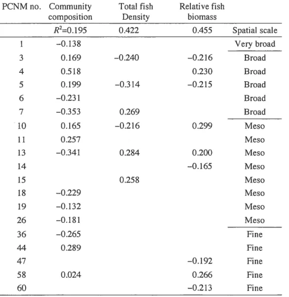
Table 2.3 Regression/canonical coefficients for standardized variables of fish community descriptors detected at different spatial scales in June. Column headings: coefficients of determination
(R2)
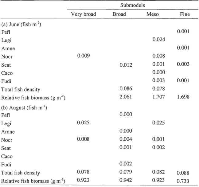
for the whole spatial model 52 Table 2.4 Species scores on the first canonical axis of each spatial scale submodel for the months of June and August. : Species which are markedly contributing to a given scale. No significant relationship was found between the community composition and the fine spatial scale in August 53 Table 2.5 Median values of the fish community descriptors for the four submodels (a) for the month of June and (b) the month of August 54 Table 2.6 June: standardized coefficients (b) of environmental variables which explained significant components of the spatial patterns (PCNM models) of the littoral fish community descriptors at four different spatial scales. Sec Table 2 for theXIV
environrnental variable codes. Column headings: coefficients of determination (R2) of the rnodels.* O.Ol<p 0.05:’
O.00l<p
0.01;’ p 0.001 55 Table 2.7 Regression!canonical coefficients for standardized variables of fish community descriptors detected at different spatial scales in August. Column headings: coefficients of determination (R2) for the whole spatial model 62 Table 2.8 August: standardized coefficients (b) of environmental variables which explained significant components of the spatial patterns (PCNM models) of the littoral fish community descriptors at four different spatial scales. See Table 2 for the environmental variable codes. Column headings: coefficients of determination (R2) of the models.* 0.0l<p 0.05; 0.001<p 0.0l;***p 0.001 63 Table 2.9 Habitat classification based on the environmental variables associatedwith the four spatial subrnodels 66
Chapitre 3
Table 3.1 Species size classes and composition (presence-absence) in Lac Drouin
and Lac Paré 86
Table 3.2 Description of the species biological and behavioral traits used in this study. Code numbers for the species traits are in brackets $8 Table 3.3 Codes and numerical resolutions ofthe environmental variables $9 Table 3.4 Classification ofthe fish species pertaining to each functional group in Lac Drouin and Lac Paré, obtained by PCA on the species behavioral and morphological trait matrices (i.e. matrix B). A : G51. Â: G1*, D : G2, O:
Table 3.5 Summary of the colTelation values between the three groups (G) of species traits and the environment in the two lakes at very broad and broad spatial
Chapitre 4
Table 4.1 Intrinsic and extrinsic (Spat) environmental variables that were respectively either sampled or computed at each sampling site for the sampling-site (S), the constant-multiple (C), or the habitat-patch (P) approaches. ‘: Percent of
presence in all the sampling sites 126
Table 4.2 EnvironmentaÏ characteristics for each type of habitat display in the
littoral zone of Lac Drouin 133
Table 4.3 Summary of the variability of the community descriptors found for the constant-multiple approach among the six groupings of sampling sites 136 Table 4.4 Sampling-site models developed for the total fish density (TFD). the relative biomass (RB) and the size classes of fish (SC) (n=90) and the relative contributions of the intrinsic and extrinsic variables. ***: p 0.001 13$ Table 4.5 Summary (mean R2 and standard deviation; S.D.) of the constant-multiple models developed for the total fish density (TFD). the relative biomass (RB) and the size classes of fish (SÇ). *: Adjusted R2 141 Table 4.6 Habitat-patch empirical models developed for the total fish density (TFD). the relative biomass (RB) and the size classes of fish (SC). Variable codes
are defined in Table 1. ***: p 0.001 144
Table 4.7 Summary (R2, standard deviation; S.D., percentile; perc, minimum; mm, and maximum; max) of the habitat-patch models using obtained by habitat patches randomly distributed in the littoral zone of the lake. R2 for the habitat-patch models obtained with patches based on environmental characteristics are found in
xv’
LISTE DES FIGURES
Introduction générale
Figure 1.1 Schéma représentant la réponse d’une espèce face à (A) un gradient environnemental et (B) deux gradients environnementaux. [adapté de Giller 1984 et
Choler 20021 3
Figure 1.2 Représentation graphique du concept d’échelle spatiale définit par ses
trois dimensions. [adaptation Dungan et cou. 2002]
5
Figure 1.3 Schématisation de la structure de la présente thèse en quatre
chapitres 9
Chapitre 1
Figure 1.1 Location of the ten sites classified by the three classes of habitat (H) at Lake Drouin (Quebec). Black squares along the lake contour represent houses and
cottages 16
Chapitre 2
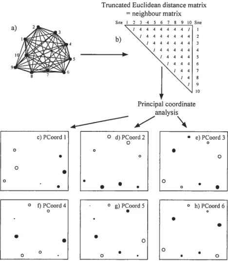
Figure 2.1 Map of Lake Drouin (Lanaudière, Québec). Black dots represent the 90 sampling sites in the littoral zone of the lake 40 Figure 2.2 PCNM variables around a fictitious structure forming a loop. (a) Sites localized on the map. (b) Neighbor matrix. Distances between neighboring sites (heavy unes in a) are written in the neighbor matrix in b; these distances are equat to 1 in the example. Distances between non-adjacent sites (light lines in a) are replaced by 4 times the maximum value (max=1 in the example, 4 max=4). (e-h) The successive PCNMs are presented by bubbles on the map of the sites: Positive values
are filled, negative values are empty 47
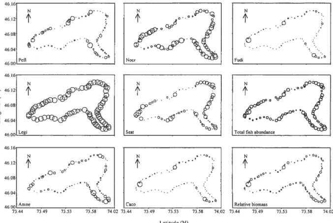
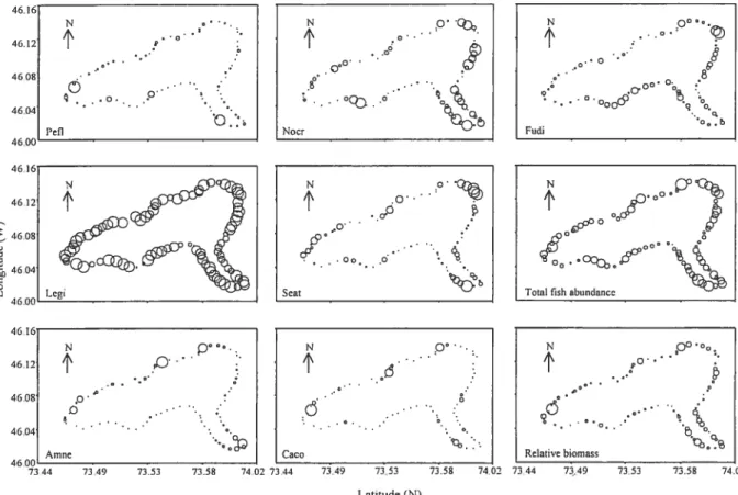
Figure 2.3 Map of Lake Drouin showing the observed values of the fish community descriptors (A) for the month of June and (B) the month of August. The size of the bubbles is proportional to the observed values 49
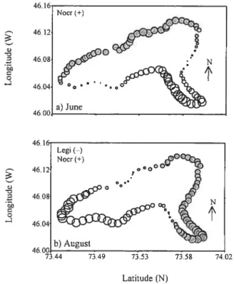
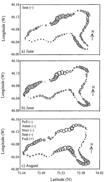
Figure 2.4 Map of Lake Drouin showing (a) the forecasted values of the community composition in June, and (b) the three fish community descriptors in August at the very broad scale ( 2 km). The size of the bubbles is proportional to the forecasted values. The species marked with (+) and
t—)
are abundant in the filled and empty bubbles respectively; see Table 4 for details. Species codes are given in Table1 51
Figure 2.5 Map of Lake Drouin showing (a) the forecasted values of the community composition, and the total fish density, (b) relative fish biomass in June. (c) The community composition, the relative fish biomass and the total fish density in August at the broad scale (500-1000 m). The size of the bubbles is proportional to the forecasted values. The species marked with (+) and
(—)
are abundant in the filled and empty bubbles respectively; see Table 4 for details. Species codes are given in Table 57 Figure 2.6 Map of Lake Drouin showing (a) the forecasted values of the community composition and the total fish density, and (b) relative fish biornass in June. (c) The three fish community descriptors in August at the meso scale (300-500 m). The size of the bubbles is proportional to the forecasted values. The species marked with (+) and(—)
are abundant in the filled and empty bubbles respectively; see Table 4 for details. Species codes are given in Table 1 5$ Figure 2.7 Map of Lake Drouin showing (a) the forecasted values of the community composition and the relative fish biomass in lune . (b) The total fish density and the relative fisli biomass in August at the fine scale (<100 m). The size of the bubbles is proportional to the forecasted values. The species marked with (+) and(—)
are abundant in the filled and empty bubbles respectively; see Table 4 for details.Species codes are given inTable 1 60
Figure 2.8 Schematic structure of three functional groups based upon the associations of the species with different ranges of spatial scales 71
XVIII
Chapitre 3
Figure 3.1 Bathymetric maps of the two study lakes on the Canadian Shield in
Québec (Canada) $3
Figure 3.2 Schematic illustration of the fourth-corner statistical analysis used in our study. In matrix C, the variables are predicted values from multiple regressions
(see Materials and methods) $5
Figure 3.3 Proportion of the total variance of the species traits explained by the environmental variables at the four spatial scales in Lac Drouin (circles) and Lac Paré
(squares) 93
Figure 3.4 PCA ordinations showing the groups of species traits (G) for (A) Lac Drouin at very broad spatial scale, (B) Lac Drouin at broad spatial scale, (C) Lac Paré at very broad spatial scale, and (D) Lac Paré at broad spatial scale. Codes for the functional groups are found in Table 2. PCA were done using species traits that were significantly correlated to the environrnent, therefore the numbers indicating the
species traits may vary arnong the four figures 94
Figure 3.5 Conelations between species traits and environmental variables at very broad spatial scale in Lac Drouin. Significant positive correlations are in dark grey, significant negative correlations in light grey, and non-significant correlations in white. Codes for the environmental variables are described in Table 2 9$ Figure 3.6 Correlations between species traits and enviromnental variables at very broad spatial scale in Lac Paré. Significant positive correlations are in dark grey, significant negative correlations in light grey, and non-significant correlations in white. Codes for the environmental variables are described in Table 2 99 Figure 3.7 Correlations between species traits and environrnental variables at broad spatial scale in Lac Drouin. Significant positive correlations are in dark grey, significant negative correlations in light grey, and non-significant conelations in white. Codes for the environmental variables are described in Table 2 100
Figure 3.8 Correlations between species traits and environmental variables at broad spatial scale in Lac Paré. Significant positive correlations are in dark grey, significant negative correlations in light grey, and non-significant conelations in white. Codes for the enviromuental variables are described in Table 2 101 Figure 3.9 Schernatic model of the spatial distribution of littoral fish species from Lac Drouin according to their biological and behavioral traits, across four spatial scales symbolized by the circle surface areas. The fish heads represent the three functional groups of species. The lengths refer to the shore lengths and the percentages are the portions of the perimeter of the lake covered by a habitat patch at
the given scale 107
Chapitre 4
Figure 4.1 Map of Lac Drouin (Lanaudière. Québec). Black dots represent the 90
sampling sites in the littoral zone of the lake 122
Figure 4.2 Schematic description of the three approaches used in this study, the sampling-site approach (A), the constant-multiple approach (B), and the habitat-patch
approach (C) 127
Figure 4.3 Sites scores on the second and third dimensions (12.6% and 8.7% of variance explained respectively) for the 90 sites located on the littoral zone of Lac Drouin. The symbols represent the six clusters identifïed by Ward’s cluster
analysis 132
Figure 4.4 Spatial structure of the littoral zone of Lac Drouin. Codes for clusters
are defined in Table 1 134
Figure 4.5 Ordination from the RDA showing the relationships between fish species and environmental variables for the habitat-patch model. Only the first dimension of each model was significant and accounted for 58.1% of the fish
community variability 139
Figure 4.6 Relative contributions of the local variables (A) and the spatial arrangement variables (B) to the three types of models 143
xx
Figure 4.7 Ordination from the RDA showing the relationships between fisli species and environmental variables for the sampling-site approach. Only the first dimension was significant and accounted 64.5% of the fisli communityREMERCIEMENTS
D’abord merci à mon directeur de recherche, Daniel Boisclair qui m’a fait confiance dès le début et qui m’a laissé une grande liberté tout au long de la réalisation de ce projet. J’ai beaucoup bénéficié de son expérience à plusieurs niveaux, notamment j’ai su développer un esprit critique, apprendre l’importance de bien synthétiser les connaissances tant sur le plan oral qu’écrit et développer l’affirmation de mes idées à l’aide d’arguments scientifiques. Également merci pour son appui financier.
Merci à Pierre Legendre pour sa rigueur scientifique et son engouement contagieux pour les statistiques... multivariées. Mon petit « stage d’hybridation» de
fin de parcours au sein de son laboratoire m’a été extrêmement bénéfique, tant sur le plan professionnel que personnel... Suite aux multiples discussions, je comprends désormais d’où provient l’appellation jeu de données!
Je tiens à remercier les membres du jury dont les commentaires ont su apporter de nouvelles perspectives d’analyse et d’interprétation de la thèse, ce qui en a grandement amélioré le contenu et qui m’a permis de pousser davantage ma réflexion.
Ce projet de doctorat n’aurait pas vu le jour sans le soutien boursier de deux principaux organismes, le CRSNG et le fQRNT, qui m’ont libéré d’un souci financier pour la majeure partie de mon doctorat. Les supports financiers du GRIL et du Département des sciences biologiques m’ont également permis de participer et
XXII
d’assister à plusieurs congrès dont les échanges et les rencontres ont été bénifiques à l’avancement de cette thèse.
Un merci spécial aux collègues de dîner, c’est-à-dire à la gang de physiologie animale, pour les moments de détente et les nombreuses discussions. Merci aussi aux collègues et ex-collègues du labo Boisclair: Eva Enders, Guillaume Guénard, Jean Christophe Guay, Judith Bouchard, et aux multiples assistants de terrain avec qui j’ai eu bien du plaisir à échantillonner. De même, merci aux collègues du labo Legendre: Marie-Ève Ouellet, Sébastien Durant, Stéphane Dray, Pedro Peres-Neto, Guillaume Blanchet.
Merci au personnel de la station de biologie des Laurentides, au personnel de la bibliothèque et au personnel du département. Leur travail personnalisé et leur gentillesse ont grandement facilité et enjolivé mon quotidien sur le terrain et au PMV.
Merci au GRIL, qui grâce aux diverses activités (symposium, conférences du midi) j’ai pu élargir mon champ de connaissances et rencontrer plusieurs chercheurs. Spécialement merci à Claudette... une magicienne... qui a su faire disparaître bien des tracas administratifs et financiers.
Merci à ma famille, spécialement à mes parents, ma mère Pierrette, mon père Jean-Pierre et à Carole, pour leur soutien, leur générosité et leurs encouragements tout au long de mes études. Merci à mes soeurs Marie-Pierre et Martine et à ma grande famille élargie... Un merci spécial à mon oncle Royal avec qui j’ai appris que la pêche était une belle histoire de patience!
Merci aux amitiés de longue date, notamment Éric pour son écoute, sa générosité et surtout sa grandeur d’âme... Merci Max pour tes corrections et nos discussions de colocs! Aux amitiés développées au court de mon doctorat, notamment Chantai avec qui les discussions professionnelles et personnelles furent toujours très enrichissantes.
Un merci particulier à Nicolas... nos chemins se sont longuement croisés etje garde un précieux souvenir de ta présence et de ton soutien tout au long de cette traversée commune. Également merci à Mme Léger et M Bourgoin pottr leur grande générosité à bien des égards.
Musicalement merci à plusieurs auteurs-compositeurs pour leurs merveilleuses mélodies qui m’ont accompagnées tout au long de ma rédaction... Éric Satie, Ludwig van Beethoven, Leonard Cohen, Serge Gainsbourg, Claude Péloquin, Lhassa Desela, Alanis Morrissette et j’en passe...
« Tise scaks chosenfor analysis are stiil arbftrwy, however : they tend to reflect
hierarchies ofspatial xales tisai are based on osa own perceptions ofnature.
luit
because these panicular scaks scan ‘flght’ to us Li no
assurance
tisai they are appropflate toflsh,barnacles,
anoks, cattie, or birds.(Wiens,
1989)J-Introduction générale 1
PROBLÉMATIQUE
L’aménagement grandissant des zones riveraines des lacs entraîne la modification d’éléments riverains et littoraux qui peut avoir des répercussions importantes sur l’habitat du poisson. Au Québec, l’accroissement des aménagements riverains des lacs s’observe depuis une quarantaine d’années. Ces perturbations se concentrent principalement dans les régions les plus peuplées du Québec méridional (Gouvernement du Québec 2004). Parmi les modifications littorales, la substitution d’habitats hautement productifs caractérisés par des structures comportant une grande hétérogénéité structurelle (p. ex. troncs d’arbres morts et bancs de macrophytes), par des habitats de productivité réduite (p. ex. plages de sable) est caractéristique de nombreux lacs aménagés (Christensen et colI. 1996, Radomski et Goeman 2001). Plusieurs travaux ont identifié la perte d’habitats aquatiques comme étant une des causes principales menaçant la conservation des populations et des communautés de poissons des lacs (Evans et cou. 1987, Richter et coll. 1997). En effet, l’altération des habitats littoraux des poissons peut avoir d’importantes conséquences sur la structure des communautés de poissons, puisque ces habitats sont fortement impliqués dans l’organisation des écosystèmes lacustres (Wetzel 1990, Schiemer et Zalewski 1992). De même, de nombreuses espèces s’y retrouvent pour une ou plusieurs parties de leur vie, puisque la zone littorale assure un refuge contre les prédateurs (Mittelbach 1981, Tabor et Wurtsbaugh 1991, Gauthier et col!. 1997), fournit des aires d’alimentation (Werner et colI. 1983, Diehl 1993) et des aires de reproduction (Gafny et cou. 1992).
SÉLECTIoN D’ HABITAT ET NICHES ÉCOLOGIQUES
L’habitat d’un organisme peut se définir comme un espace (physique. chimique et biologique) associé à certaines structures et fonctions nécessaires à l’accomplissement du cycle de vie et au maintien de la population (Hayes et col!. 1996). Dans ce contexte, tous les habitats d’un écosystème aquatique ne sont pas également adéquats pour toutes les espèces à tous les stades de leur vie. La convenance de ces habitats peut varier selon les facteurs environnementaux (abiotiques et biotiques) et les échelles temporelles ou spatiales qui y sont associés (Eckmann 1991, Gaudreau et BoiscÏair 1998, Fréon et Misund 1999, Gaudreau et Boisclair 2000).
L’importance des facteurs environnementaux dans la sélection d’habitat a été théoriquement développée par le concept de niche écologique. Le terme de niche écologique fut introduit très tôt par Grinnell (1917). Selon cet auteur, la niche d’un organisme représentait tous les sites dont la combinaison de facteurs environnementaux permettait à l’organisme de survivre. Par la suite, Elton (1927) définit la niche comme étant la place qu’un organisme occupe dans un environnement biotique, c’est-à-dire en terme de relation fonctionnelle avec sa nourriture et ses ennemis. En prolongement de la notion de Grinnell, Hutchinson (1958) favorise une approche multidimensionnelle au concept de niche écologique, qu’il considère comme une gamme de variables environnementales (physique, chimique et biotique) pour lesquelles une espèce s’est adaptée. Cette adaptation se traduit notamment par une performance accrue (p. ex. forte abondance) à certains sites. Dans cette définition, chaque variable peut être considérée individuellement comme un gradient
Introduction générale 3 au long duquel l’abondance d’une espèce varie (Figure I.1A). Une espèce peut répondre à plusieurs gradients environnementaux qui définissent ainsi sa niche écologique (Figure I.1B). De nos jours, le concept de niche écologique évolue dans un contexte de contrôle multiple où la sélection d’habitat par une espèce est influencée par plusieurs facteurs environnementaux (ou ressources, sensu Magnuson et col!. 1979) pouvant opérer à différentes échelles spatiales et temporelles (Rabeni et Sowa 1996, Jackson et coll. 2001). Par ailleurs, l’étude des patrons spatiaux générés par la sélection d’habitat par les espèces et l’application de ces connaissances dans un contexte prédictif d’élaboration de modèles d’utilisation d’habitat, représente un des principaux buts de l’écologie des communautés (Menge et Olson 1990).
B
Q Q
-Q
Habitat favorable Habitat peu favorable
Figure 1.1 Schéma représentant la réponse d’une espèce face à (A) un gradient environnemental et (B) deux gradients environnementaux. [adapté de Giller 1984 et Choler 2002].
PATRONS SPATIAUX ET PROCESSUS ÉCOLOGIQUES MULTISCALAIRES
Définis comme étant une configuration ou un arrangement spatial des
éléments d’un écosystème, les patrons spatiaux désignent une caractéristique présente
dans pratiquement tous les écosystèmes naturels (Taylor et coll. 197$). Les plantes,
A
les animaux et même les variables physiques de l’environnement (p. ex. roches) forment des agrégations pour lesquelles divers patrons de distribution spatiale peuvent être observés (Legendre et Fortin 1989). Ces patrons de distribution spatiale, tant des éléments biotiques que des éléments abiotiques sont contrôlés par divers processus écologiques qui opèrent sur plusieurs échelles spatiales et temporelles. Notre compréhension des processus écologiques générant les patrons de distribution spatiale des espèces repose notamment sur notre capacité d’établir la correspondance entre les échelles de variations biologiques auxquelles se produisent les interactions spécifiques (p. ex. compétition, prédation) et les échelles de variations environnementales qui déterminent les relations entre les espèces et leur environnement (Levin 1999). Or, selon Pascual and Ellner (2000) le couplage de ces échelles de variations est très difficile à obtenir puisque les interactions entre ces dernières varient rarement de façon linéaire. Par exemple, la distribution spatiale d’une espèce peut être influencée par des conditions environnementales (p. ex. degré d’exposition au vent) opérant à des échelles spatiales très larges et présentant un pouvoir prédictif élevé. Cette même espèce peut être aussi influencée par des interactions biologiques (p. ex. prédation) opérant généralement à des échelles spatiales plus fines (Crowder et Cooper 1982) et générant un faible pouvoir prédictif lorsque ces modèles sont basés exclusivement sur des caractéristiques environnmentaÏes.
Notre perception de l’importance relative d’un ensemble de caractéristiques environnementales expliquant la distribution des espèces d’une communauté, varie donc en fonction des échelles spatiale et temporelle auxquelles ces relations sont
Introduction générale 5 analysées (Syms 1995). L’étude des patrons spatiaux à l’aide d’une approche multiscalaire, c’est-à-dire à différentes échelles spatiales et temporelles d’analyse, représente un outil essentiel pour comprendre les processus écologiques sous-jacents à la distribution spatiale des espèces et pour déterminer les impacts de ces processus écologiques sur la structure des communautés (p. ex. assemblages d’espèces, structure en taille; Wiens 1976, Menge et Olson 1990).
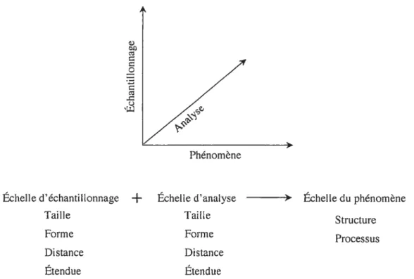
Dans cette présente thèse, le concept « d’échelle spatiale » est utilisé dans le sens récemment définit par Dungan et coll. (2002). L’échelle spatiale d’une étude repose sur trois dimensions s l’échelle d’échantillonnage (ou d’observation), l’échelle d’analyse statistique et l’échelle des phénomènes écologiques (Figure 1.2).
D
Q
Échelle d’échantillonnage + Échelle d’analyse > Échelle du phénomène
Taille Taille Structure
Forme Forme Processus
Distance Distance
Étendue Étendue
Figure 1.2 Représentation graphique du concept d’échelle spatiale définit par ses trois dimensions. [adapté de Dungan et colI. 20021.
Les deux premières échelles sont caractérisées par quatre attributs, soit la taille et la forme de l’unité d’échantillonnage, la distance entre deux unités d’échantillonnage et l’étendue (c.-à-d. longueur, surface ou volume total de l’échantillonnage). Tout changement dans un des attributs modifie l’échelle spatiale et par conséquent l’appréciation des phénomènes écologiques observés.
STRucTuRE DE LA ZONE LITTORALE DES LACS
Dans les lacs, la zone littorale représente l’environnement physique le plus hétérogène, diversifié et productif (Wetzel 1990). Dans la présente étude, elle se définit comme étant la zone qui se retrouve entre l’interface terre-eau s’étendant de la rive, c’est-à-dire juste au-dessus de la zone d’influence des vagues, jusqu’à une profondeur où les eaux chaudes estivales atteignent le fond du lac, c’est-à-dire où il y absence de stratification thermique (Home et Goldman 1994). Avec sa variété de structures physiques (p. ex. débris de bois, substrats, macrophytes émergentes et submergées) et de ressources alimentaires, la zone littorale se caractérise par une mosaïque de micro-habitats (Boisclair 2001), dont la configuration spatiale et la diversité lui confère une place de choix où se produisent de nombreuses interactions intra et interspécifiques complexes (Wernem et col!. 1977). Les communautés de poissons sont donc exposées à un environnement complexe structuré sur plusieurs échelles spatiales variant du millimètre (p. ex. interstices dans les substrats rocheux) à une centaine de mètres (p. ex. distance entre deux tributaires ou entre lits de macrophytes; Weaver et coll. 1997). Par conséquent, les interactions entre les communautés de poissons et l’environnement ont le potentiel d’être fortement
Introduction générale 7 spatialisées autant verticalement (dans la colonne d’eau) qu’horizontalement (entre habitats).
Jusqu’à présent, l’étude des patrons de distribution spatiale des poissons littoraux dans les lacs a été fortement polarisée. Elle s’est principalement effectuée à deux échelles spatiales d’observation : à une échelle régionale où le lac est utilisé comme unité d’échantillonnage et à une échelle plus fine où l’unité d’échantillonnage est représentée par quelques types d’habitats prédéfinis (Jackson et coIl. 2001). Les échelles utilisées dans ces études sont d’avantage basées sur des choix logistiques (p. ex. engin de pêche, contraintes temporelles et financières) que sur des choix écologiques. Les relations poisson-habitat ainsi développées sont soit basées sur des caractéristiques générales telles, la température moyenne, surface, profondeur maximale (Tonn et Magnuson 1982, Rahet et cotl. 1984, Hinch et Collins 1993) ou alors sur des caractéristiques plus précises comme la complexité structurale de certains habitats mesurée à quelques sites dans la zone littorale des lacs (Bryan et Scarnecchia 1992, Rossier et coll. 1996). L’emphase étant mise sur l’importance des processus écologiques à très grande échelle ou l’importance des interactions biologiques aux échelles plus fines. Il y a donc potentiellement des échelles spatiales intermédiaires pour lesquelles divers patrons de distribution spatiale et divers processus écologiques qui demeurent inexplorés.
Depuis près d’une dizaine d’années, la discipline émergente de l’écologie du paysage, s’intéresse à l’influence des patrons spatiaux sur les processus écologiques et plus précisément sur l’impact des patrons en taches (ou patch) sur les communautés écologiques (Wiens et coll. 1993). D’ailleurs, Wiens (2002) a
récemment énoncé que «les principes et approches de l’écologie du paysage pouvaient s’étendre et inclure les écosystèmes aquatiques », faisant ainsi référence
aux rivières. Alors que la zone littorale des lacs est de plus en plus perçue comme un paysage composé de multiples habitats de tailles et de qualités variables (Chick et Mclvor 1994), l’écologie du paysage offre un cadre spatialisé d’étude des relations poisson-habitat dans les lacs.
OBJEcTIFs DE RECHERCHE
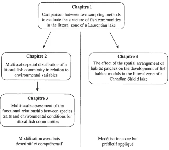
Cette thèse propose de modéliser la structure spatiale des communautés de poissons lacustres en relation avec les facteurs environnementaux littoraux. La réalisation de cet objectif fut effectuée en utilisant une approche multiscalaire, c’est-à-dire en modifiant certains attributs relatifs à l’échelle d’analyse spatiale. Ces changements ont permis la modélisation de la structure des communautés de poissons à deux niveaux, d’une part dans un contexte decriptif/compréhensif et d’autre part, dans une contexte prédictif/appliqué (Figure 1.3).
L’étude de l’impact de la structuration spatiale de la zone littorale des lacs sur les communautés de poissons nécessite une technique d’échantillonnage qui soit continue dans l’espace. Le Chapitre 1 suggère l’utilisation du recensement visuel comme technique d’échantillonnage des communautés de poissons lacustres. Cette technique permet d’effectuer un inventaire des espèces de poissons et des variables environnementales en minimisant les perturbations sur l’habitat (Hall et Werner 1977). L’application de cette méthode dans un environnement lacustre nécessite toutefois certains ajustements. Une analyse comparative des limites avec une
Introduction générale 9 méthode d’échantillonnage plus traditionnelle, la seine de rivage, est présentée dans ce premier chapitre.
Chapitre 1
Comparison between two sampling methods to evaluate the structure of fish communities
in the littoral zone of a Laurentian lake,)
/
\
Chapitre 2 Chapitre 4
Multiscale spatial distribution of a The effect of the spatial arrangement of littoral fish community in relation to habitat patches on the development of flsh
I
environmental variables habitat modets in the littoral zone of a______________________________
Canadian Shield lake
Chapitre 3
Multi-scale assessment of the functional relationship between species
traits and environmental conditions for littoral fish communities
Modélisation avec buts Modélisation avec but
descriptif et compréhensif prédictif appliqué
Figure 1.3 Schématisation de la structure de la présente thèse en quatre chapitres.
Les approches statistiques offrent un contexte théorique pertinent pour l’étude des
patrons de distribution spatiale des espèces littorales et pour l’étude des processus
écologiques potentiels générant les assemblages d’espèces dans la zone littorale des lacs. Au Chapitre 2, nous avons appliquée une approche mathématique récemment développée par Borcard et Legendre (2002) et Borcard et coIl. (2004) sur une communauté de poissons littoraux d’un lac du Bouclier Canadien (Lac Drouin). Quatre hypothèses furent testées: (1) la variance de la communauté de poissons
littoraux d’un lac peut se décomposer en des fractions de variance correspondant à différentes échelles spatiales; (2) la structure de la communauté des poissons perçue à différentes échelles peut être associée à différentes variables environnementales qui fluctuent selon ces échelles; (3) les échelles spatiales et les variables environnementales structurant la communauté de poissons varient sur une échelle temporelle; (4) les espèces se classifient comme généralistes ou spécialistes selon la gamme d’échelles spatiales auxquelles elles sont associées.
La diversité des espèces peuplant la zone littorale des différents lacs et la pluralité de réponses des espèces à l’hétérogénéité spatiale de la zone littorale, soulignent la complexité que peut représenter l’élaboration de modèles d’utilisation d’habitat de poissons littoraux dans les lacs. Alors que les lacs présentent des différences appréciables au niveau de leur composition spécifique, ils partagent généralement les mêmes groupes fonctionnels d’espèces (Dfaz et coll. 199$, Nygaard et Ejrnaes 2004). La classification des communautés de poissons en groupes fonctionnels d’espèces partageant des traits biologiques similaires, représente donc un outil facilitant l’élaboration de modèles d’habitat de poissons. Dans le troisième chapitre, nous avons vérifié si les traits comportementaux et morphologiques des espèces de poissons littoraux de deux lacs situés sur le Bouclier Canadien, déterminaient la distribution spatiale de ces espèces. Plus précisément, nous avons vérifié: (1) la présence de groupes fonctionnels résultant de la concordance entre les différents traits comportementaux et morphologiques des espèces, (2) si les espèces constituant un même groupe fonctionnel étaient influencées par les mêmes conditions
Introduction générale 11 environnementales et (3) si ces relations traits-environnement possédaient une structure spatiale hiérarchique.
Alors que les chapitres précédents mettaient l’emphase sur des aspects fondamentaux (c.a U. descriptifs et compréhensifs) de la structuration spatiale des communautés de poissons littorales, le Chapitre 4 proposait une application pratique de l’intégration de la structuration spatiale dans des modèles prédictifs d’habitat de poissons. Un nombre grandissant d’études reconnait l’influence non seulement des conditions environnementales locales, mais également de la taille et de l’arrangement spatial des différents habitats sur les communautés de poissons (Essington et Kitcheil 1999). Ainsi, le quatrième chapitre testait: (1) l’impact de la taille des unités d’analyse sur la performance des modèles d’habitats et (2) les contributions relativs des variables environnementales locales et des variables environnementales relatives à l’arrangement spatial des sites. Pour ce faire, trois approches furent comparées: (1) une approche dite de sites, dont l’unité d’analyse était équivalente à la dimension des sites d’échantillonnage, (2) une approche dite constante-multiple, dont l’unité d’analyse était constituée de groupements croissants de sites (c.-à-d. 1S, 2S, 3S, etc.) et (3) une approche dite de taches d’habitat, dont l’unité d’analyse correspondait à des groupements de sites contigus partageant les mêmes caractéristiques environnementales. En comparant ces diverses approches statistiques, le quatrième chapitre se voulait une contribution à une meilleure utilisation des modèles prédictifs d’habitat à l’échelle d’un lac.
Comparison between two sampling methods to evaluate the
structure offish communities in the littoral zone ofa
Laurentian lake
A. Brind’Arnour and D. Boisclair Journal of Fish Biology 65 :1372-1384
Chapitre 1 Recensement visuel 12
AB STRACF
The resuits of beach seining were compared with visual surveys, in habitats showing a gradient of macrophyte densities in Lake Drouin, Québec, Canada. Six comrnunity descriptors (species density, total fish density, relative abundance per species, presence or absence of given species, size structure of the fish community and total biomass of the fish community) were used to compare the sampling methods. Most of the fish commtinity descriptors obtained by visual surveys were estimated with an accuracy similar to that of beach seining. Both methods sampled the same number of species (eight out of nine). Visual surveys assessed the relative abundance of the yellow perch Perca Jtavescens and white sucker Catostomus commersoni with an higher accuracy than the beach seine. The greatest discrepancies between the two sampling methods were for total fish density and the total fish biomass. Because of the sampling strategy, both descriptors were underestimated by visual surveys, notably in the higher macrophyte density. In a broad community survey to determine the relative importance of species abundance, the visual survey was effective and could be used to develop a within-lake regular and fine-scale sampling design of the spatial arrangement of fish communities and their habitats.
INTRODUCTION
The purpose of fish habitat models is to describe and eventually to predict the effects of natural and anthropogenic perturbations on measures of fish performance (e.g. abundance, survival, reproduction, growth). Many studies developed relationships between measures of fish performance and environmental conditions (Werner et aI. 1977, Brazner and Magnuson 1994, Randall et al. 1996). The identification of the proper spatial scale (s) at which the existence of such relationships should be tested and the relative significance of processes occurring at these scales, however, remains the key problem of habitat models (Lewis et al. 1996, Mason and Brandt 1996). fundamental contributions to the development of spatially explicit (Brandt et al. 1992) and individual-based models (Kocik and Ferreri 199$, Essington and Kitchell 1999) illustrate the recognition that fish may flot only be affected by local environrnental conditions, or by the quantity of habitats possessing specific key characteristics, but also by the spatial arrangement of habitats (Essington and Kitcheil 1999). Proper analysis of the effect of the spatial arrangement of environmental conditions on fish requires a spatially continuous sampling design. The feasibility of conducting spatially continuous sampling surveys depends on fish community complexity, habitat structure. and methodological limitations.
The littoral zone of lakes is generally recognised as a productive, diverse, and physically heterogeneous environment (Wetzel 1990). As such, it bears a paiticularly interesting status for studies on biodiversity, conservation, and management. Beach seining is one of the most common methods used to sample the fish community of the littoral zone, because it allows the investigator to identify, count, and collect a suite of
Chapitre 1 : Recensement visuel 14 variables about the fish captured (Pierce et al. 1990). Furthermore, the volume or the surface area sampled by seining may be estimated with a precision that surpasses that of many other methods
(gui
nets, trap nets, etc). Because of logistical limitations, it is difficult to conceive that seining could be used to provide a spatialÏy continuous description of fish communities in the littoral zone of lakes. Visual sampling, like seining, us subjected to the potential problems offish avoidance and cryptic behaviour (Harmelin-Vivien et al. 1985). Benthic-oriented or smaÏl size species may hide within coarse substrate interstices or can escape beneath the lead une when seine approaches (Parsley et al., 1989). Visual sampling may allow the investigator to count and identify fish, and to estimate the area sampled. These are prerequisites for the developmentof a regular and fine-scale sampling design of the spatial arrangement of fish communities and of their habitats.No method can be expected to provide a complete and flawless quantitative description of the structure of the fish community in the littoral zone of lakes (Weaver et al. 1993). The comparison of different methods, however, may allow an increase in the understanding of the information provided by the analysis of data based on a specific sampling approach. The objective of the present study was to compare the descriptors (species density, total fish density, relative abundance per species, presence or absence of given species, size structure of the fish community and total biomass of the fish community) of the structure of the littoral zone fish community obtained by seining with values obtained by visual surveys. This comparison was performed to identify those variables obtained by visual surveys that may be estimated with an accuracy equal to, or higher than, that of seining and,
consequently, assessing the variables that may be the subject of spatially continuous sampling.
MATERIALs AND METHODS
Sttid take
Sampling was conducted in Lake Drouin (Lanaudière Region of Québec, Canada; 46°09’ N : 73°55’ W) during the spring and summer periods of 2001 (Figure 1.1). Lake Drouin was selected for this study because it has a diversified littoral zone with woody debris, rocky substrate, sand beaches, and patches of macrophytes of mixed species such as water shield Brassenia schreberi, pipewort Eriocauton aquaticum, Eurasian milfoil Myriophyltum spicatum, and waterlillies Nymphea sp. This mesotrophic lake has a surface area of 31 ha and a maximum depth of 22 m. The water column is thermally stratified from May to October. During this period, surface water temperature ranges from 15°C to 26°C and bottom temperature ranges from 4°C to 8°C. The thermocline forms at 4.5 m depth in mid-June and breaks down in ear!y October.
Sampling procedures
The structure of the littoral zone fish community was assessed at 10 sites in Lake Drouin. The number of sites surveyed corresponded to the maximum number of seine hauls (c. 40 min per seine haul including collecting fish data) that could be completed within a sampling interval of e. 6 h (from 900 hours to 1500 hours). This criterion was used in an attempt to minimise the effect of potential changes on fish community attributes over the die! cycle (dusk, mid-day, dawn, night; Keast and Harker 1977).
Chapitre Ï Recensement visuel 16 The 10 sites were selected on the basis of information collected during a pre
sampling survey (6 June 2001). During this pre-sampling phase, the littoral zone at any potential sampling site was described using average water depth, substrate
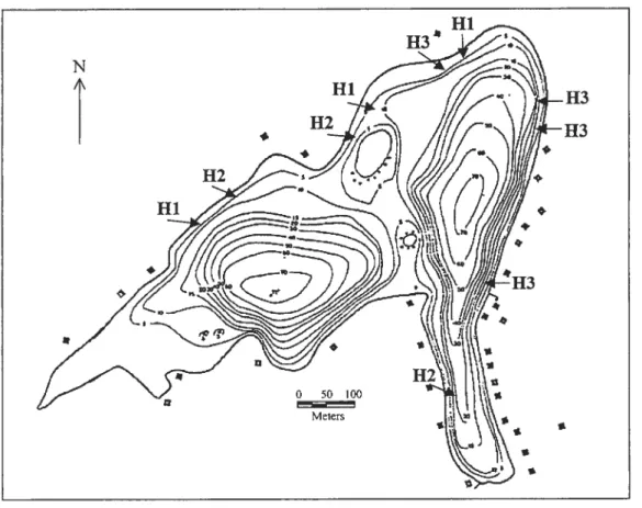
Figure 1 .1 Location of the ten sites classified by the three classes of habitat (H) at Lake Drouin (Quebec). Black squares along the lake contour represent houses and cottages.
composition, and potential for macrophyte development (Table 1.1). Average water depth in each sampling site was measured at three locations along a transect perpendicular to shore (25, 50 and 100% of the width of a sampling site). The average of the three measures was used in the statistical analysis. Sites with a silty substrate on which dead macrophytes could be seen were considered as potential sites for macrophyte growth.
T
Hi 112 Hi H3 H3 * 4 0 50 100 Meters sMacrophyte Average Sand Boulder Woody Habitat
density water depth debris category
(stem m2)2 (m) 0.50 2.34 1 0 0 2 12.25 0.84 0 1 0 3 0.00 1.35 1 0 0 1 42.75 0.89 0 1 0 3 0.75 3.01 1 0 0 1 1.00 2.19 1 0 0 2 0.00 2.52 0 1 0 1 13.75 2.58 0 0 1 2 14.75 2.52 1 0 0 3 7.75 1.81 0 0 1 2
Table 1.1 Description of the four environmental characteristics. Macrophyte density was estimated by the individual per m2 and the different types of substrate were expressed as binary variables. Site Macrophyte density (stem m2)1 Ï 3.50 2 7.25 3 0.00 4 32.75 5 0.25 6 1.80 7 0.50 8 2.25 9 32.25 10 1.50 =June,2=August.
The sampling sites used were selected using three criteria: the surface area of the sites, the within-site homogeneity, and the among-site diversity. The minimum surface area of the sampling sites (200 m2) was determined by the maximum surface area sampled by our seine and by our intention to associate site-specific series of fish community descriptors to well-defined habitat types. The length of a sampling site (35 to 70 m) was defined by its dimension along shore. The width of a sampling site (5 to 10 m) was determined by the distance from shore to the 3 m depth isobath. The limit of 3 m was adopted because it corresponded to the depth at which ail fishes observed could be identified and counted in the lake. Sampling sites had to possess relatively homogenous attributes in respect to a given combination of variables used
Chapitre 1 Recensement visuel 1$ to describe the sampling sites over at least 80% of their surface area (160 m2). Finally, the sampling sites selected had to cover the complete range of combinations of average water depth, substrate composition, and potential macrophyte density in the littoral zone of the lake.
The sampling phase consisted in the estimation of water transparency, macrophyte density, and fish community structure at the ten sampling sites selected during the pre-sampling phase. Water transparency at each sampling site was measured with a Secchi disk above the 4.5 m depth contour at c. 1400 hours every day that the visual surveys were done. Water transparency was aiways equal to 4.5 m (bottom). Thus water transparency probably did flot limit the capacity to perform visual surveys from shore to the 3 m depth. Among-site variations of water transparency were minimal and they had no effect on the comparisons of fish community data among sites.
Sampling for macrophyte and flsh were both performed from 19 to 26 June (further referred to as June) and from 28 July to 5 August 2001 (further referred to as August). This strategy was adopted to insure adequate temporal matching between data collected for macrophytes and fish. The density of macrophytes at the tel sites was estimated by two snorkellers on 25 June and 2 August 2001. Whenever fish sampling was conducted on the same day as macrophyte sampling, the fish sampling was always done prior to the sampling of macrophyte to avoid fish disturbance. The density of macrophytes at each site was estimated in four randomly selected 1 m2 quadrats (a 1 m2 frame was thrown from centre of the sampling site in different directions within each site). The number of stems from submersed, from ernergent,
and from leaf-floating forms per Ï m2 was counted and summed. The average number of stems from the four replicates was used in the statisticai analysis.
The sampiing of the fish community using the seine and the visual surveys was conducted between 19 and 26 June 2001 and between 28 July and 5 Augtist 2001. A number (from 1 to 10) was assigned to each sampling site and represented the temporal order in which they were sampled during one day. This order was maintained for the different sampling days and sampling methods (seine and visuai samplings).
Seining was performed on 19 and 23 June and on 2$ July and 5 August. Seining was done during the day between 1000 and 1600 hours with a 50 m x 3 m beach seine (mesh size = 1 cm). At each sampiing site, one seine haul of rectangular shape that covered a surface area of 260 m2 (s.D. = 51.639) was performed from a small boat propelied by an electric motor to minimise noise and fish disturbance. The seine was deployed such that it always extended to the 3 m depth isobath. The fishes captured were immediateiy identified, counted, and measured. The total Iength (LT, to the
nearest 0.25 cm) of a maximum of twenty fish per species was measured. The twenty fish per species were selected to cover the compiete size range sampied for this species. The ratios between the number of fish measured over the number of fish captured were over 75% for ail the species, except for Lepomis gibbosus (Linnaeus) for which 38% of the individuais captured were actuatiy measured. While seining, a snorkeller was prepared to free the seine from obstacles whenever necessary. This strategy was used to improve capture efficiency.
Chapitre 1 $ Recensement visuel 20
Visual surveys used to describe the fish community were conducted on 25 and 26 June and on 3 and 4 August during the day between 1000 and 1400 hours using a modified version of the technique described by Harmelin-Vivien et al. (1985). This technique requires two observers who snorkel at the water surface performing zigzags over the complete length and width of a sampling site following a trajectory that was globally parallel to shore. During such sampling, the distance between the two observers was e. 4 m. This technique allowed the observers to cover 90% of the total area of each sampling site. The observers maintained a constant swimming speed of c. 10 m min1 to minimise fish disturbance (Ekhiv 1997). Data were noted on polyvinyl chloride (PVC) cylinders that snorkellers wore around their forearm. Snorkellers identified the species, the relative abundance, and the approximate size of the fish observed as they progressed along their respective transect. The relative abundance of fish was defined in six classes: class 1 = 1 individual; class 2 2 individuals; class 3 = 3 individuals; class 4 = 4-5 individuals; class 5 = 6-9 individuals and class 6 = 10 individuals and more. Each fish was also categorised according to its size (Table 1.2). The classification of fish size was based on specific ecological information extracted from Scott and Crossman (1973). For instance, the distinction between small individuals (juveniles) and large individuals (adults) for Catostornus coinmersoni (Lacepede), was based on the minimum size (160 mm) at which the individuals shift from ptankton feeding to bottom feeding. This approach, applied to ail fish species present in Lake Drouin resulted in the definition of three size classes: SC1 = shorter than 110 mm Lr; SC2 = 110-160 mm L; SC3= longer than 160 mm L.
Coinputations
The flsh community was characterised using six descriptors: total number of species, total fish abundance, relative abundance per species, presence or absence of given species, size structure of the fish community, and total biomass of the fish community. Each of these descriptors was estimated for each sampling site using data collected by seining and by visual surveys. Since the surface area sampled varied among the sampling sites, the total number of species and the total fish abundance were calculated per unit area. This operation leU to the creation of two additional descriptors of the fish community: the species density and total fish density. These newty estimated descriptors were used in the statistical analyses instead of the original abundance descriptors. The relative abundance per species was calculated by converting species abundances from each site into a percentage. The size structure of the fish community at each sampling site was described by the percentage of fish (C1)
in the three size classes (SC1: SC2; SC3):
C1=(n1N’) 100 (1)
where n1is the number of fishes of a given size class i and N is the total abundance of
fish at a sampling site. Since the abundance data (tz1) obtained with the visual surveys
were collected in classes, we transformed them to abundance values as follow: 1
(
1individual), 2
(=
2 individuals), 3 (3 individuals), 4(=
5 individuals), 5(=
$individuals) and 6
(=
10 individuals). This change of state of the abundance data fromChapitre 1 : Recensement visuel 22 Table 1.2 Size range, measured with a precision equal to ± 2.5 mm. for each species sampled in the community. The asterisk identifies the species sampled with the seine and the visual surveys. Common names are in parenthesis.
Lrrange Method
Species Code (mm) Seine Visual
Pimephales prometasRafinesque (fathead Pipr 40-90 *
mi nnow)
Percaflavescens Mitchiil (yellow perch) Pefi 55-230 * * Lepomis gibbosus Linnaeus (pumpkinseed) Legi 30-195 * *
Ameriurus nebutosusLesueur (brown Amne 50-190 * *
bullhead)
Notemigonus crysoteucas Mitchili (golden Nocr 65-225 * * shiner)
Sernotilus atrornaculatus Mitchili (creek Seat 55-135 * chub)
Catostomus comniersoniLacepede (white Caco 55-320 * *
sucker)
Fundutusdiaphanus Lesueur (banded Fudi 50-85 * *
killifish)
Umbra tirni Kirtiand (central mudminnow) Urnli 50-100 *
The total biomass (BT) of fishes for any combination of species and size class was
estimated as:
= n PsI (2)
where n is the number of fish per species per size class and M1 is the average fish mass (grams) per species per size class estimated using the length-mass relationships in Schneider et al. (2000) and from relationships estimated in our laboratory for
Laurentian lakes (Comeau & Boisclair, unpublished). The total fish biomass was also divided by the surface area of each sampling site.
Statistical analyses
The 10 sites were partitioned among three groups of habitat defined by average water depth, composition of the substratum and density of macrophytes. A discriminant analysis using a stepwise method was used to estimate the linear combinations of the environmental variables (average water depth, substratum composition and macrophyte density) that were maximally effective in distinguishing the groups of habitats. Because the discriminant analysis suggested that only macrophyte density significantly contributed to the variation among sampling sites, the different habitat types (H) were defined according to macrophyte densities: Hi, low macrophyte density ranging from 0.00 to 1.80 stems m2; H2, medium macrophyte density ranging from 0.50 to 13.75 stems m2; H3, high macrophyte density ranging from 7.25 to 42.75 stems m2. The new habitat variable was subsequently used as a main factor in the statistical analysis comparing the two sampling methods. This discriminant analysis was carried out with SPSS (SPSS, 1999).
Statistical analyses on the multivariate fish community descriptors were done using a multivariate analysis of variance (MANOVA) design with covariates. Statistical analyses on the univariate fish community descriptors were done using an analysis of variance (ANOVA) design with covariates. The main factors in the MANOVA and the ANOVA were the sampling method (M), the type of habitat (H), and the sampling month (Mo). Because the fish sampling using the seine and the
Chapitre 1 : Recensement visuel 24 visual surveys were flot conducted on the same day, two dummy variables representrng the sampling days were used as covariates. These dummy variables were orthogonal with each other (i.e. their sum = 0). The first dummy variable coded for the seine sampling days: with 1 for the first day of the seine sampling, with —1 for the second day of seine sampling, and with O for the 2 days of visual surveys. The second dummy variable was coded with O for the 2 days of seine sampling and 1 and —1 for the 2 days of sampling with the visual surveys. The site numbers defining the temporal order in which the sampling was conducted were also used as covariates. A significant effect of the factor M or the interaction terms M x H, M x Mo or M x H x Mo was interpreted as a difference between the two sampling methods in describing the fish community. Since the main interest was the comparison between the sampling methods, only the resuits for those terms were discussed. Statistical analyses were carried out with SPSS (SPSS, 1999), using a significance threshold of 0.05. A posteriori multiple comparisons were done on the 95% confidence intervals of the interaction terms (M x H, M x Mo, M x H x Mo) using the Bonferroni correction for multiple testing (Sokal and Rohlf 1995). Partial correlation analyses, controlling for the site numbers, were conducted on fish community descriptors showing discrepancies between the two sampling methods. Normality was tested using the Shapiro-Wilks statistics (Zar 1984). Heterogeneity of variance was sometimes observed, but the analysis of variance is relatively robust to unequal variances provided that a fixed model is used (Bray and Maxwell 1985). The Hellinger transformation (Legendre and Gallaglier 2001) was computed on the