Influence of motion on contrast perception: supra-threshold spatio-velocity CSF measurements

(1)

HAL Id: hal-00252676

https://hal.archives-ouvertes.fr/hal-00252676

Submitted on 12 Feb 2008

HAL is a multi-disciplinary open access

archive for the deposit and dissemination of

sci-entific research documents, whether they are

pub-lished or not. The documents may come from

teaching and research institutions in France or

abroad, or from public or private research centers.

L’archive ouverte pluridisciplinaire HAL, est

destinée au dépôt et à la diffusion de documents

scientifiques de niveau recherche, publiés ou non,

émanant des établissements d’enseignement et de

recherche français ou étrangers, des laboratoires

publics ou privés.

Influence of motion on contrast perception:

supra-threshold spatio-velocity CSF measurements

Sylvain Tourancheau, Patrick Le Callet, Dominique Barba

To cite this version:

Sylvain Tourancheau, Patrick Le Callet, Dominique Barba. Influence of motion on contrast perception:

supra-threshold spatio-velocity CSF measurements. Human Vision and Electronic Imaging XII., Feb

2007, San Jose, CA, United States. pp.64921M. �hal-00252676�

(2)

Influence of motion on contrast perception: supra-threshold

spatio-velocity CSF measurements

Sylvain Tourancheau, Patrick Le Callet and Dominique Barba

Université de Nantes – IRCCyN laboratory – IVC team

Polytech’Nantes, rue Christian Pauc, 44306 Nantes, France

ABSTRACT

In this paper, a supra-threshold spatio-velocity CSF experiment is described. It consists in a contrast matching task with a methods of limits procedure. Results enable the determination of contrast perception functions which give, for given spatial and temporal frequencies, the perceived contrast of a moving stimulus.

These contrast perception functions are then used to construct supra-threshold spatio-velocity CSF. As for supra-threshold CSF in spatial domain, it can be observed that CSF shape changes from band-pass behaviour at threshold to low-pass behaviour at supra-threshold, along spatial frequencies. However, supra-threshold CSFs have a band-pass behaviour along temporal frequency has threshold one. This means that if spatial variations can be neglected above the visibility threshold, temporal ones are still of primary importance.

Keywords: supra-threshold CSF, spatio-velocity CSF, motion sensitivity, contrast perception

1. INTRODUCTION: MOTIVATIONS AND BACKGROUND

The way the human visual system (HVS) perceives contrast is of central importance in the understanding of most visual tasks. The contrast sensitivity function (CSF) describes the sensitivity of the HVS to gratings (generally sinusoidal gratings) as a function of spatial frequency. Sensitivity is defined as the reciprocal of contrast threshold. Shape of CSF and its variations with changes in viewing conditions allow to make strong inferences about the underlying physiological processes.

A fine model of human visual system is required in different applications such as image or video psychovisual coding, development of quality assessment model, etc. In any HVS model, CSF is probably the most important stage. Successive stages generally depend on the good implementation of it. Typically, the CSF is measured by threshold detection measurements or supra-threshold contrast measurements. Both permit to quantitatively evaluate variations of HVS’s sensitivity over spatial frequencies.

Since natural images are composed of small details and shaped regions, its necessary to describe the contrast sensitivity of human visual system over spatial frequencies. Such a description is typically given by the contrast sensitivity function. Typically, it can be observed that the HVS is most sensitive to mid-frequencies around 4 cycles per degree (cpd). The sensitivity drops rapidly in higher frequencies and decreases slightly in lower ones. To measure the sensitivity of HVS over spatial frequencies, a stimulus with a given spatial frequency is presented to the observer and its contrast is modified until it becomes unseen. The same operation is repeated for different spatial frequencies, contrast thresholds are finally obtained for all the range of spatial frequencies. Sensibility is usually defined as the inverse of threshold contrast. Contrast sensitivity function can then be determined.

However, CSF is also influenced by temporal effects. Threshold detection measurements can be made over temporal frequencies for a fixed spatial frequency. Classic spatio-temporal CSF are measured with flickering stimuli, but different ways of adjusting temporal frequencies exist. When speaking about video, it is more natural to consider motion rather than flicker. Contrast sensitivity functions are then measured with moving stimuli

Further author information:

sylvain.tourancheau@univ-nantes.fr, +33 (0) 240 683 065 patrick.lecallet@univ-nantes.fr, +33 (0) 240 683 047

(3)

0 50 100 150 200 250 0.01 0.1 1 10 100 Temporal frequency (Hz) 0.1 1 10 Spatial frequency (cpd) 0 50 100 150 200 250 Sensitivity

Figure 1.Example of Kelly’s spatio-temporal CSF.

whose temporal frequency is determined by adjusting its velocity as a function of its fixed spatial frequency.

Such measurements are called spatio-velocity CSF. Kelly1_{has produced exhaustive measurements, which permit}

to show that HVS is more sensitive to moving stimuli rather than flickering ones with an approximate factor of 2. Kelly’s spatio-temporal CSF model is shown in Figure 1.

A Gabor pattern, such as those represented in figure 2, is often used in CSF measurements. It consists in a sinusoidal grating which is windowed by a radially symmetric Gaussian function that fades the pattern from its full contrast to the mean luminance. Three ways of moving this patch can be considered: 1. sine wave and window are in motion through the screen and eyes are tracking the pattern movement, 2. sine wave and window are in motion through the screen and eyes remain fixed at the center of the screen, 3. sine wave is in motion but window remain stationary on the center of screen and eyes keep fixed. Spatio-velocity CSF measurements have

been conducted2 _{for these three cases. It comes that case 1 gives statistically similar results as a classical CSF}

without any temporal variations. Furthermore, cases 2 and 3 lead to the same contrast sensitivity functions. No work has been found concerning supra-threshold temporal CSF, so it has been decided to conduct spatio-velocity supra-threshold CSF measurements. Indeed, it could be interesting to know the way that temporal variations induced by motion can affect perception of contrast strength.

If threshold detection CSF gives some interesting results concerning the ability of HVS to detect low con-trasted pattern, contrast perception measurements in supra-threshold lead to more useful results in the perspec-tive of modeling HVS response for natural scenes. In natural content, considered contrasts are generally well above threshold and to adapt threshold results to supra-threshold is not a simple task. Spatial supra-threshold CSF measurements found in literature works can be parted in three: contrast-magnitude estimation, contrast matching, contrast discrimination.

In contrast-magnitude estimation experiments,3, 4 _{subjects are asked to estimate contrast strength of one}

stimulus at a time by giving a rating number on an arbitrary open scale. In contrast matching experiments,4–6_two

stimuli are presented simultaneously and observers have to make them match in terms of contrast. Adjustment

can be done by the observer (for example, in an analogical way5_{or with a fixed variation step}6_{) or using a staircase}

(4)

Stimulus Spat. freq. Velocity Contrast

A Fs 0 Cs

B Fs V Cm

Table 1.Stimuli variable parameters.

has shown4 _{that contrast matching and contrast estimation measurements lead statistically to similar results.}

Contrast matching experiments show that perceived contrast plotted as a function of spatial frequency tends to vary from threshold CSF at low reference contrasts to constant value for high reference contrasts. This contrast constancy is also revealed by contrast estimation experiments.

In contrast discrimination experiments,7_{a staircase procedure with a forced-choice paradigm is used. Subjects}

are required to distinguish between two stimuli that are identical except for their contrast C and C + ∆C (C is the pedestal contrast and ∆C the contrast-increment). Differently from contrast matching measurements which are led in order to determine equally-perceived contrasts, purpose of contrast discrimination measurements is to determine the contrast-increment threshold, that is to say the value of ∆C for which the two stimuli are correctly discriminated. The relation between ∆C and C is called contrast-discrimination function. Contrast discrimination measurements generally lead to a dipper shaped function. ∆C first drops for pedestal contrast near the contrast detection threshold (for this facilitation effect, an analogy can be made with masking effects). Then, the contrast-increment rises steadily, following a power law (experimental value of exponent is generally found near 0.6) for supra-threshold pedestal contrasts. Furthermore, this relation between supra-threshold and threshold sensitivity doesn’t vary significantly with eccentricity.

2. MEASUREMENTS

In order to determine supra-threshold sensitivity to moving stimuli, it has been decided to design a contrast matching experiment using a method of limits procedure. In this part, experiment is described, procedure and experimental setup are precised.

In the following, contrast of a stimulus is defined as Michelson contrast given by this relation:

C= Lmax− Lmin

Lmax+ Lmin

, (1)

where Lmax(resp. Lmin) is the maximum (resp. minimum) luminance of the stimulus.

In the case of a sine pattern with an amplitude A and a mean luminance Lmean, this contrast can be expressed

as follows:

C= A

Lmean

. (2)

2.1. Experiment

Designed experiment is presented in Figure 2. The screen is vertically split into two equal parts in which two stimuli are simultaneously presented to the observer: a still sine pattern in the top part (stimulus A) and a moving one in the bottom part (stimulus B). Each of these two stimuli is spatially faded by a stationary Gaussian window. The width of the Gaussian window at half-height is set to two degrees.

The three variable parameters of each stimulus are named in Table 1. In each presentation, four of these

parameters are fixed: spatial frequency of the two stimuli Fs, velocity of the moving stimulus V and contrast of

the moving stimulus Cm. The task of the observer consists in the adjustment of the contrast of the still stimulus

Csuntil it perceptually matches the contrast of the moving stimulus Cm. These contrast matching measurements

have been done for four different contrasts Cm: 0.08, 0.15, 0.3 and 0.5.

Four spatial frequencies Fsof the two stimuli, and three temporal frequencies Ftof the moving stimulus have

been explored during these measurements. It results 12 points of the spatio-temporal domain as enumerated in Table 2. The values in cells are the corresponding velocities of the moving stimulus for these 15 conditions.

(5)

Figure 2.Design of contrast matching experiment. Spatial frequency (cpd) 1.6 3.2 6.4 12.8 Temporal 4.8 3 1.5 0.75 -frequency 9.6 6 3 1.5 0.75 (Hz) 19.2 12 6 3 1.5

Table 2.Moving stimulus velocity (in deg/s) for the 12 combinations of parameters.

The relation between the temporal frequency Ft, the spatial frequency Fsand the velocity V of the moving

stimulus is the following:

Ft= FsV. (3)

As its the contrast sensitivity relative to retinal velocity which has to be determined, observers are asked to not track the moving stimulus. The stationary Gaussian window, associated with relatively high temporal frequencies, enables to easily respect this condition. However, a moving stimulus with a spatial frequency of 12.8 cpd and a temporal one of 4.8 Hz has a too slow retinal velocity (0.375 deg/s) to achieve this. This stimulus has thus been removed from the set.

2.2. Equipments and observers

Experiments have been made in a normalized room, with controlled brightness and chromaticity conditions. Stimuli are presented on a Samsung SyncMaster 1100MB CRT monitor at a refresh rate of 120Hz and with a

mean luminance of 50 cd/m2_{. At the viewing distance of 135 cm, the screen subtended 18}◦ _{horizontally and}

13.5◦ _vertically.

The displaying of the stimuli and the sequencing of the procedure have been performed with Matlab, using

the Psychophysics Toolbox extensions.8

Five observers with a perfectly corrected sight have participated to the experiment. They was familiar with the procedure, particularly with the fact they don’t have to track the moving stimulus. Each of them has repeated each of the 44 measurements three times, on different days and hours.

A session consists in three presentations. This assures a session length of 15 minutes maximum.

2.3. Procedure

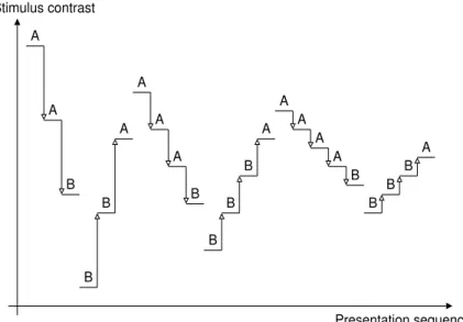
Chosen procedure is the method of limits as illustrated in Figure 3. The two stimuli are presented to the observer during five seconds. Then the letters A and B appears on the screen and the observer is asked to indicate the

(6)

Figure 3. Contrast determination using the method of limits. A and B assigned the stimulus which has been selected by the observer.

stimulus which seems to have the stronger contrast according to his perception. If the observer choose stimulus

A (still stimulus), the contrast Csis decreased. On the contrary, if he choose stimulus B (moving stimulus, the

contrast Csis increased.

This methodology permits to rapidly cover a large part of the contrast range by adjusting the variation steps. A measurement is considered completed when the observer has performed six paths, that is to say three back-and-forth. For each back-and-forth, the step of contrast variation is decreased, from 10% of the contrast range in the first path to the minimum value that display settings enable in the last one. For the two first paths (first back-and-forth), the starting values are maximum and minimum of the contrast range, respectively. In the two following back-and-forth, starting values are adjusted as function of final values of previous path. Finally, recorded contrast value is computed as the average of the final values of the four last paths.

3. RESULTS

3.1. Contrast perception functions

3.1.1. Measured data

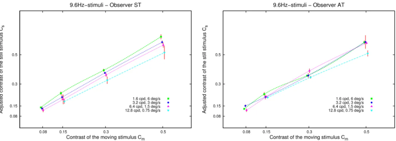
Figure 4 shows the contrast matching measurements of observers ST and AT with 9.6Hz-stimuli. Each point

puts in relation the contrast of the moving stimulus Cm(fixed) and the contrast of the still stimulus Cs(adjusted

by the observer until it perceptually matches Cm). For these two observers, it must be noticed that the

intra-observer confidence intervals are quite small, except for several points. This observation is verified for other observers.

For observer ST, the moving stimulus is perceived slightly weaker as its spatial frequency increases. For observer AT, contrast perception is roughly the same for stimuli of 1.6 cpd (6 deg/s), 3.2 cpd (3 deg/s) and 6.4 cpd (1.5 deg/s). Stimulus with highest spatial frequency (namely 12.8 cpd) and lowest retinal velocity (namely 0.75 deg/s) is perceived quite weaker, as for observer ST.

The mean results over the five observers have approximately the same behaviour as those of observer AT, as shown in Figure 5. The perception of the three fastest moving stimuli with the lowest spatial frequencies is roughly the same with regard to the size of confidence intervals. The slowest stimulus, with the spatial frequency of 12.8 cpd, is perceived weaker.

Results for 4.8Hz-stimuli and 19.2Hz-stimuli are presented in Figure 6. Here again, there is no significant differences in perception between the three fastest stimuli (i.e. with the three lowest spatial frequencies) with

(7)

0.5 0.3 0.15 0.08 0.5 0.3 0.15 0.08

Adjusted contrast of the still stimulus C

s

Contrast of the moving stimulus C_m 9.6Hz−stimuli − Observer ST 1.6 cpd, 6 deg/s 3.2 cpd, 3 deg/s 6.4 cpd, 1.5 deg/s 12.8 cpd, 0.75 deg/s 0.5 0.3 0.15 0.08 0.5 0.3 0.15 0.08

s

Contrast of the moving stimulus C_m 9.6Hz−stimuli − Observer AT

1.6 cpd, 6 deg/s 3.2 cpd, 3 deg/s 6.4 cpd, 1.5 deg/s 12.8 cpd, 0.75 deg/s

Figure 4.Contrast matching results for the four 9.6Hz-stimuli. Observers ST and AT. The horizontal shift of each data point is for clarity.

0.5 0.3 0.15 0.08 0.5 0.3 0.15 0.08

s

Contrast of the moving stimulus C_m 9.6Hz−stimuli − Mean observer

1.6 cpd, 6 deg/s 3.2 cpd, 3 deg/s 6.4 cpd, 1.5 deg/s 12.8 cpd, 0.75 deg/s

Figure 5.Contrast matching results for the four 9.6Hz-stimuli. Mean results over the five observers. The horizontal shift of each data point is for clarity.

regard to the size of confidence intervals. Moreover, the slowest 19.2Hz-stimulus (i.e. with the spatial frequency of 12.8 cpd) is perceived weaker than the others 19.2Hz-stimuli.

It can be noticed than the inter-observers confidence intervals are a bit larger than the intra-observer ones, as expected. Furthermore, these confidence intervals are larger, except for particular stimuli, as the contrast of

the moving stimulus Cm increases. This is due to the inter-observers differences, which are more important as

the visual perception task is moving away from a detection task.

For mid-range frequencies (1.6 cpd to 6.4 cpd in our experiments), the perception of a moving stimulus seems to not depend neither on its retinal velocity nor on its spatial frequency, but only on its temporal frequency (certainly the three parameters are linked). However, a decrease in perception is observed for the highest spatial frequencies, (resp. for the lowest retinal velocities).

Moreover, a variability along temporal axis can be observed. The contrast perception is maximum for 9.6Hz-stimuli, it decreases slightly for 4.8Hz-stimuli and more significantly for 19.2Hz-stimuli.

(8)

0.5 0.3 0.15 0.08 0.5 0.3 0.15 0.08

s

1.6 cpd, 3 deg/s 3.2 cpd, 1.5 deg/s 6.4 cpd, 0.75 deg/s 0.5 0.3 0.15 0.08 0.5 0.3 0.15 0.08

s

1.6 cpd, 12 deg/s 3.2 cpd, 6 deg/s 6.4 cpd, 3 deg/s 12.8 cpd, 1.5 deg/s

Figure 6. Contrast matching results for the three 4.8Hz-stimuli (left) and for the four 19.2Hz-stimuli (right). Mean results of the five observers. The horizontal shift of each data point is for clarity.

3.1.2. Model

The previous results give the adjusted contrast of the still stimulus Cs as a function of the contrast of moving

stimulus Cm for given spatial and temporal frequencies. This can expressed as follows:

Cs= f(Fs,Ft)(Cm). (4)

For each spatial and temporal frequencies Fs and Ft, the contrast perception function f(Fs,Ft) can be

con-structed from the measured points by data fitting. To do this, a power law model has been chosen:

f(Fs,Ft)(x) = a + bx

c

, (5)

with parameters a, b and c adjusted for each couple (Fs,Ft) and c < 1.

It must be noticed that in Figures 4, 5 and 6, the measured points are connected with smooth curves in order

to enhance the readability of the plots. These curves aren’t the plotting of functions f(Fs,Ft).

3.2. Supra-threshold spatio-velocity CSF

Spatio-velocity CSF measurements in detection generally consists in the determination of the contrast for which

a moving stimulus becomes unseen to the observer.1 _{The visual sensitivity of the observer can then be computed}

from this threshold contrast. These experiments are similar to supra-threshold measurements in the case where

the contrast of the still stimulus Cs is zero, and where the contrast of the moving one Cmis adjusted to match

with it.

In order to build CSF with our measurements, it’s necessary to know the contrast of the moving stimulus Cm

which perceptually matches a given contrast Csfor different spatio-temporal frequencies (Fs, Ft). This relation

is the inverse of relation 4, that is to say:

Cm= f_(F−1_s_,F_t₎(Cs). (6)

Some supra-threshold spatio-velocity 2D-CSF are then obtained.

Figure 7 shows the results of this contrast matching (Cs ≡ Cm) for a given temporal frequency Ft, along

(9)

1 0.5 0.1 0.05 30 10 5 1 0.5 1 5

Contrast of the moving stimulus C

m

Spatial frequency (cpd)

Contrast matching for F_t = 4.8 Hz

Velocity (deg/s) Cs = 0.15 Cs = 0.20 Cs = 0.30 Cs = 0.50 1 0.5 0.1 0.05 30 10 5 1 0.5 1 5 10

m

Velocity (deg/s) Cs = 0.15 Cs = 0.20 Cs = 0.30 Cs = 0.50 1 0.5 0.1 0.05 30 10 5 1 1 5 10

m

Velocity (deg/s)

Cs = 0.15

Cs = 0.20

Cs = 0.30

Cs = 0.50

Figure 7.Results of contrast matching at the three explored temporal frequencies and for four different reference contrast Csas a function of spatial frequency and retinal velocity (both are linked by relation 3). Both axis are in log scale, Y-axis

is inverted. Computed data are fitted with a Gaussian function in order to ease readability.

figures, both axis are in log scale and Y-axis is inverted. Then computed data are fitted with a Gaussian function in order to ease readability.

It can be observed there are no significant variations in shape between the three temporal frequency in Figure 7: curves have the same low-pass shape along spatial axis. These results agree with those obtained for

purely spatial supra-threshold CSF.3 _{Moreover, sensitivity is the same along spatial axis, except for high spatial}

frequencies where it falls. The cutoff frequency is roughly the same for a given temporal frequency: there is no

variations with the reference contrast Cs.

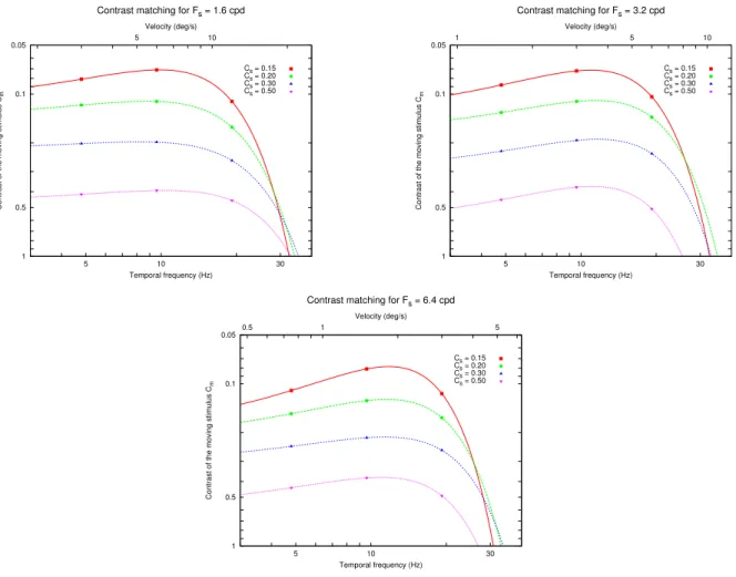
In Figure 8, curves along temporal axis have a band-pass shape. For the three fixed spatial frequencies, the peak of sensitivity occurs approximately for the same temporal frequency. It’s interesting to notice that the position of this peak is constant with respect of temporal frequency but not with respect of retinal velocity.

Same observations have been made at threshold.1

In order to speak in terms of sensitivity, a relative sensitivity can be defined as the ratio between the reference

still contrast Csand the adjusted moving one Cm:

Sr=

Cs

Cm

(10)

1 0.5 0.1 0.05 30 10 5 10 5

m

Temporal frequency (Hz)

Contrast matching for F_s = 1.6 cpd

Velocity (deg/s) Cs = 0.15 Cs = 0.20 Cs = 0.30 Cs = 0.50 1 0.5 0.1 0.05 30 10 5 10 5 1

m

Velocity (deg/s) Cs = 0.15 Cs = 0.20 Cs = 0.30 Cs = 0.50 1 0.5 0.1 0.05 30 10 5 5 1 0.5

m

Velocity (deg/s)

Cs = 0.15

Cs = 0.20

Cs = 0.30

Cs = 0.50

Figure 8.Results of contrast matching at the three explored spatial frequencies and for four different reference contrast Cs as a function of temporal frequency and retinal velocity (both are linked by relation 3). Both axis are in log scale,

Y-axis is inverted. Computed data are fitted with a Gaussian function in order to ease readability.

This relative sensitivity is shown in Figure 9 for the same results as those in Figure 8. This representation allows to appreciate the differences as the reference contrast increases. It’s observed that, in opposition to along spatial axis, the supra-threshold CSFs along temporal axis still have a band-pass behaviour as the reference contrast increases. As a consequence, if spatial variations can be neglected above the visibility threshold, it’s not the case for temporal variations which still influence the visual perception.

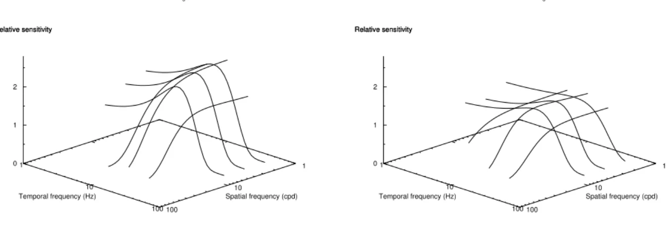
The relative sensitivity functions (along temporal axis as in Figure 9 and along spatial axis constructed from

Figure 7) have been plotted in the spatio-temporal domain for reference contrasts Cs = 0.15 and Cs = 0.50

(Figure 10). For low reference contrast (Cs= 0.15), the spatio-temporal CSF has a band-pass behaviour along

temporal axis, and the band-pass behaviour along spatial axis at threshold have changed to low-pass one above threshold.

When increasing the reference contrast (Cs = 0.50), the behaviour along temporal axis changes from

band-pass to low-band-pass shape. Well above threshold, the spatio-temporal CSF have a global low-band-pass shape, when near threshold a band-pass behaviour is still present along temporal axis.

The relative sensitivity depicts how strong a stimulus is perceived with respect to his spatio-temporal

char-acteristics. If Sr>1, the adjusted contrast Cm which perceptually matches the reference contrast Cs is weaker

than Cs, in other terms the moving stimulus is perceived stronger than it actually is. Here, in the case of a

(11)

0.5 1 1.5 2 2.5 30 10 5 10 5 Relative sensitivity C s /C m Temporal frequency (Hz)

Relative sensitivity for Fs = 1.6 cpd Velocity (deg/s) Cs = 0.15 Cs = 0.20 Cs = 0.30 Cs = 0.50 0.5 1 1.5 2 2.5 30 10 5 10 5 1 Relative sensitivity C s /C m Temporal frequency (Hz)

Relative sensitivity for Fs = 3.2 cpd Velocity (deg/s) Cs = 0.15 Cs = 0.20 Cs = 0.30 Cs = 0.50 0.5 1 1.5 2 2.5 30 10 5 5 1 0.5 Relative sensitivity C s /C m Temporal frequency (Hz)

Relative sensitivity for F_s = 6.4 cpd

Velocity (deg/s)

Cs = 0.15

Cs = 0.20

Cs = 0.30

Cs = 0.50

Figure 9. Relative sensitivity at the three explored spatial frequencies and for four different reference contrast Cs as a

function of temporal frequency and velocity (both are linked by relation 3). X-axis is in log scale. Computed data are fitted with a Gaussian function in order to ease readability.

1 10 100 1 10 100 0 1 2 Relative sensitivity Reference contrast Cs=0.15 Spatial frequency (cpd) Temporal frequency (Hz) Relative sensitivity 1 10 100 1 10 100 0 1 2 Relative sensitivity Reference contrast Cs=0.50 Spatial frequency (cpd) Temporal frequency (Hz) Relative sensitivity

Figure 10.Spatio-velocity supra-threshold CSF surface in the spatio-temporal domain, for two reference contrast: Cs=

(12)

increases and conversely. The surface of the spatio-temporal domain for which retinal motion induces an increase of perception is reducing as the reference contrast is growing away from threshold.

4. CONCLUSION

Subjective measurements have been led in order to understand the influence of motion on the contrast perception. The experiment consists in the contrast matching of two stimuli. First one is immobile with a varying contrast

Cs. Second one, with the same spatial frequency, is moving with a given speed and its contrast Cm is fixed.

Observers are asked to adjust the contrast Cs until it perceptually matches the contrast of the moving stimulus

Cm. Results of these measurements lead to contrast perception functions. These functions are quite similar over

mid-range spatial frequencies.

Then, these contrast perception functions are used in order to construct spatio-velocity supra-threshold contrast sensitivity functions. It’s observed that in spatial dimension these spatio-velocity supra-threshold CSFs

have the same behaviour as purely spatial supra-threshold CSF.3 _{That is to say: their shape changes from}

low-pass near threshold into band-pass for higher reference contrasts. In temporal domain, results are different. The band-pass behaviour at threshold is still present well above threshold. Furthermore, sensitivity variations

depend on temporal frequency rather than on retinal velocity, as in threshold experiments.1

These results confirm that above the visibility threshold, the spatial variations haven’t as much influence as at threshold. On the opposite, temporal variations, and particularly those induced by motion, lead to important differences in supra-threshold sensitivity.

REFERENCES

1. D. H. Kelly, “Motion and vision. II. Stabilized spatio-temporal threshold surface,” Journal of the Optical Society of America A 69, pp. 1340–1349, October 1979.

2. J. Laird, M. Rosen, J. Pelz, E. Montag, and S. Daly, “Spatio-velocity CSF as a function of retinal velocity using unstabilized stimuli,” in Proc. SPIE Conf. Human Vision and Electronic Imaging XI, 6057, Electronic Imaging 2006, Janvier 2006.

3. M. W. J. Cannon, “Perceived contrast in the fovea and periphery,” Journal of the Optical Society of America A 2, pp. 1760–1768, October 1985.

4. E. Peli, J. Yang, R. Goldstein, and A. Reeves, “Effect of luminance on suprathreshold contrast perception,” Journal of the Optical Society of America A 8, pp. 1352–1359, August 1991.

5. M. A. Georgeson and G. D. Sullivan, “Contrast constancy: deblurring in human vision by spatial frequency channels,” The Journal of Physiology 252, pp. 627–656, November 1975.

6. E. Peli, L. Arend, and A. T. Labianca, “Contrast perception across changes in luminance and spatial fre-quency,” Journal of the Optical Society of America A 13, pp. 1953–1959, October 1996.

7. G. E. Legge and D. Kersten, “Contrast discrimination in peripheral vision,” Journal of the Optical Society of America A 4, pp. 1594–1598, August 1987.