Brownian dynamics simulations of fine-scale molecular models

Brownian Dynamics Simulations of Fine-Scale Molecular

Models

by

Irina Burmenko

B.S. Chemical Engineering

Purdue University (2000)

Submitted to the Department of Chemical Engineering

in partial fulfillment of the requirements for the degree of

Master of Science in Chemical Engineering

at the

SSACHUSETT SIN TU OF TECHNOLOGY

JUN 01 2005

LIBRARIES _

MASSACHUSETTS INSTITUTE OF TECHNOLOGY

June 2005

( Massachusetts Institute of Technology 2005

Signature

of Author...-- ... ..

... .

... ...

Department of Chemical Engineering

24 May 2005

Certified

by... ...-..

..

IIIIIIIII...

Robert C. Armstrong

Chevron Professor of Chemical Engineering

Thesis Supervisor

Accepted

by

...

... ... ...

.... ....

Daniel Blankschtein

Chairman, Committee for Graduate Students

MA

Brownian Dynamics Simulations of Fine-Scale Molecular Models

by

Irina Burmenko

Submitted to the Department of Chemical Engineering

on 24 May 2005, in partial fulfillment of the

requirements for the degree of Master of Science in Chemical Engineering

Abstract

One of the biggest challenges in non-Newtonian fluid mechanics is calculating the polymer con-tribution to the stress tensor, which is needed to calculate velocity and pressure fields as well as other quantities of interest. In the case of a Newtonian fluid, the stress tensor is linearly proportional to the velocity gradient and is given by the Newton's law of viscosity, but no such unique constitutive equation exists for non-Newtonian fluids. In order to predict

accu-rately a polymer's rheological properties, it is important to have a good understanding of the

molecular configurations in various flow situations. To obtain this information about molec-ular configurations and orientations, a micromechanical representation of a polymer molecule must be proposed. A micromechanical model may be fine scale, such as the Kramers chain

model, which accurately predicts a real polymer's heological properties, but at the same time

possesses too many degrees of freedom to be used in complex flow simulations, or it may be a coarse-grained model, such as the Hookean or the FENE dumbbell models, which can be used in complex flow analysis, but have too few degrees of freedom to adequately describe the rheology. The Adaptive Length Scale (ALS) model proposed by Ghosh et al. is only marginally

more complicated than the FENE dumbbell model, yet it is able to capture the rapid stress

growth in the start-up of uniaxial elongational flow, which is not predicted correctly by the simple dumbbell models.

The ALS model is optimized in order to have its simulation time as close as possible to that of the FENE dumbbell. Subsequently, the ALS model is simulated in the start-up of the uniaxial elongational and shear flows as well as in steady extensional and shear flows, and the results are compared to those obtained with other competing rheological models such as the Kramers

chain, FENE chain, and FENE dumbbell. While a 5-spring FENE chain predicts results that

are in very good agreement with the Kramers chain, the required simulation time clearly makes it impossible to use this model in complex flow simulations. The ALS model agrees better with the Kramers chain than does the FENE dumbbell in the start-up of shear and elongational flows. However, the ALS model takes too long to achieve steady state, which is something that needs to be explored further before the model is used in complex flow calculations. Understanding of this phenomena may explain why the stress-birefringence hysteresis loop predicted by the ALS model is unexpectedly small. In general, if polymer stress is to be calculated using Brownian dynamics

simulations, a large number of stochastic trajectories must be simulated in order to predict

accurately the macroscopic quantities of interest, which makes the problem computationally

expensive. However, recent technological advances as well as a new simulation algorithm called

Brownian configuration fields make such problems much more tractable. The operation count in order to assess the feasibility of using the ALS model in complex flow situations yields very

promising results if parallel computing is used to calculate polymer contribution to stress.

In an attempt to capture polydispersity of real polymer solutions, the use of multi-mode

models is explored. The model is fit to the linear viscoelastic spectrum to obtain relaxation

times and individual modes' contributions to polymer viscosity. Then, data-fitting to the

di-mensionless extensional viscosity in the startup of the uniaxial elongational flow is performed

for the ALS and the FENE dumbbell models to obtain the molecule's contour length, bmax.

It is found that the results from the single-mode and the four-mode ALS models agree much

better with the experimental data than do the corresponding single-mode and four-mode FENE

dumbbell models. However, all four models resulted in a poor fit to the steady shear data, which may be explained by the fact that the zero-shear-rate viscosity obtained via a fit to the dynamic data by Rothstein and McKinley and used in present simulations, tends to be somewhat lower than the steady-state shear viscosity at very low shear rates, which may have caused a mismatch between the value of 0 used in the simulation and the true r0 of the polymer solution.

As a motivation for using the ALS model in complex flow calculations, the results by Phillips, who simulated the closed-form version of the model in the benchmark 4:1:4

contraction-expansion problem are presented and compared to the experimental results by Rothstein and

McKinley [49]. While the experimental observations show that there exists a large extra pres-sure drop, which increases monotonically with increasing De above the value observed for a Newtonian fluid subjected to the same flow conditions, the simulation results with a

closed-form version of the FENE dumbbell model, called FENE-CR, exhibit the opposite trend. The

ALS-C model, on the other hand, is able to predict the trend correctly. The use of the ALS-C model in another benchmark problem, namely the flow around an array of cylinders confined between two parallel plates, also shows very promising results, which are in much better

agree-ment with experiagree-mental data by Liu as compared to the Oldroyd-B model. The simulation

results for the ALS-C and the Oldroyd-B models are due to Joo, et al. [28] and Smith et al.

[50], respectively.

Overall, it is concluded that the ALS model is superior to the commonly used FENE dumb-bell model, although more work is needed to understand why it takes significantly longer than the FENE dumbbell to achieve steady state in uniaxial elongational flows, and why the stress-birefringence hysteresis loop predicted by the ALS model is much smaller than that of the other rheological models.

Thesis Supervisor: Robert C. Armstrong

Acknowledgements

1

There are many people whom I would like to thank for making my stay at MIT enjoyable. First of all, I would like to thank my advisor, Bob Armstrong, for guiding me through my research and for helping me overcome the usual hurdles of graduate research. It meant a great deal to me that he understood and accepted my decision not to continue pursuing my Ph.D. I was also lucky to have Pat Doyle and Gareth McKinley as my committee members. Pat always found time to meet with me if I needed his help or advice, and I really appreciate his providing me with the Kramers chain code, which made writing this thesis that much easier and less stressful. A special thank you goes to Bob Armstrong's assistant, Melanie Miller, who has been helpful beyond words.

I would also like to thank past and present fluid mechanics group members. I will always be grateful to Jason Suen for spending countless hours with me explaining the principles of kinetic theory and guiding me in my research for the next two years. Even though I only met Indranil Ghosh once, his new rheological model served as basis for my research. My thanks also go to Yong Joo, Scott Phillips, Pankaj Doshi, Arvind Gopinath, Micah Green, and Theis Clarke for the many useful conversations that we had. I wish you guys all the best in your current and future endeavors.

My stay at MIT would not be nearly as memorable had it not been for some wonderful

friends that I made among my classmates: Saeeda, Greg, Nina, and Noreen. I am really glad that I got to know them, and I truly hope that our friendships will continue after we all leave MIT. It is the friendships outside of MIT that kept me happy and sane even when I had hit dead-ends in my research and nothing seemed to work. My friends Grisha, Inna, Olya, Marina,

1This work was supported by the ERC program of the National Science Foundation under Award Number EEC-9731680.

Bella, and Jay were always there for me a short drive or a phone call away with a kind word of support, and I can only hope that I can be as a good a friend to them as they have been to me. None of what I have achieved, including sports and academics, would have been possible without the support of my family. Even since I can remember myself, my parents have been there for me, carefully guiding me and supporting my decisions without exerting pressure to

behave a certain way or to choose a certain path. I am very lucky to have them and my brother

Eugene, whom I can count on anytime I need help. And finally, my husband Dan... He has been a constant source of love, laughter, and encouragement every step of the way, and I so look forward to spending the rest of my life with him.

Contents

Contents

List of Figures

List of Tables

1 Introduction 1.1 Motivation . . . .

1.2 Viscoelastic flow analysis ... 1.3 Commonly used constitutive equations 1.4 Thesis goals and outline ...

9 . . . 12 ... . .. . . . .. .. . . . 14 ... . .. . . . .. . . . 14

2 Introduction to Polymer Kinetic Theory

2.1 Micromechanical models ... 2.1.1 Bead-rod chains.

2.1.2 Elastic chains ...

2.1.3 Dumbbells . . . ...

2.2 Incorporating molecular models into stress calculation 2.2.1 Direct simulation of the Fokker-Planck equation

2.2.2 Moment equation with closure approximation ..

2.2.3 Stochastic approach ...

2.2.4 Importance sampling technique ... 2.2.5 Control variable technique ...

6

7

8

17

18 18 20 25 29 30 32 33 38 38

3 The Adaptive Length Scale Model (ALS)

3.1 Model description ...

3.2 Governing equations ... 3.3 Closed form of the ALS model

. . . 41

. . . 42

. . . 47

4 Optimization of the ALS model

4.1 Solving for beg ...

4.1.1 Bisection Method ...

4.1.2 Newton's method ...

4.1.3 Lookup table . . . .

4.1.4 Polynomial expression... 4.1.5 Approximated Newton's method

4.2 Time integration methods ...

4.3 Summary ...

5 Behavior of the ALS model in simple flows

5.1 Rheological predictions of the ALS model

5.2 Parameter dependence ...

49

49 50 51 53 54 55 56 58

60

63 70

6 Multi-mode models

7 Complex Flow Calculations Using Stochastic Methods

7.1 Lagrangian CONNFFESSIT method ...

7.2 Eulerian CONNFFESSIT method (Brownian Configuration Fields) ... 7.3 Feasibility of using ALS in complex flow simulations ...

7.4 ALS-C in complex flows ...

8 Conclusion

8.1 Sum m ary .. ...

.. ...

...

...

...

...

8.2 Suggested future work ...

Bibliography

76

82

. 83 . 85 . 87 . 90

96

. 96 99

100

40

. . . . . . . . . . . . . . . . . . . . . . . . . . . . . . . .

...

...

...

...

...

...

...

. . . .: : :

List of Figures

1-1 Non-Newtonian fluid flow phenomena. (a) Tubeless siphon; (b) Die-swell; (c)

Rod climbing. [4] ... 10

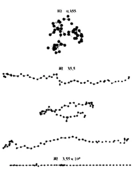
2-1 Sample chain trajectories in steady shear flow for N = 50 and We = 0.355,35.5, and 3.55x 108. Reproduced from Doyle et al. [16] .. . . . 21

2-2 Comparison of force-extension relationships for three springs force laws: Hookean (solid), FENE (dashed), inverse Langevin (dash-dotted line). The vertical dashed

line at Q/Qo = 1 corresponds to the maximum possible extension at which

nonlinear FENE and inverse Langevin forces diverge ... 23

2-3 Ways to incorporate molecular models into kinetic theory. ... 30

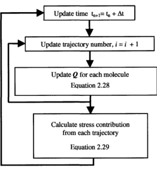
2-4 Forward Euler time integration algorithm for an elastic dumbbell ... 36

3-1 Evolution of the adaptive length scale L ...

42

4-1 6th order nonlinear algebraic function given by Equation 3.10 as a function of bsg. A value of boat = 150 was used to generate this figure ... 51

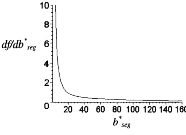
4-2 Plot of the first derivative of the function given by Equation 3.10. bma = 150. . 53 4-3 Timing comparison of various heological models ... 56

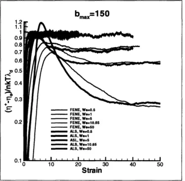
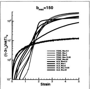
5-1 Transient polymer shear viscosity (+ - ,s)/lnkTAd for the FENE dumbbell and

the ALS models for bma = 150, Z = 1 and We = 0.5, 1, 5,10.65, and 50. FENE dumbbell results for We = 0.5 and 1 coincide with the ALS results for corre-sponding values of We ... 61

5-2 Transient poolymer elongational viscosity (7+-3r/)/nkTAd for the FENE dumb-bell and the ALS models for bmax = 150, Z = 1 and We = 0.5,1,5, 10.65, and

50 ... 62

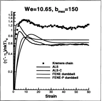
5-3 The dependence of M*eg on Q2 _{(made dimensionless by one-third of the} equilib-rium length of a FENE dumbbell) for various We. bmax = 150, Z = 1. ... 62 5-4 Dependence of transient polymer elongational viscosity on strain for a 50-rod

Kramers chain and the corresponding forms of the ALS, ALS-C, FENE dumbbell,

and FENE-P dumbbell models in start-up of uniaxial extensional flow for We

= 10.65. The maximum extensibility for the elastic spring models, bmax

is 150.

Kramers chain data are obtained from Doyle et al. [15]. ... 64 5-5 Dependence of polymer contribution to shear viscosity on strain for a 50-rod

Kramers chain and the corresponding forms of the ALS, ALS-C, FENE dumbbell,

and FENE-P dumbbell models in start-up of steady shear flow for We = 10.65.

The maximum extensibility for the elastic spring models, bmax is 150. bo = 150. Kramers chain data are obtained from Doyle et al. [15]. ... 65 5-6 Dependence of the first normal stress coefficient T+ on strain for a 50-rod

Kramers chain and the corresponding forms of the ALS, ALS-C, FENE dumbbell,

and FENE-P dumbbell models in start-up of steady shear flow for We = 10.65.

The maximum extensibility for the elastic spring models, bmax is 150. b = 150. Kramers chain data are obtained from Doyle et al. [15]. ... 66 5-7 Dependence of elongational viscosity on We for a 50-rod Kramers chain and

the corresponding forms of the ALS, ALS-C, FENE dumbbell, and FENE-P dumbbell models in steady elongational flow. The maximum extensibility for the elastic spring models, bmax is 150. Kramers chain data are obtained from Doyle et al. [16]. ... 67 5-8 Dependence of viscosity on We for a 50-rod Kramers chain and the corresponding

forms of the ALS, ALS-C, FENE dumbbell, and FENE-P dumbbell models in steady shear flow. The maximum extensibility for the elastic spring models, bmax is 150. bo = 150. Kramers chain data are obtained from Doyle et al. [16]. bo = 150. 68

5-9 Dependence of first normal stress coefficient on We for a 50-rod Kramers chain

and the corresponding forms of the ALS, ALS-C, FENE dumbbell, and FENE-P

dumbbell models in steady shear flow. The maximum extensibility for the elastic spring models, bma,,x is 150. Kramers chain data are obtained from Doyle et al.

[16]. bo = 150 ... 69

5-10 Polymer stress vs. birefringence for start-up of elongational flow up to E = 6

and subsequent relaxation. The results are shown for the Kramers chain with

N = 50, the ALS, ALS-C, FENE dumbbell, and FENE-P dumbbell models with

bmax = 150. Kramers chain data are obtained from Doyle et al. [17]. ... 71 5-11 Sample chain configurations during start-up of extensional flow at We =10.65

and subsequent relaxation. During start-up the chain follows the right hand side

path, and the left hand side path is followed during relaxation. Reproduced from

[17]

...

...

71

5-12 Dependence of polymer contribution to the elongational viscosity on strain in the ALS model for values of Z = 0.1, 0.2,0.5, 1,2,5, 10. We = 10.65 and bmax = 150

are held constant. . . . ... 72

5-13 Dependence of polymer contribution to shear viscosity on strain in the ALS model for values of Z = 0.1, 0.2, 0.5, 1, 2, 5, 10. We = 10.65 and bmax = 150 are held constant. bo = 150 ... 73 5-14 Dependence of the maximum number of segments Mseg,max on Z for uniaxial

elongational flow at We = 10.65 and bma = 150. ... 74 5-15 Dependence of the maximum number of segments Mseg, max on Z for simple shear

flow at We = 10.65 and bm,, = 150. ... 74

5-16 Dependence of transient polymer viscous stress growth coefficient qr+ on strain for a 50-rod Kramers chain and the corresponding forms of the ALS, ALS-C, FENE dumbbell, and FENE-P dumbbell models in start-up of steady shear flow for We = 10.65. The maximum extensibility for the elastic spring models, bmax,

is 150. ... 75

6-1 Linear viscoelastic fit to the experimental data by Rothstein [49]: (a) single-mode fit, (b) 4-mode fit. ... 77

6-2 Single-mode data-fitting to experimental data in order to find the best value of

b,.

The included results are: i) experimental data with 0.025 wt% PS solution

([49]), simulation results with a single-mode ALS model with Z = 0.25,0.5, 1 and 2, and simulation results with a single-mode FENE dumbbell model. (a)

bmax = 7744, (b) bmax = 1000, (c) bmax = 500, (d) bmax = 1000. Trouton ratio

is defined as +/,r0, where r/+ is the transient extensional viscosity and r0 is the zero-shear-rate viscosity; = 9.1 sec ... 79 6-3 Data fitting to extensional rheology with (a) 4-mode ALS model and (b) 4-mode

FENE dumbbell model to determine the best values of bma,, for each mode. Trouton ratio is defined as V+/r0o, where A+ is the transient extensional viscosity

and r70 is the zero-shear rate viscosity. The vertical dashed line at Strain of

2.75 indicates the maximum value of strain achieved in the experimental setup;

= 9.1 sec . . . ... . 80

6-4 Dependence of polymer elongational viscosity on strain for a 50-rod Kramers chain and the corresponding forms of the ALS, FENE dumbbell, 5-mode FENE

dumbbell and the 5-spring FENE chain models in start-up of uniaxial extensional

flow at We = 10.65. The maximum extensibility for the single-mode ALS and the single-mode FENE dumbbell models, bma,, is 150. The maximum extensibility for each mode of the 5-mode FENE dumbbell model, starting from the slowest one, are: 150, 75, 50, 37.5, and 30. Maximum extensiblity of each spring in the chain is 30. Kramers chain data are obtained from Doyle et al. [15]. Insert: Dependence of the ensemble-averaged number of segments in the ALS model on

strain

...

...

81

7-1 Comparison between Lagrangian (CONNFFESSIT) and Eulerian (Brownian

con-figuration fields) implementations. (a) Lagrangian implementation, in which en-sembles at adjacent nodes are uncorrelated; (b) Eulerian implementation, where the same ensemble of random numbers is generated at each node in the physical

7-2 In the operator splitting method, the macroscopic process environment solver and

the microstructure solvers are completely decoupled, which means that changes to one of the solvers have no effect on the other one. ... 88 7-3 Schematic of the parallelization process for the contraction-expansion problem. . 90

7-4 Schematic of the contraction-expansion geometry. R

1

is the radius of the

up-stream

...

91

7-5 Extra pressure drop made dimensionless by the pressure drop for the Newtonian

fluid as a function of De for the 4:1:4 axisymmetric contraction-expansion

prob-lem with a sharp re-entrant corner. Data presented are from experiments ([48])

and from computations with the FENE-CR model with the maximum

extensibil-ity L =- 3.2, 4, 5 ([56]). The horizontal dashed line corresponds to the Newtonian

limit

...

92

7-6 Extra pressure drop made dimensionless by the pressure drop for the Newtonian

fluid as a function of De for the 4:1:4 axisymmetric contraction-expansion

prob-lem with a rounded re-entrant corner. The plot includes: experimental data for

the Boger fluid by Rothstein and McKinley ([49]), FENE-P dumbbell results and

single-mode ALS-C results with Z = 0.25, 0.5, 1, and 2 and bmax = 7, 744 from simulations by Phillips ([47]) ... 93

7-7 Flow past a linear, periodic array of cylinders confined between two parallel

plates. The cylinders each have radius R,, and the geometry is specified by the

cylinder-to-cylinder spacing L and the channel half height Hc. The unit cell on

which computations are performed is shaded. ... 94

7-8 Dependence of the critical Weissenberg number, Wecr on the inter-cylinder

spac-ing L for the flow around an array of cylinders confined between two parallel plates. Data presented are: PIB/PB Boger fluid experimental data by Liu ([38]), simulation results with an Oldroyd-B model by Smith et al. ([50]), and

simu-lations results with the ALS-C model by Joo et al. for ba = 120 and 12,500

List of Tables

2.1 Comparison of the Fokker-Planck and the stochastic approaches in solving vis-coelastic flow problems. ... ... 37 4.1 Breakdown on timing for the ALS and the FENE dumbbell models ... 56 6.1 Set of parameters for a 4-mode ALS model resulting in the best fit to the transient

uniaxial elongation experimental data of Rothstein et al ...

78

7.1 Operation count for the ALS model in complex flow calculations ... 88

Chapter 1

Introduction

1.1 Motivation

Polymers are a large class of materials consisting of many small molecules called monomers that are linked together to form long chains. A typical polymer may include tens of thousands of monomer units. Because of their large size, polymers are classified as macromolecules. Polymers can be found occuring in nature, and they can also be made synthetically. Arguably, the most important natural polymer is DNA, which is a genetic blueprint that difines all living things. People have taken advantage of the versatility of polymers in the form of oils, resins and tars

for hundreds of years, but the modern polymer industry began developing during the Industrial

Revolution. However, the progress in polymer science was relatively slow until the 1930's when polymers such as vinyl, neoprene, polystyrene, and nylon were invented. Today, natural and synthetic polymers are used in nearly every industry due to the unmatched diversity of their properties such as strength, heat resistance, stiffness and density.

Because of their long-chain architecture, polymers, which fall into the category of non-Newtonian fluids, tend to exhibit behavior that is different from their non-Newtonian counterparts. In particular, non-Newtonian fluids exhibit shear rate-dependent viscosity and non-zero normal stresses in simple shear flow and elongation rate-dependent extensional viscosity in simple elongational flow. These fluids may also display time-dependent effects, with the fading memory of the polymer given by a characteristic relaxation time A. Some striking flow phenomena are

summarized in Figure 1-1: (a) In a tubeless siphon experiment, a fluid gets siphoned out of a container when a tube is lifted. While a Newtonian fluid will stop flowing, a non-Newtonian fluid will continue to flow, (b) In a die-swell experiment, a polymeric fluid exits a capillary with

the diameter of the exiting jet increasing to about 300% of the capillary diameter. In contrast,

a Newtonian fluid would have a die-swell of no more than 13%, (c) When a non-Newtonian fluid is stirred with a rod, normal stresses create tension along the circular lines of flow, thus causing

the fluid to climb up the rod. This is called the "rod climbing" or the Weissenberg effect. Other

phenomena such as secondary flow, jet break-up and elastic recoil are depicted and explained

in [4] and [9].

0_

L

(b) (C)

Figure 1-1: Non-Newtonian fluid flow phenomena. (a) Tubeless siphon; (b) Die-swell; (c) Rod

climbing. [4]

The non-linear behavior of non-Newtonian fluids lies in the origin of the fundamental prob-lem in polymer fuid mechanics of how to calculate the stress tensor, which in itself is a function

of various kinematic tensors. In the case of a Newtonian fluid, the stress tensor is linearly

proportional to the velocity gradient and is given by the Newton's law of viscosity, but no

such unique constitutive equation exists for non-Newtonian fluids. Over the years, a number of

empirical relations have been proposed to calculate polymer contribution to the stress tensor,

and they are reviewed by Bird and Wiest [8].

In order to predict accurately a polymer's heological properties, it is important to have a

good understanding of the various conformations that a polymer molecule may assume, and ideally, the forces along its backbone in a variety of flow situations. A homogeneous, or simple, flow falls into a class of flows in which the velocity gradient tensor, which describes the kine-matics of the fluid, does not vary spatially. Common types of simple flows are shear, uniaxial elongational. and planar elongational flows. One of the major challenges of the polymer kinetic

theory on the experimental front has been to understand the relationship between the

config-uration of an individual molecule and the force along its backbone. Such understanding could be used to design a micro-mechanical model whose backbone forces were related to conforma-tion at a submolecular level, the same way it is for actual polymer molecules. A variety of experimental techniques have been used to gain this understanding. These techniques include optical methods such as birefringence and light scattering, which provide information about the mean orientation and conformations of the molecules, nuclear magnetic resonance (NMR)

and neutron scattering methods, which provide detailed information about the conformational

distribution function, and fluorescence video microscopy, which provides direct observations of molecular conformational changes in the flow [54]. An important milestone was the develop-ment of a filadevelop-ment stretching rheometer, which allowed for quantitatively reliable measuredevelop-ments

of transient stress growth as a function of strain and strain rate in uniaxial elongational flows

[57].

Experimental advances in birefringence measurements have also allowed for a better un-derstanding of the average molecular conformations in complex flows. Techniques which can visualize the birefringence at every point in a complex flow were developed by Liu [38], Geneiser [22], and Burghardt et al. [11]. Birefringence is related to the second moment of the

config-urational distribution function and can therefore yield information about the conformation of

molecules in the flow domain. By using the stress-optical rule, which predicts a linear

re-lationship between stress and birefringence, the researchers claimed that their birefringence

measurements can be used to calculate polymer contribution to the stress in the entire flow

domain. However, Doyle et al. later showed that the stress-optical rule breaks down for large strains in elongational flows [17]. In addition, the stress-optical relationship was found to vary with the flow history experienced by the polymers. Hence, birefringence measurements can

provide only limited information about the stress field in a complex flow geometry.

Molecular models are used in kinetic theory because they can provide information about the conformations of polymer chains in solution, which is of great importance for accurate prediction of the final product properties. Aside from that, the use of molecular approach is important for a number of other reasons. Polymeric liquids are usually composed of chains with different molecular weights, and this polydispersity can have significant effects on the fluid's rheology. Information provided by molecular models such as molecular architecture and chain stiffness can be used to improve existing models. The use of molecular models can also help account for solvent-solute interactions as well as elucidate the behavior of viscoelastic fluids near

boundaries such as sharp corners, contact lines and stagnation points. The ultimate goal is to

connect the information provided by molecular modeling with the macroscopic calculations to solve industrially important problems such as fiber spinning, film blowing and injection molding.

1.2

Viscoelastic flow analysis

The first step in understanding non-Newtonian fluids lies in being able to characterize them properly. For example, Newtonian fluids at constant temperature can be characterized by just

two material constants: the density p and the viscosity

ji.

Once these properties have been

measured, the governing equations for the velocity and stress distributions in the fluid are fixed for any flow system [4]. On the other hand, experiments performed on non-Newtonian polymeric fluids yield a number of material properties, which may depend on shear rate, frequency, time, etc. The two standard kinds of flows used to characterize polymeric liquids are shear and

shearfree flows, which are discussed in detail in [4] and are briefly summarized here. The velocity field for a simple shear flow is given by

Vx = ,y; V = ; V = (1.1)

where the velocity gradient · yx can be a function of time. The magnitude or the second invariant of the rate of strain tensor

4

= Vv+ VvT is called the shear rate .y, and it is independent of time for steady shear flows. Simple shear flow is completely characterized by three material functions, which for steady state are the viscosity qr, and the first and second normal stress

coefficients ii and 2. These material functions have the following definitions

Tyx = -7)yzx (1.2)

7:rx-Tyy

=

-l()

s

(1.3)

Tyy - Tzz = -I_2(Y)2 (1.4)

Simple shearfree flows are given by the velocity field 1

Vx = -

(1 + b)x

(1.5)

2

y = -&(1 - b)y (1.6)

sr = $+-z

(1.7)

where 0 < b < and

E

is the elongation rate, which can be time-dependent. The choice of the

parameter b determines the type of a shearfree flow

Uniaxial elongational flow: (b = 0, E > 0) Biaxial stretching flow: (b = 0, E < 0) Planar elongational flow: (b = 1)

For steady simple shearfree flows, there exist two material functions, ]1% and /2, which define

two normal stress differences

Tzz - X = - 1(, b)& (1.8)

Ty-AXX =

-2

2

(E,b)i

(1.9)

If the flow is uniaxial elongational, 2 = O and /1% is defined to be the elongational viscosity

The three most important dimensionless parameters that govern the flow of non-Newtonian fluids are the Reynolds number (Re), the Deborah number (De), and the Weissenberg number (We). The Reynolds number is defined as the ratio of inertial forces to viscous forces, and due to high viscosities of polymeric liquids, this parameter is typically negligible and hence Re 0 is assumed in most calculations.

The Deborah number is defined to be the ratio of the polymer characteristic relaxation time

A to the observation time, T, i.e. De = A/T. The observation time is typically the residence time of a polymer molecule in the flow process. If De < 1, polymer molecules relax very quickly and the fluid is essentially Newtonian. In the case of De > 1, molecules are not able to change their configuration at all on the time scale of the flow, and the fluid behaves like a Hookean elastic solid. The most interesting phenomena, such as those depicted in Figure 1-1 can be observed when De 1, in which case the fluid is called viscoelastic.

The Weissenberg number is defined as the product of the characteristic polymer relaxation

time and the characteristic strain rate r, i.e. We = A. In many flow geometries, the

charac-teristic time of the flow is the inverse of the characcharac-teristic strain rate, in which case De and We can be used interchangeably.

1.3 Commonly used constitutive equations

Until very recently, the traditional approaches used by chemists, engineers and polymer physi-cists for deriving constitutive equations for stress calculation have been based on either simple mechanical models (e.g. convected Maxwell model), or on using engineering correlations (e.g. Carreau viscosity model for shear-thinning fluids) or mathematical expansions around New-tonian solutions (e.g. retarded motion expansion). Because each one of these approaches applies to a narrow class of flows, improper use of continuum-based models can lead to erro-neous results. Chapter 2 will explain the merits of molecular-based models and information they provide.

1.4 Thesis goals and outline

The main goal of this thesis is to develop robust, accurate methods to capture fine-scale polymer

dynamics in simple flow calculations. The particular research directions for achieving this goal were:

1. Optimization of the Adaptive Length Scale model (ALS), which was originally introduced by Ghosh et al. [25], in order to have the simulation time as close as possible to that of a FENE dumbbell. Such optimization is necessary because complex flow simulations employing the use

of Brownian dynamics are expensive with the majority of CPU time spent on generating random

numbers and calculating stress (see Chapter 7).

2. Assessment and comparison of the ALS model with other competing rheological models in simple flows to find a balance between the wish to have as detailed a model as possible and the ability to simulate it in a reasonable amount of time.

3. Evaluation of the use of multi-mode models to capture the range of time scales caused by polydispersity in a real polymer solution.

4. Assessment of closure approximations on the physics predicted by a given model. And the final goal was to evaluate the feasibility of using the Adaptive Length Scale model in complex flow calculations by doing an operation count. As discussed in Chapter 7, the closed-form of the ALS model, called ALS-C, yields certain predictions in the contraction-expansion geometry as well as in the flow around an array of cylinders confined between two parallel plates, which are missed by the FENE dummbell model. Therefore, it is of great interest to determine how the unapproximated version of the model will behave in the same flow situation.

The thesis is organized in the following way. Chapter 2 introduces and reviews the kinetic

theory of polymers. The chapter begins with the introduction of various micromechanical models used to represent polymer molecules. Then, three different approaches for incorporating

molecular models into stress calculations are discussed, followed by a brief summary of the

techniques to reduce noise in a Brownian dynamics simulation. Chapter 3 introduces the

Adaptive Length Scale (ALS) model, which was designed to capture the fine-scale dynamics of a Kramers chain while retaining only one more degree of freedom in addition to what a simple

FENE dumbbell possesses. This chapter discusses the qualitative and quantitative aspects of

the model, and it also summarizes the governing equations for a closed-form version of the model, ALS-C proposed in [25]. The focus of Chapter 4 is to describe the approaches that were taken to optimize the ALS model so that its simulation time would be as close as possible to that of a FENE dumbbell. One of the governing equations in the ALS model is a 6th degree nonlinear algebraic equation for the instantaneous maximum extensibility of a segment, b*eg. The solution of this equation is extremely time-consuming, and therefore different approaches

such as the bisection method, the Newton's method, lookup table, etc. were evaluated and

compared to determine which method gives the fastest solution without a sacrifice in accuracy.

The chapter concludes with a discussion of the relative merits of explicit and semi-implict time-integration techniques. Chapter 5 is devoted to presenting the rheological predictions of the ALS model in transient as well as steady simple shear and uniaxial elongational flows. This chapter is concluded by examining the model's parameter dependence. Since most real polymeric solutions contain chains of different molecular weights and hence different contour lengths and relaxation times, the use of multi-mode models in explored in Chapter 6. Chapter 7 focuses on the use

of stochastic methods in complex flow calculations. First, the CONNFFESSIT (Calculation

of Non-Newtonian Flow: Finite Element and Stochastic Simulation Technique) approaches

based on the Lagrangian and the Eulerian point of reference are presented. In the former,

the location of each stochastic trajectory representing a polymer molecule is tracked by an ordinary differential equation. In this approach, which was introduced by Laso & Ottinger [31],

the stochastic trajectories at adjacent nodes are not correlated, which means that Nnode * Ntraj

random numbers have to be generated, where Nnode is the number of nodes in the spacial

discretization and Ntraj is the number of stochastic trajectories being simulated. The Eulerian

approach, which is also called the Brownian Configuration fields technique, was introduced by Hulsen et al. [26] and van den Brule et al. [58]. By replacing individual stochastic particles by continuous configuration fields, they achieved a two-fold benefit. First, because fields at adjacent nodes are correlated, only Ntraj random numbers need to be generated, where Ntraj is now the number of convected configuration fields, which results in an enormous computational time saving. And two, this correlation results in a natural variance reduction, thus decreasing the noise of the simulation. The rest of the chapter is devoted to performing an operation count on the ALS model to show that the model is feasible for use in complex flow calculations on parallel processors. The chapter is concluded by showing complex flow results of the ALS-C

model, which explain its advantage over the commonly used FENE-P dumbbell model. The

main findings of this thesis and suggestions for future work are summarized in Chapter 8.

Chapter 2

Introduction to Polymer Kinetic

Theory

It is often of interest in materials processing to know not only the velocity and stress fields, but also the molecular configurations and orientations. To obtain the latter, one usually begins by proposing a model of the molecular structure. Given the fact that computing the elec-tronic structure of each atom within a polymer molecule using ab initio molecular dynamics

is impractical for calculating transport and thermodynamic properities, most micromechanical

models are constructed using classical mechanics. These micromechanical models can in gen-eral be divided into two types: (1) particle-based discrete models, which are used for modeling dilute solutions and will be discussed in this thesis, and (2) field-theoretical continuous models,

which are generally used to model concentrated polymer solutions and melts. Then one solves

self-consistently the governing microscopic and macroscopic equations. Ideally, the proposed

molecular model would be as detailed as possible in order to capture maximum number of

im-portant aspects of a real polymer molecule. The problem, however, lies in the fact that a typical

polymer chain has a broad spectrum of time scales. The shortest ones are related to molecular

vibrations and are roughly of the order of 10-12 seconds, whereas the slow modes can be of the order of 10 seconds or longer. This kind of spectrum would clearly be impossible to model, and for that reason, a common practice in the polymer kinetic theory has been to focus only on the slow processes that govern the global configurations of the macromolecules by studying

the response of coarse-grained models. Bead-spring and bead-rod chains are commonly used as such models. A detailed account of various coarse-grained models can be found in [5] and [7]. The coarse-grained models are generally nonlinear and possess a large number of degrees of freedom, which complicates their simulation even in simple flows.

2.1 Micromechanical models

The most commonly used molecular models, beginning with a relatively fine-grained one known as the Kramers chain, will be discussed in this section, followed by a discussion in the next chapter of the recently proposed single-mode Adaptive Length Scale model (ALS), which takes into account kinematic history of the flow and is able to capture the fine-scale physics of the Kramers chain without having the high computational cost associated with simulating the

latter.

2.1.1

Bead-rod chains

A Kramers chain, or a freely-jointed bead-rod chain, consists of N beads joined together by N-1 massless rods. The beads do not represent individual atoms of a polymer chain, but rather a collection of atoms along the molecule's backbone. Each rod has a constant length a, which corresponds to a Kuhn step ([21]). The name 'freely-jointed' comes from the fact that the rods are allowed to move freely about beads and do not experience bending potentials. Beads and rods can also move 'through' one another, because excluded volume is not accounted for in this model. Solvent molecules are modeled as a continuum, which is described by an incompressible Newtonian liquid with viscosity rs. In the absence of body forces, each bead v is subjected to three forces, namely (1) the hydrodynamic drag force F(h) imparted by the solvent, (2) the

Brownian motion force F

(

B), which results from the bombardment of the beads by the solvent

molecules constantly undergoing random thermal motion, and finally (3) the constraint force

FC( ), which arises from tensions in the rods. Definitions of each of the three forces as well as the force balance can be found elsewhere ([45],[24]). From simulations of Kramers chains in relaxation following the cessation of uniaxial elongational flow, Doyle et al. ([16]) found that the longest time scale, Ad, of the polymer is related to the diffusive time for a single link

(r\od

=

Ca

2

/kT) by

Ad = 0.014 2N2 a (2.1)

where ( is the bead drag coefficient of the Kramers chain, k is the Boltzmann constant, and T

is the temperature. In dimensionless form Equation 2.1 has the following form

We = 0.0142N2Pe (2.2)

The dimensionless group Pe, which naturally arises in Equation 2.2 is the Peclet number, which is the dimensionless diffusion time defined as

a2

Pe = T

(2.3)

Here, is the extension rate, and the Weissenberg number in Equation 2.2 has the following definition, We= Ad. The expression for the birefringence ([16]) is

N-1

An = 5CnkT y

(uzuVz

-

:uxU)

(2.4) I=1 where

C =

45kT

2)2 2) (2.5)

45kT

n

and n is the isotropic part of the refractive index tensor, (al, a2) are the (parallel, perpendicular) components of the polarizability tensor, and (UVX, uL) are the (x, z) components of the unit

vector pointing from the vth to the (v + 1)th bead.

Liu [39] established the first numerical method for performing Brownian dynamics simula-tions of dilute solusimula-tions of Kramers chains. The condition of constant length of each link in the chain was imposed in his algorithm through the use of Lagrange multipliers. By studying polymer molecules at sudden inception of elongational flows, he was able to obtain visualiza-tions of the chain-unfolding mechanism during the coil-stretch transition. In general, a Kramers chain would have to have on the order of 1000 or more beads in order to mimic a real polymer molecule. But since this kind of simulation is not feasible with current computational resources, researches have modeled chains of 50-200 beads in order to compare their results to the

exper-imental observations. Simulations of a Kramers chain in the start-up of shear and extensional flows as well as comparison of the results to experimental data can be found in [15]. Doyle et al. ([16], [15]) showed that a Kramers chain is capable of exhibiting internal configurations such as kinks and dumbbells similar to those of a real polymer molecule undergoing shear and elongational flow (see Figure 2-1). The study of the rheological and optical behavior of Kramers chains by using stochastic methods in steady shear and uniaxial extension is described in [16].

The authors also developed an algorithm to split the stress into its Brownian and viscous

con-tributions. Based on the algorithm proposed by Liu [39], Ghosh et al. [24] analyzed Kramers chains in uniaxial elongational flows in order to understand the fine-scale physics that the chains are capable of capturing and to assess the validity of coarse-grained models. Both, Doyle et al. [17] and Ghosh et al. [24], showed that besides exhibiting the distributional stress-birefringence hysteresis, a Kramers chain also exhibits residual hysteresis, which Doyle et al. termed the configuration hysteresis. It arises because molecules tend to assume different configurations during extension and relaxation. Most synthetic polymers such as polystyrene, polyethylene, and polypropylene are flexible molecules, which can be represented well by the Kramers chain. A Kramers chain is a relatively detailed model which can accurately represent the important dynamics of a real molecule, but its many degrees of freedom do not allow it to be used in complex flow calculations. Hence, further coarse-graining is required.

2.1.2

Elastic chains

To make problems computationally tractable, dilute solutions of polymer molecules are often modeled as beads connected by springs. These bead-spring chains are coarsened versions of the Kramers chains, many segments of which are represented by a single spring, whose "effective" force is entropic in origin. While this is the representation used by most researches, Laso et

al. [32] showed that such coarse-graining will result in non-uniform bond and torsional angle

distribution, thus preventing the bead-spring model from being truly freely-jointed. Thus, even

though both the bead-rod and the bead-spring chain models provide detailed information about

polymer microstructure, there does not exist a unique mapping relationship between the two.

The bead-spring chains are suspended in a Newtonian solvent and are convected and dis-torted by the viscous forces exerted on the beads. The beads also experience a randomly

Ii? I.Afs

i . .55

f ,* 4 .7.. ki,. -' ~ee.a~ ' me w·oe' '~'~,. -a'-o? '.. . . ·. *f M A.55w IIt,, dW-d,e -. ,,- o s e ., , *+---,,- -- . - -+ - , r- ,+

Figure 2-1: Sample chain trajectories in steady shear flow for N = 50 and We = 0.355,35.5, and 3.55x 108. Reproduced from Doyle et al. [16]

fluctuating force due to the thermal agitation by the surrounding solvent molecules, the

so-called Brownian force. The hydrodynamic and Brownian forces have the same form as for the Kramers chain. However, unlike the Kramers chain, no constraints exist in an elastic chain, which reduces the simulation time tremendously.

A widely used model for dilute polymer solutions is the Rouse chain, which is made up of beads joined together by Hookean springs. The Hookean force law is given by

F(c)(Q) = HQ

(2.6)

In this equation, F(c) is the connector force, H is the spring modulus, and Q is the

end-to-end vector representing a particular spring in a chain. The constitutive equation associated

with this Hookean chain is, in fact, identical to the macroscopic multi-mode Oldroyd-B model. The Rouse chain model is well understood and, because of its linearity, is often amenable

to analytical solutions. Major shortcomings of the Rouse chain are that none of the steady

shear flow material functions obtained using this model depend on the shear rate and that

the springs in the chain can be stretched indefinitely. This can lead to an unbounded value

of the elongational viscosity at high strain rates. All of these results are in disagreement with

experimental data.

It is suggested in [5] through the use of kinetic theory that the force law for polymer chain models should be nonlinear in the extension of the spring, Q. The most commonly used nonlinear force law, Finitely Extensible Nonlinear Elastic (FENE) spring force law has the following form:

F(C)(Q)

=

HQ

(2.7)

1-The FENE force law is an approximation to a more complicated inverse Langevin force law proposed by Warner [62] and is derived based on the equilibrium force-extension relationship for a Kramers chain. The Langevin force law is in given by

F (c)(QQ)

= Ho_

(2.

(2.8)

addition, L-lin Equation 2.8 is the inverse Langevin function given by L(x) = coth(x)

-

x

- 1

.

A comparison between the inverse Langevin, FENE and Hookean force laws is given in Figure

2-2.

Figure 2-2: Comparison of force-extension relationships for three springs force laws: Hookean (solid), FENE (dashed), inverse Langevin (dash-dotted line). The vertical dashed line at

Q/Qo = 1 corresponds to the maximum possible extension at which nonlinear FENE and

inverse Langevin forces diverge.

As can be seen in Figure 2-2, the three force laws yield identical results for small extensions

(Q/Qo < 0.5). For larger extensions, the Hookean force law, which is a linear approximation

to the inverse Langevin force law, underpredicts the spring force. The FENE force law, on the

other hand, is a good approximation to the inverse Langevin force law for the whole range of

Q/Qo. An important feature of these two force laws is that the forces they predict diverge for

dimensionless extensions close to unity, which is designed to mimic a real polymer molecule with a finite extensibility. One of the major problems with Hookean springs is that they can be stretched indefinitely, which is clearly aphysical. A major drawback of a FENE chain is that it

does not allow for a closed-form constitutive equation for the polymer stress, and therefore it

is not suited for traditional continuum approaches to numerical solution of complex flows. As discussed later on in the thesis, this problem can be avoided by coupling direct simulation of a molecular model with solution of the conservation equations from fluid mechanics.

16 .14 p 10 O 1 8 .2_o .C 6 C0 4 C

0 ,

A

12--

Hookean

it

- -- FENE i1 -.-- - Langevin i I 0I a! I u! I i! I .'

*!

$,,'J

v0 0.2 0.4 0.6 0.8 1 1.2

To circumvent the closure problem in the macroscopic finite element calculations, a

mod-ification of the FENE model with a Peterlin approximation, which constraints the average

extension of the j segments to a maximum value of Qo, was introduced. The force law for a link in a chain of FENE-P springs has the following form

Fj (Q)

HQ=

j = 1..N- 1

(2.9)

1-(Q2)/Q

2'

Because with this model the system of equations governing the evolution of the second

moments cannot be transformed to normal coordinates, the calculation involves solving an

N-1 by N-I matrix of 3-dimensional tensorial differential equations, where N is the number of beads in the chain. Rigorous solutions for a FENE-P chain in shear flow are provided in [44], [64], and [66]. The number of equations to be solved in this model increases roughly as N2,

and the problem can become computationally expensive even for a relatively small number of beads. Bird et al. [6] attempted to decouple their constitutive equation, but made an error

in transformation to normal coordinates. Therefore, the constitutive equation they obtained is

not that; for a true FENE-P chain, but rather for an empirical multimode model that contains

time constants which depend on a transformation matrix.

A modification of the FENE-P model called FENE-PM is proposed in [63]. The authors

replaced the denominator of the FENE-P spring force with an expression that is invariant under

the transformation to normal coordinates. The FENE-PM expression has the form

F' (c )=

(HQj

(2.10)

Ff)(Q) : N-1

11

ZK1

E

Q/Q0)

2 )

j=1

This form of the force law constrains the arithmetic average of the square of the average end-to-end distances of the links to the square of the maximum extension Qo. One downside of the FENE-PM model is that it is possible for one link in the chain to have (Q2) (N 1) QO, with all other (Q2) . However, as shown in [63], this situation does not occur in shear and elongational flows. After introduction of normal coordinates, the number of FENE-PM second moment equations that need to be solved is proportional to N - 1, which is a significant

reduction from the number of equations in the FENE-P model. FENE and FENE-P models

in start-up of shear and uniaxial elongational flow are compared in [60]. Because closing a model can sometimes significantly alter results of the calculations, the authors offered ways to

select parameters of the FENE-P model such that the important FENE flow characteristics

are not lost. The effects of excluded volume, polymer chain length, maximum bond extension,

and hydrodynamic interactions of the FENE model in steady and transient elongational flows,

obtained by using Brownian dynamics simulations, and comparison of the results to the analytic FENE-PM theory of Wedgewood et al. [63] are presented in [20]. The problem with closure approximations as applied to FENE dumbbells was also addressed in [29] and [58].

The birefringence of bead-spring models can be calculated using the expression from [65] as

M

An =

5CnkT --

E

(izi

z

QxQix)

(2.11)

where C is given by Equation 2.5, M is the number of springs, Qso is the maximum extension

of a spring and each spring corresponds to ns rods in the Kramers chain representation of a

polymer molecule.

2.1.3

Dumbbells

As in the case of the Kramers chain, FENE chains have too many degrees of freedom to be used in complex flow calculations. The most commonly used molecular models in fluid mechanics calculations are the elastic dumbbell models, in which polymer molecules are represented by two beads joined together by a linear or a nonlinear spring. The elastic dumbbell model is usually used to represent the end-to-end vector of a Kramers chain. The inverse Langevin force

law (and the FENE approximation to it) is obtained from equilibrium statistical mechanics

and is based on the assumption that for a given end-to-end distance a Kramers chain has had

sufficient time to sample its entire configuration space and that the internal conformational

distribution has reached equilibrium. This force law should be used with caution in non-equilibrium situations when molecules are undergoing rapid stretching. The chain will unravel

reversibly only when the time scale of the deformation is much longer than the relaxation time

scale of the entire chain, i.e. the internal conformation of the chain will be able to equilibrate at each stage of the stretching ([23]). Similar to the Kramers chains, FENE dumbbells exhibit

distributional hysteresis, but they lack a sufficient number of internal degrees of freedom to

have configurational hysteresis. The time constant, Ad, for a FENE dumbbell is

Ad =

(d/

4_{Hd (2.12)}

where the dumbbell spring modulus

Hd

is related to the Kramers chain parameters through

the following equation

Hd=

3kT

(2.13)

(N - l)a

2

Combining Equations 2.1, 2.12, and 2.13, we can obtain a relationship between the bead drag

coefficient of the Kramers chain and that of the FENE dumbbell,

(d,

N

2

(d = 0.1 7 0 4 - (2.14)

There is no unique way to match the time constant for a dumbbell to the time constant

of an individual spring in a bead-spring chain. The scaling relationship chosen by Ghosh

[23] is such that the transient extensional viscosity of the FENE chains approaches the profile

predicted by the Kramers chain as the number of springs in the chain M becomes large. This

condition can be satisfied by a scaling relationship that makes the zero-shear-rate first normal

stress coefficient independent of M. Using the result for the zero-shear-rate first normal stress

coefficient presented by Van den Brule et al. [58] gives the relationship between the time

constants as

A,-

C

8 _ Ad (2.15)

4H

K

where K is given by

K

b

8

(bmax+5)(bmax+7)

[2(M + 1)

2

+ 7]

[(M

+

1)

2

-1]

12

[(M

+

1)4

-1]

1/2

b + 5

bmax

45

45(M + 1)(b + 7)

(2.16)

polymer molecule is represented by a single dumbbell, which is defined as

HdQ2

bmax kT (2.17)

kT

bs

is the maximum extensibility of spring in a bead-spring chain defined by

HdQ2

bs =MT (2.18)

MkT

The quantity bmax

is related to the number of rods in the Kramers chain through the following

expression

bmax

= 3(N - 1)

(2.19)

While there is no unique way of matching the parameters in the Kramers chain, the FENE

chain, and the FENE dumbbell models for proper comparison of their results, if one is interested in studying systems far away from equilibrium, the following matching technique can be used:

(1) Set the time scale

Ad

of the dumbbell to the slowest relaxation time of the Kramers

chain and

(2) Use the scaling relationship given by Equation 2.15 to match the time scale of the

dumbbell to that of an individual spring in the chain.

Doyle et al. [16] showed that the Kramers chain and the FENE dumbbell cannot predict the same values for the following pairs of properties if the FENE dumbbell has a constant drag coefficient: (1) the zero-shear-rate viscosity and zero-shear-rate first normal stress coefficient and (2) the steady-state elongational viscosity at zero and infinite elongation rate. In order to match the zero-shear-rate viscosities of the two models, they chose the bead drag coefficient

for the FENE dumbbell to be (2/3)NC. With this choice, the FENE dumbbell predicts the

zero-shear-rate first normal stress coefficient to be twice that of the Kramers chain.

Whereas the FENE model and its closed versions have been the most popular nonlinear elastic dumbbell models, a new kind of model, termed a HYBRID model was proposed in [12]. The HYBRID model consists of springs that are Hookean at low elongations until the spring length Q reaches some critical value Qc, after which they follow a Morse potential with a given dissociation energy. This new model was shown to be suitable for studying polymer fracture in

strong flows. In trying to develop a closed model that would be capable of reproducing the stress vs. mean square extension hysteresis displayed by the FENE model, Lielens et al. [36] proposed a more sophisticated second order closure model for one-dimensional flows, which they referred

to as FENE-L. This model approximates the distribution function as a composite of a delta

function and a rectangular element. The addition of the rectangular segment adds dispersity to

the distribution function. In a follow up paper, Lielens et al. [37] extended the model to general,

three-dimensional flow kinematics. The authors reported simulations for steady and transient

rheometrical flows, which demonstrated the superiority of the FENE-L constitutive equation

with respect to the classical FENE-P closure in describing the response of the FENE dumbbell

model, both in shear and elongational flows. In particular, the FENE-L model was able to predict the stress-birefringence hysteresis, which is out of reach for a single-mode FENE-P

dumbbell.

Dumbbells are by and far the least expensive models to use in finite element calculations,

but because they only have three degrees of freedom, the three components of the

end-to-end vector Q, they perform poorly in predicting experimentally observed behavior of polymer solutions in the start-up of extensional flow [15], [24]. In particular, it is demonstrated in [24]

through simulations of the Kramers chain, that for a given value of the end-to-end distance,

the effective force in a polymer molecule varies with strain and strain rate. In contrast to this

observation, the FENE force law, which describes the entropic elasticity in a slowly stretching polymer chain, is not dependent on either quantity. It is also shown in [25] that whereas a short

FENE chain is needed to describe stress growth at low strains, a FENE dumbbell would suffice

at higher strains when the molecules are almost fully unraveled. Therefore, the use of a FENE

chain with its many degrees of freedom would not be the most efficient way to model a polymer molecule under varied flow conditions. To avoid the problem of having to map between FENE chains with different numbers of springs, Ghosh et al. proposed a new single-mode constitutive equation, which they termed the Adaptive Length Scale (ALS) model. The ALS model is

described in the next chapter.

2.2 Incorporating molecular models into stress calculation

One of the goals of a microscale simulation is to get an expression for the tensor (QQ), which is the ensemble average of the dyadic product of the end-to-end vector of an elastic dumbbell with itself. Once this expression is known for a linear dumbbell, the polymer contribution to

the stress tensor rp can be calculated with an appropriate constitutive equation. However, as it

will be demonstrated in the ensuing discussion, knowing (QQ) is not sufficient for a nonlinear molecular model if a traditional finite element approach is used, and some kind of closure approximation will be required.

Before a molecular model can be used in the viscoelastic flow calculation, constitutuve expressions for various flux expressions in the equations of change must be derived. These expressions, such as the one for the stress tensor in the momentum equation, can be obtained from physical arguments or it can be based on a detailed kinetic theory derivation. The goal

of this thesis is to concentrate on the latter approach.

The three main approaches for incorporating molecular models into kinetic theory are re-viewed in [8] and [54]. They are: (1) the direct simulation of the Fokker-Planck equation, (2) solution of a closed model from a general equation of change, and (3) stochastic simulation of the associated stochastic differential equation. These three approaches are summarized pictorially in Figure 2-3 and discussed in the next three subsections.

In Figure 2-3, B is a dynamical variable, which is a function of the end-to-end vector Q connecting two beads and

?,b(Q,

t) is the configuration space distribution function. The angular brackets indicate an average quantity. In a direct simulation approach, (B) is calculated by multiplying B by the distribution function Ap, which is obtained by solving the Fokker-Planck equation, and integrating over all QN, where QN is the set of all end-to-end vectors Q that describe relative locations of all beads in a bead-spring-rod model. In a stochastic approach, (B) is defined as the average over all stochastic ensembles. For a converged solution, the two averages are mathematically equivalent.