Université de Montréal
Rapport de recherche
L’écart Salarial Homme-Femme Dans Le Secteur De L’administration Publique Québec
Rédigé par : XIAOMENG, Zhu
Dirigé par : RICHELLE, Yves
Département de sciences économiques Faculté des arts et des sciences
Date de soumission (jour, mois, année)
University Of Montreal
Research Report
Gender Wage Gap In Public Administration
Quebec
Written By
XIAOMENG, ZhuSupervised By
RICHELLE, Yves
Economic Department
Faculty of Arts And Science
Date Of Submission:
09/08/2013
PERMISSION TO USE
In presenting this thesis in partial fulfillment of the requirements
for the Postgraduate degree from the University of Montreal, I agree that
the Libraries of this University may make it freely available for
inspection. I further agree that permission for copying of this thesis in any
manner, in whole or in part, for scholarly purposes may be granted by the
professor or professors who supervised my thesis work or, in their
absence, by the Head of the Department or the Dean of the College in
which my thesis work was done. It is understood that any copying or
publication or use of this thesis or parts thereof for financial gain shall not
be allowed without my written permission. It is also understood that due
recognition shall be given to me and to the University of Montreal in any
scholarly use which may be made of any material in my thesis.
Requests for permission to copy or to make other use of material in
this thesis in whole or part should be addressed to:
Head of the Department of Economics
University of Montreal
2900 Boulevard Edouard-Montpetit, Montreal
H3T 1J4
ABSTRACT
We consider and attempt to understand the gender wage gap and its composition in the Public Administration sector. The Statistics Canada data shows that men continue to be paid more than women despite the fact that the gender wage gap is smaller in public employment than in private employment. We measure and decompose the gender wage differentials into explained and unexplained parts separately in Quebec for the census year 2006. The analysis is based on Oaxaca decomposition and Unconditional Quantile Regression (UQR)techniques.
Our results show that gender wage differentials vary across different quantiles and have distinct pattern among the entire sector and some subsections.However their trends stay the same after UQR rectification of explanatory variables. Wage gaps increase by moving up quantiles in Office worker section and decreasing differences were found for Sale &Service workers. In the whole Public Administration, upper quantile has the smallest wage gap and the largest is in the 50th quantile. This deviation is more pronounced on average and becomes less important in subsections with corrections. Generally, females tend to have higher return to education and less favorable occupation distributions, which could account for gender wage gap .In 2006, 69 percent of wage difference is attributable to unexplained part in public sector. Our findings also show that this portion generally decreases across quantiles in both public sector regressions and subsections regressions with some variations in the 50th and the 80th quantiles. The decrease is mainly attributed to the diminishing of total wage gap and remarkable advantage of returns to education for female workers. Although we find evidence of sticky floors for female employees in public sector, suggesting female disadvantages in low-paid jobs, Public Administration sector could be considered as a fair employer at the upper tail of wage distribution.
TABLE OF CONTENTS
PERMISSION TO USE---2
ABSTRACT---3
TABLE OF CONTENTS---4
LIST OF TABLES---5
LIST OF FIGURES---5
Chapter 1: INTRODUCTION---6
Chapter 2: LITERATURE REVIEW---8
Chapter 3: METHODOLOGY ---10
Chapter 4: DATA AND VARIABLES---12
Chapter 5:RESULTS ---13
5.1 Description Statistics---13
5.2 Public Administration Sector Regressions Results ---15
5.2 A Mincer Earnings Equations of Public Administration---18
5.2B Explained and Unexplained Wage Gaps of Public Administration Sector---20
5.3 Subsections Regressions Results---22
5.3A Mincer Earnings Equations of Sale & Service and Office Worker Categories---22
5.3B Explained and Unexplained Wage Gaps of Sale & Service and Office Worker Categories---25
Chapter 6: CONCLUSIONS---28
REFERENCES---31
LIST OF TABLES
Table 3.0 Heteroskedasticity Test---34
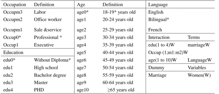
Table 4.1 Variable Descriptions---34
Table 5.1 Descriptive Statistics(Mean)---35
Table 5.2 Occupational Wage Distribution By Quantile---15
Table 5.3 Raw Gender Wage Gap Distributions---16
Table 5.4 Adjusted Gender Wage Gap Distributions In Public Administration--16
Table 5.5 Adjusted Gender wage Gap Distributions In Subsections---17
Table 5.6 Distribution Of Employees Per Quantile(%)---36
Table 5A Mincer Earnings Equations of Public Administration Sector---37
Table 5A1 Interaction Terms In Regressions Of Public Administration Sector--19
Table 5B Oaxaca Decomposition Of Public Administration Sector ---39
Table 5B1 Essential Results Of Unexplained Wage Gap In Public Sector---20
Table 5B2 Value(log points) and Percentage Of Unexplained Wage Gap Of Total Difference in Public Sector---21
Table 5C Mincer Earnings Equations Of Sale & Service Category---41
Table 5C1 Estimated Interaction Terms Of Wage Equation In Sale & Service Category---22
Table 5D Mincer Earnings Equations Of Office Worker Category---42
Table 5D1 Estimated Interaction Terms Of Wage Equation In Office Worker Category---23
Table5E Oaxaca Decomposition Of Earnings Differentials In Sale &Service Section---43
Table 5E1 Contribution Of Each Variable To Unexplained Earnings Differentials In Sale & Service Section ---25
Table 5F Oaxaca Decomposition Of Earnings Differentials In Office Worker Section ---45
Table 5F1 Contribution Of Each Variable To Unexplained Earnings Differentials In Office Worder Section ---26
Table 5G Value(log points) and Percentage Of Unexplained Wage Gap Of Total Difference In Subsections---26
LIST OF FIGURES
Figure 5.0 Gender Log Salary Per Occupation ---13Figure 5.1 Distribution Of Occupations Per Gender and Percentage Of Genders Per Occupation---14
Figure. 5.2 Kernel Density Estimates Of Wage Distributions---15
Figure 6.0 Unexplained Portion Of The Total Difference---28
Chapter 1 Introduction
Since the 1950s, gender equality has been considered as a social and economic goal in most countries as gender equality means utilization of the full potential of individuals. The right to equal pay for work is a fundamental right of Quebec women workers since the adoption of the Quebec Charter of Rights and Freedoms in 1976. However Gunderson (1998) using data from the 1990 government of Canada Census found that variations in earnings between male and female workers are still
substantial.
Some studies on wage differentials in Canada have focused on the public and private sectors. Empirical evidence on the public sector pay gap suggests, even after controlling for observable characteristics, a positive wage differential for public sector workers and higher prime for women as compared to men; likewise pay dispersion is usually found to be lower in the public sector with respect to the private sector. Using Labor Market Survey data from 1997, Gunderson et al. (2000) estimate that public sector workers earn a premium of about 9 percent.
In this paper, we investigate gender wage gaps in public sector by comparing different unexplained and explained portions of total difference, using decomposition results from the entire Public Administration sector sample and two subsections (Sale &Service and Office Worker) as well. Most of the empirical studies from which the evidence on discrimination was derived using Oaxaca decomposition, because it provides a quantitative assessment of the sources between male and female wage differentials. We show that the gender wage differential is sensitive to the choice of quantile and that the pattern of premium varies with both genders and skills. We argue that the decomposition of predicted wage gaps at diverse quantiles provides a more accurate set of measures for the size of the part of the wage gap that is attributed to different returns to skills between genders.
Our findings contribute to the existing literature in several ways. To the best of our knowledge, no study of Quebec addresses the issue of gender wage
differentials in public sector. We focus our study in Quebec ,because even Ontario has the largest part of public sector employees(more than 30 percent) compared to Quebec (25 percent),92 percent of Francophone(unilingual)workers of this sector work in Quebec. Except being the only Canadian province that has a mainly French speaking population and French as the essential official language, Quebec distinguishes itself from other provinces in appearance such as culture ,law ,administrative structure, tax and pay systems. If the returns to human capital is higher in public sector respect to the private sector in Canada ( Moore and Newman and Choudhury,1994) and at the same time Richard E. Mueller(1997) found that females are much better off in the public sector as compared to the private sector than males, this study examines if public sector is a fair employer as if work in public sector is the best choice for women, meaning no gender discrimination in this sector. Specifically our study tries to:
*Measure and decompose the gender wage differentials into explained and
unexplained parts separately concerning to the entire public sector and to its subsections(Sale &Service and Office Worker) in Quebec,
and
*Compare the different portions of unexplained wage difference by quantile in public sectors and identify the possible discrimination phenomenon(glass ceiling and(or) sticky floor).
Firstly we use the Mincer’s earnings function to identify effects of education, age, language and occupation effects on earnings. Here we use OLS regressions and unconditional quantile regressions. Then results obtained in the first step are used to decompose the earnings wage gap into explained (result of gender difference in observed covariates)and unexplained (effects of unobserved factors and/or discrimination) parts using the Oaxaca decomposition technique. These first two steps have been repeated for the entire sector and for two subsections.
Our results show that when the wage differential by quantile is decomposed, generally a significant portion is unexplained by observed characteristics (nearly 70 percent for the whole sector and over 80 percent for two subsections) and is mostly
decreasing over the wage distribution. This part due to returns to characteristics becomes lower at the highest quantiles, suggesting that differences in unobserved characteristics are more important at the bottom of the wage distributions where appears the evidence of sticky floor effects.
This paper is divided into six chapters. The next chapter presents reviews previous research in this area. Next in the third chapter, the methodology is outlined and the data are described in Chapter 4.Chapter 5 provides empirical estimates of the human capital factors and their effects on the gender wage differentials are later decomposed into explained and unexplained parts. Conclusions ,some shortcomings of this paper and several suggestions for future studies are presented in Chapter 6.
Chapter 2 Literature Review
For a long time the valuing of men is different from women. Besides even in the developed countries where women have made lots of economic and occupational improvement during the last century, their work continues to be undervalued (Blau & Kahn, 2000).An empirical investigation from Melissa J. Williams Elizabeth and Levy Paluck and Julie Spencer-Rodgers (2010) including four studies about estimation and determination salaries for men and women, presents some understandings for why men earn more than women ,known as the salary estimation effect .Their study show that besides the contribution of conscious consideration of national wage gap ,this phenomenon indicates a male-wealth stereotype , a belief that men should earn more than women .
Since the 1950s, gender equality has been accepted as a social and economic goal in developed countries. Over the last decades, significant progress has been made, but gender wage inequality still exists in most countries. The average gender wage gap is generally smaller in public sector (Gunderson, 1989; Gregory & Borland, 1999;Arulampalam et al., 2007).By analyzing the source of the gender wage gap in public and private sectors wage distributions in Australia ,Juan D. Baron shows that, gender differences in productivity characteristics fully explains the gender wage gap among low-paid workers . However among high wage workers, from 50 to 60 percent of the wage gap faced by women is unexplained by related characteristics .According to their results, education level and demographic characteristics could explain the gender wage gap between men and women in private and in public sector.
Public sector employment attracts workers who are risk-averse (Pfeifer, 2008) and the wage setting occurs in a political environment. Paul W. Mille(2008) examine gender wage gaps in the US by using the data from the 2000 US Census pooled across males and females across a decomposition based on separate regressions for males and females .His results show that male low-wage earners benefit a greater advantage from government sector over their female counterparts than the case of male
high-wage earners ,in other words, sticky floor effect in the female–male pay differential exist in the government sector .This phenomenon is probably due to the difference of pay-setting for male and female public sector workers. Public sector pay gap estimates proved, in general, rather sensitive to sample choice, empirical specification and the group of worker selected (Gregory and Borland, 1999),previous Studies,(INSEE, 1996; Fournier, 2001;Fougere and Pouget, 2004) these studies suggest that in the public sector there is a positive (negative) premium for low (high) skilled workers, and that being a female also grants a positive premium.
The theory of occupational crowding supposes that women choose positions that are socially feminine. They have an inclination to concentrate in low paying jobs and men work more in high paying sectors. Employers often keep better positions for men, discourage women work in without women occupations. Therefore the supply of women is abundant in some fields which prohibits them from requiring equal salary.
Furthermore women are always undervalued in the labor market. Donald E. Lewis (1996) in an early study decomposes the pay gap between men and women by proposing several indices of occupational crowding indices and estimating their values for Australian women and men from 1891 to 1991. He used Data from the Census of the Common wealth (ABS, I89 1 - I99 I) and the Occupational Survey of the Common wealth of Australia to show that women are crowded into a small range of occupations. Even women are becoming less crowded .The decline is less than that for men. 8.8 I per cent female employees are employed as Sales Assistants. As a consequence, refer to men, the overcrowding of women is increasing. In a related study, using data from the survey of Median Weekly Earnings of Full-Time Wage and Salary Workers by Selected Occupations Requiring Emotional Labor (2000),Mary Ellen Guy (2004) shows the tendency for men and women to work in different occupations(job segregation) ,this conclusion is often considered as one important reason of gender wage gap. The traditional job pay scales often exclude compensation for emotional labors. It was argued that this arises because the emotive work (caring, negotiating, empathizing, smoothing troubled relationships, and working behind the scenes to enable cooperation) is thought to be natural for Women (England and Folbre 1999) and a majority of this part of work is invisible, as a result it's uncompensated, without being contained in job descriptions or evaluations.
There are few studies that examine intra-sector segregation and fewer that test with econometric models of hierarchical discrimination. The model of hierarchical
segregation in Bald-win, Butler, and Johnson (2001) is used for measuring the existing of endowments, pure wage discrimination, and job segregation by DINA Shatnawi And Ronald Oaxaca (2012).They use data from a supermarket and also by using CPS data for purpose of generalization to prove that a misspecification of wage structure might cause incorrect evaluation of pure wage discrimination.
From previous studies ,it's evident that most of women stay in lower-echelon occupations for cultural and human capital reasons. There are multiple barriers in theirs career promotion. Yekaterina Chzhen and Karen Mumford (2010) use quantile regression decomposition based on Machado and Mata (2005) to analyze the gender log wage gap across the distributions of full time workers in British with sample
selection adjustments. The study has found existence of glass ceiling effect in the data and a positive selection of women into full-time work.
It has been shown that the glass ceiling doesn't exist only at horizon level but vertical at the same time. Giovanni Russo and Wolter Hassink(2012) explore the consistent evidence of both vertical and horizontal glass ceiling effect (between and within job levels) in wage growth for women by using an employer–employee matched data set from administrative records of a broad sample of firms from all economic sectors which was constructed by the Dutch Ministry of Social Affairs and Employment(Venema and Faas1999).They document that half of the unexplained gender wage gap is due to multiple glass ceilings faced by women .However the margin effect of horizontal glass ceiling isn't clearly quantified.
Chapter 3 Methodology
In this paper, we assume that the linear quantile regression model is correctly specified. Little is known in the case of misspecification. Angrist, Chernozhukov and Fernandez-Val (2005) give first results on this subject. The OLS regression provides consistent estimate of marginal effect of an explanatory variable on the population unconditional mean of the dependent variable. Because the conditional mean due to the law of iterated expectations averages up to the unconditional mean. As a result, OLS estimates of the dependent variable indicate what is the impact of a covariate on the population average of the explained variable .
Most studies have adopted the human capital model proposed by Mincer(1958)as the theoretical base for the hourly earnings function. It is assumed that wages increase with accumulated skills such as education at the individual employee level. Education is measured by the highest level attained for each individual in this paper.
Furthermore other human capital factors such as age; occupation; language ability; and matrimonial status effect the variation of earnings function.Consequently, I estimate the log of hourly wage as follow:
Yi=Xi’β+ui (3.1)
Where Y presents log hourly wage ,X contains a set of human capital factors chosen from dataset and their interaction terms with the variable Women, including age; education; language ability and occupations. Due to similar characteristics, some variables of occupation are united together. More details are indicated in Chapter 4 and variable definitions is provided in Table4.1(Appendix).The subscript ‘i’ implies various observations, it takes the value of a whole number range from 1 to 3553 for our study in the sector of Public Administration in Quebec. We also proceeded heterogeneity tests for using robust regressions(Table 3.0 Appendix).
In general ,given perfect multicollinearity ,which manifests by a perfect linear relationship between two independent variables in the same regression, it is
technically impossible to calculate estimators. For this reason, I omit variables such as age0(individual aged between 18 and 19 ) ;education 0 (person who has less than high school as highest level attained ) ;occupation0(professional) ;bilingual. Hence the basic group in the regression of the log of hourly wage is a male aged from 18 to 19
years old who worked as a professional in the sector of Public Administration and has not completed high school education and speaking both French and English. In addition, when we study the margin effect of an independent variable contributes to the estimation of the dependent variable, irregular results can be caused by
multicollinearity. This problem arises in a multiple regression when several independent variables are strongly correlated.
Therefore the variable of number of child isn’t included in regression due to correlation with age of woman.1And more specifically, coefficients of these variables of child are barely significant. When it concerns other aspects of the distribution of regressand, other methods have to be used. A way of characterizing the distribution of Y is to compute its quantiles by conditional quantile regressions. However,
conditional quantiles do not average up to their unconditional population counterparts and can’t estimate the impact of X on the corresponding unconditional quantile. To solve this problem, we first have to obtain the estimated recentered influence
functions, and using an unconditional quantile regression proposed by Firpo, Fortin, and Lemieux.Plantenga and Remery (2006) examine the unconditional gender wage gap for 24 EU states (except Malta) plus Iceland. Then we can divide the wage structure and composition effects into the contribution of each covariate, just as in the usual Oaxaca-Blinder decomposition.The recentered influence function is defined as:
RIFji=q(j)+[1(Yi≥q(j)-(1-j)]/f(q(j)] (3.2)
Where q(j) is the jth quantile ,1(.) is a dummy variable equals to 1 if Y is superior or equal to q(j) for individual i,or 0 otherwise f(q(j)) is the jth quantile salary density. Then we have to replace Y by RIF and process a regression similar to OLS.
The procedure known as the Blinder-Oaxaca decomposition (Blinder 1973; Oaxaca 1973) is used frequently to decompose mean differences in log wages of two groups in labor market based on regression models with counterfactual method. The wage differential is always divided into two parts, one is “explained” by differences characteristics observed such as education or work experience ,another part is unobserved nominated as “unexplained” .Discrimination could be contained in this unexplained part, however it could be occurred due to other factors unobserved as well.
Concretely in this paper, the sample is subdivided into one group for women (F) and another for men (M),given a dependent variable as log of hourly wage(Y) , (X) as a serie of predictors including several human capital factors :age; education, language ability, matrimonial status and occupations. From the linear model, we have:
Y=Xι’βι+єι,E(єι)=0,ι∈ {F,M} (3.3) E(Yι)=E(Xι’βι)=E(Xι)’βι (3.4)
D=E(YM)-E(YF)=E(XM)’βM -E(XF)’βF (3.5)
Where D is the mean difference of salary between women and men.After the estimation of βι, according to Oaxaca technique the difference D can be written as:
1 ‘In 2005, women between 30 and 34 years of age became those with the greatest propensity to give birth, followed very closely by women aged 25 to 29. Women aged 25 to 29 had been the most fertile since the late 1960s.’-Statistics Canada
[E(XM)’-E(XF)’]βM+E(XF)’(βM -βF) (3.6)
The first part as explained by different labor force characteristics and the second as unexplained determinant factors of log of hourly wage. I chose the 10th ; 50th ; and 90th quantiles for decomposition as mentioned by Boudarbat & Lemieux (2010),these quantiles are sufficient for gender wage gap study.
Chapter 4 Data and Variables
The observations used in this analysis were taken from the 2006 Census of population Canada which is a nationally representative sample of private Canadian households every five years .All members of these households aged 16 or over were interviewed. The sample size for 2006 is 844,476. In order to focus on those who work in Public Administration (based on the North American Industry Classification System (NAICS) 2002, Canada.),I restrict the sample to individuals who are Canadian citizen by birth ,not belong to a visible minority or aboriginal peoples in Canada as defined by the Employment Equity Act .
Among Australian studies with respect to the part-time and full-time wage gap , Preston (2003) found a significant penalty equal to 8.9 per cent (in 1990) whereas in the Austen et al(2008) study using 2006 HILDA data no significant difference was found in the earnings of full-timers and part-timers. To get around the possible inaccuracy cause by this factor to analysis of gender wage gap in Public
Administration ,in terms of full-time wage data, I deleted observations lacking a reported wage and who did not work full-time or nonresponses.
In the wage equations, the dependent variable is the natural log of the hourly wage. The hourly wage is calculated as earnings during the year 2005 divided by annual working hours ,which is from the multiplication of numbers of working weeks and working hours per week, these two variables are provided in census. In Canada , each province and territory has its own minimum wage. The lowest general minimum is that of Alberta (CA$9.75 per hour) and the highest is that of Nunavut (CA$11.00 per hour) in 2012.Until 2011 The Employment Standards Act of British Columbia allowed employers to pay as little as CA$6 per hour to new workers with less than 500 hours of work experience .As a result individuals who have wages below 7.6 dollars or exceeding 150 per hour are not included in the dataset for our study in Quebec. Considering different wage systems among occupations, I include five dummy variables of occupation signalize status of employment :Executive; Office Worker; Professional; Sale & service and Laborer. Some jobs titles from data base are grouped together due to similar occupational characteristics.
A recent study by the US Census Bureau for the US confirms the connection between a person’s level of education and his or her employability and earnings. The study shows that US college graduates earned far more over their lifetimes than people who only graduated from high school. We might see this same connection in the Public Administration sector. The explanatory variables assumed to influence wages include: age; education; language ability ;matrimonial status and occupation. A dummy variable indicating sex of individual was included in regression. Independent
variables such as education ,occupation and age are measured by using dummy variables for different levels(Talbe4. 1). Since Canada is an official bilingual country, maybe someone who can use a second official language get paid more. Thus three dummy variables are designed: Bilingual, English, French. Individuals without English nor French understandings are dropped out due to low frequency in Public Administration . In addition, all individuals have lacking data for variable of interest were deleted from the dataset. This leaves a sample of 1,928 males and 1,625 females in Quebec(total 3553 individuals).
Chapter 5 Results
This chapter presents some descriptive statistics following by the empirical results on earnings and earning gaps, obtained using the techniques and data sets described in chapter3.Firstly the results are concluded from regression of overall Public Administration sector and thereafter in the 10th ;50th;90th quantiles of adjusted wage distribution(RIF). These are followed by results derived from decomposition of earnings gaps into explained and unexplained gaps within this public sector. Then the same procedure is applied to two subsections namely: Sale &Services and Office Worker.
5.1 Descriptive Statistics
In terms of the explanatory variables that we used to explain variation in log of gross hourly wages, there are some important differences between genders. It is
assumed that wages increase with measures of accumulated human capital factors such as education and work
experience. In Table 5.1(Appendix), we give some descriptive statistics for the key
variables computed on the subsample of the Public Administration workers and
disaggregated by gender and occupational indicators. As expected, taking into account all workers, we can say that men’s wages are on average higher than women’s wages for each occupation(Figure 5.0).The results indicate that on average as Executive employees they earn higher wages than the other four sectors’ employees. The gender wage gaps, measured by the difference in log wages between men and women, is about 17% for Executives, 11% for
professionals, 21 % for Sale &Service and about 20 percent for office workers. This effect is lessen if we consider the position for labor workers where the gap is 9%.It should be noted that for labor workers the gender gap is lower despite the fact that the average hourly wages for them are lower relative to the other occupations.
Looking at the unconditional differences can be misleading if the endowments of the groups are different. Hence, we will investigate how individual characteristics, such as educational attainment, marital status vary across workers within these five
occupations. In fact, there are not notable differences on average in the characteristics of employees through type of employment. Among those working in Public
Administration and reporting wages, men are on average older than women for each type of occupation, and levels of education are slightly higher for men than for women. Lowest paid (labor force in this paper)men working full-time are on average 42.5 years old compared to 40 years old for women ,where occurs the largest age gap, nearly 2 and a half years between genders. In sum ,wage increases with age, however the exception exists for individuals in sector of Sale &Service who earn more than Laborer and Office Workers but have the lowest average age of 38 years old. Finally there is no evidence for positive nor negative correlation between gender age gap inside a profession and average wage raising across different occupations.
Generally, highly educated (over bachelor degree) men earn on average more compared both to highly educated women and to low educated of both genders especially women. Low educated women (between high school and bachelor degree)earn the lowest gross hourly wages (3.02 point of log of gross hourly wage).However we observe that on average for male office workers who earn less than men working in Sale &Service, their mean value of education indicator is 0.18 points higher. This is not the case for women.
Recent work from the sociology literature also supports the finding of gender differences in occupational employment. Thus, Figure 5.1we plot the distribution of occupations per gender across the hierarchical job ladder. It indicates that more than 80 percent of women are concentrated in two rungs of occupation: Office Worker(52 percent) and Professional(33 percent).Meanwhile the most popular occupations for men are professional and in the sector of Sale &Service which represents nearly 30 percent each. At the same time the percentage of women per occupation presented in Figure 5.1 indicates that female employees represent 76% of total employment in the sector of Office Worker. In contrast, for entire labor employees ,just 8 percent
employees are women.
Figure 5.1 Distributions Of Occupations Per Gender and Percentage Of Genders Per Occupation
The elderly and high paid employees are considerably more likely to be married .On average 53.66% of women is married at age of 43.5 in contrast to 39.39% at age of 37.5.In each occupation ,the percentage of married men workers is higher than married women, especially for low educated and low paid jobs (49.41% of labor male
workers is married against 33.33% of labor female workers). With the same average age (40 years old),nearly half of the female professional workers are married and just one third of women who worked as labor.
French is the second language that most employers in Canada look for outside Quebec, the demand for people who can work comfortably with multiple languages is rising fast, particularly in areas such as tourism where lots of interactions with people are presented. However except the public service ,most Canadian jobs don’t require bilingual fluency.97% of all individuals who speak only French in public sector work in Quebec. Meanwhile there is no English speaking person working as labor in the Public Administration for both genders without French ability and for female workers in occupation of Sale &Service(but two male employees out of 651 workers in this category).The opposite has been happening as regards French ,almost 68% of male labors and 50% of female working in Sale &Service only speak French. Additionally, among those who are bilingual, the proportion increases markedly with job ladders. The majority (70.90% of male and 58.54% of female) of Executives manage both language compared to 32.02 % of men working as labor and 47.62 % of female Office Workers. All together men are more bilingual than women across occupations ,gender gap is as much as 19.2% for Office Workers. Nonetheless, the position is changed concerning about labors workers. Upwards of 48% of female compared to 32.02% of male can speak a second language.
For each occupation, we have determined the wage distribution. Remarkably, there is a substantial overlap in wage distribution between adjacent hierarchical occupational jobs (see Table5.3). The first decile of the wage distribution at a specific occupation k (k = 1,…,5) is always below the third decile of the wage distribution of the level directly below (level k-1). To quantify the degree of overlap, the seventh line in Table 5.2 shows the percentage of workers at job level k whose wage is below the third decile of the wage distribution at job level k-1.The degree of overlap does not differ substantially among all workers. This brings us to the important conclusion that information on the overall wage distribution per se is not sufficient to investigate gender segmentation at different occupation levels .
Table 5.2 Occupational Wage Distribution By quantile
Quantiles 5-Executive 4-professional 3-Service 2-officeworker 1-laborer
10 2.6591935 2.662752 2.430482 2.450738 2.5045 30 3.2992435 3.162014 3.027384 2.928834 2.8962 50 3.562431 3.346498 3.256672 3.0861755 3.06304 70 3.693718 3.5228185 3.4426815 3.255357 3.21233 90 3.9629805 3.732917 3.7311875 3.483729 3.36111 Overlap% 0.8409809 0.879555418 0.82984628 0.8461723
Table 5.3 shows that the overall wage distribution increasing gender wage gap pattern: the raw gender wage gaps are generally increasing across much of the support of the wage distribution but then decrease as we move into the upper tail of the wage
distribution. Subsequently we consider the development of the gender wage gap at each occupational level to investigate whether it is consistent with the presence of an intra-level increasing or decreasing pattern.
The raw gender wage gap at each occupational level, not yet corrected for workers’ observable characteristics, is shown in Table5.3. The wage gap across the deciles of the intra occupational level wage distributions displays an intricate pattern: There is no clear relationship between the size of the gender wage gap and the centiles for laborer and professional categories. Contrary to these two jobs before, table 5.3 shows evidence of gap reducing in Sale &Service and Executive job levels. The strongest evidence of decline is found in the category of Executive. Finally, the presence of an booming salary difference in intra-occupation level existed just for office workers. The negative sign of wage gap at the 90th quantile in section Executive and at the 10th quantiles for Office Workers ,exhibits an advantage of female employees towards their male colleges.
Interestingly we can see a positive correlation between the percentage of women within a specific occupation and the width of gender wage gap in the upper tail of the wage distribution, the greatest salary difference is presented in Office Worker at the 90th quantile where exist the largest percentage of female employees among all occupations.
Table 5.3 Raw gender wage gap distributions
Quantiles Executive Professional Sale &Service Office Worker Laborer Overall 10 0.585833 0.175136 0.470872 -0.011349 0.003752 0.191315 30 0.267951 0.106884 0.33706 0.18157 0.127966 0.225343 50 0.132588 0.133166 0.313024 0.216913 0.068417 0.246842 70 0.11071 0.106443 0.266931 0.24864 0.020845 0.265807 90 -0.06050 0.077692 0.077993 0.344277 0.084812 0.169925 %women 34 45 20 76 8 100
With correction for workers’ observable characteristics by running a regression of recentered influence function (RIF) ,firstly we find the same plan for the entire sector (Table 5.4):a growing wage difference appears with higher quantile, however at the 90th quantile ,this difference declines to the lowest level. And this deviation increases from 0.021 anteriorly without control of human capital factors to 0.069 after.
Table 5.4 :Adjusted Gender Wage Gap Distributions In Public Administration
Overall Quantile10th Quantile50th Quantile90th
Women 3.174 2.710 3.148 3.701
Men 3.388 2.907 3.399 3.836
Difference -0.214 -0.197 -0.251 -0.136
The descriptive statistics presented in Table 5.4 after correction reveals that the gender wage gap is not uniform throughout the wage distribution in these two
categories ,nevertheless both of them remain the same trend .We can note that , at the top of the wage distribution, the gender wage differential in office workers’ section is similar to that at the bottom of the wage distribution for sale & service workers. The volumes of difference between the 10th and the 90th quantile become smaller for office and larger for sale &service employees.
Table 5.5 :Adjusted Gender wage Gap Distributions In Subsections
Sale &Service
Overall Quantile 10th Quantile 50th Quantile 90th Women 3.159 2.525 3.163 3.767 Men 3.409 2.912 3.462 3.832 Difference -0.251 -0.387 -0.299 -0.064 Office Worker
Overall Quantile 10th Quantile 50th Quantile 90th Women 3.027 2.669 3.014 3.391 Men 3.252 2.813 3.229 3.739 Difference -0.225 -0.145 -0.216 -0.347 Note: Difference=Women-Men
The mean log wage gap may, however, hide important differences across the wage distribution, such as those between low earners and high earners. The distribution of earnings is considered in greater detail in Fig.5.2 which plots the densities estimated using an Epanechnikov kernel estimator of wages for men and women working full-time in Public Administration and by different occupations. The distribution of male wages of the whole public sector is essentially symmetric, while the corresponding female distribution is rather skewed to the left.
It can be seen from these figures that the distributions are quite distinct between occupations and especially for women. The office workers’ and professionals’ earnings distributions are characterized by a higher density function around the mode and a lower dispersion for both genders. For females, the Executive section earnings distribution lies within the male’s distribution function around the peak area.
Figure. 5.2 Kernel density estimates of wage distributions
There should have enough employees both in the upper and lower tail to apply unconditional quantile regression which is the case of our data set for the whole sector and for the two chosen sections :Sale &Service and office workers. More details for distribution of employees by quantile were in Table 5.6 of appendix.
5.2 Public Administration Sector Regressions Results
In Public Administration the mean log hourly wage for males was 3.38 log points (CA$30/h) and the corresponding female mean wage was 3.17 log points (CA$24/h).Thus the resulting log wage differential was 0.21 points, and the mean wage difference was CA$6/h.
The Blinder-Oaxaca decomposition for these differentials using equation (3.6) ,it is estimated that on average approximately 70% of the log wage difference was due to skill or productivity advantage evaluated as it would have been in the absence of discrimination. Translated into dollars and cents it means that about 0.8 of the 1.23 log points wage gap was due to skill differences between men and women. The male treatment advantage accounted for a large part of the log wage differential and about 24% of the mean male wage .
5.2 A Mincer Earnings Equations of Public Administration
The human capital covariates could have different effects on salary. Hence, Table 5A (Appendix) provides results from ordinary least squares (OLS) estimation of the determinants of wages for all full-time employees in Public Administration and results by quantile.
Unsurprisingly, staff members are found to be significantly likely to make more money if they are older (accurately assumed to have more years of work experience) ,especially at the lower tail. The estimated parameters inform us about the age covariate impact on wage. Only for workers locate in the 10th quantile of wage distribution ,nearly all age covariates positively and significantly affect wages.The value of each coefficient in this quantile is relatively large. For a person in the age range of 35 to 39, the estimated prime is as important as 1.31 log points.Wages increase at a increasing rate from 20 up to 39 years old then at a diminishing rate through the accumulation of experience. In the 90th quantile, the position is quite different. Age affect negatively the salary except for employees above 64 years old.
However estimated coefficients are statistically significant just for individuals aging from 30 to 34(-0.55 log points ) and from 20 to 24(-0.54 log points).
If we take derivative of age, we could find that in Public Administration , males in the 45-49 age group and females in the 40-44 age group have the highest average wages:3.44 log points for men and 3.23 log points for women. The standard deviation of mean for 18–19 age group (reference group)is roughly higher than that for employees between age 20 and 24 even the estimated coefficient is 0.25 log points higher.
Women aging from 20 to 24 earn 0.45 log points higher than men in their age group in the 50th quantile. Observations from our dataset point to the fact that the standard deviation of mean salary for men is superior to that of women although their mean salary is slightly higher (0.05 log points).The rest of interaction terms of age and female are positive nevertheless they are statistically unsignicifant across all quantiles regressions and the regression of the overall sector(Table 5A1).
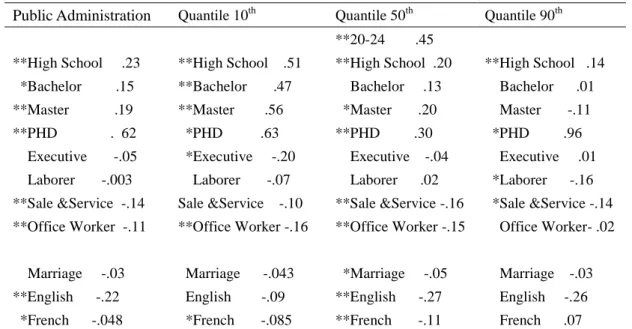
Table 5A1 Interaction Terms In Regressions Of Public Administration Sector Public Administration Quantile 10th Quantile 50th Quantile 90th **High School .23 *Bachelor .15 **Master .19 **PHD . 62 Executive -.05 Laborer -.003 **Sale &Service -.14 **Office Worker -.11 Marriage -.03 **English -.22 *French -.048 **High School .51 **Bachelor .47 **Master .56 *PHD .63 *Executive -.20 Laborer -.07 Sale &Service -.10 **Office Worker -.16 Marriage -.043 English -.09 *French -.085 **20-24 .45 **High School .20 Bachelor .13 *Master .20 **PHD .30 Executive -.04 Laborer .02 **Sale &Service -.16 **Office Worker -.15 *Marriage -.05 **English -.27 **French -.11 **High School .14 Bachelor .01 Master -.11 *PHD .96 Executive .01 *Laborer -.16 *Sale &Service -.14 Office Worker- .02 Marriage -.03 English -.26 French .07 Note: **Statistically Significant Coefficients At 5 Percent Level
*Statistically Significant Coefficients At 10 Percent Level
Being married are significantly more likely to have higher salary, which is around 0.055 log point compared to single workers for men and women. Marital status also generally affects wage in the same way for both genders, besides in the 50th quantile, women suffer from a faintly disadvantage of 0.05 log points of salary .
In contrast, a Francophone without being bilingual and particularly being a female is strongly negatively related to the salary they could earn in this sector, respectively from 0.03( in the 10th quantile) to 0.13 (in the 90th quantile )less log points of salary for all the stuff and add between 0.05 to 0.11 points disadvantage for women.
Higher education in general is associated with higher wages, this effect is obvious in the upper tail and in the whole sample. Undergraduate level yield 0.18 log points of higher paid per hour .A PHD owner could have up to 48 percent advantage
of hourly wage compared to workers without any diploma in the 90th quantile. For high school level education, the coefficient is negative(-0.03)and statistically significant for high paid workers. Most coefficients are statistically significant ,despite the fact that there are gender differences in returns to educational attainment, characterized by important pay advantages of the PHD degree for female employees and especially for women with lower salary. They have at least 0.5 log points for more than male workers with the same level of education in the 10th quantile of wage distribution.
Furthmore, in terms of significance, the impact of occupational categories is rather important.The mean value of log hourly wage increase with career ladders. The highest paying occupation is Executives. On average ,being an Executives in Public Administration raise 14 percentage log points of hourly salary compared to professionals. Manual workers could see a decrease of 22 percent in regard to average wage by being the lowest level of occupation .Working in the sector of Sale &Service could gain 5 percent however within this group of workers, there appears quite substantial differences between genders. Female workers earn 14 percent per hour less than their male colleges. Women working in office are in the same situation with less disadvantages(11 percent).Nevertheless, coefficients of Executive section and Office Worker category decline as moving up from lower to upper quantile. In the 90th quantile, we note that all coefficient of occupations are not significant at 5 percent level and only coefficients of Laborer and Sale &Service categories are still significant at 10 percent level.
5.2 B Explained and Unexplained Gaps of Public Administration
Sector
We use the Oaxaca decomposition technique to decompose the male and female earnings differentials into explained and unexplained portions(Table5B Appendix),the method is described fully in Chapter3.Table 5B1 and Table 5B2 shows the contribution of unexplained factors to overall earnings differentials in the public sector and separately by quantile. Using our results, we can estimate the contribution of each of the variables to the overall differential.
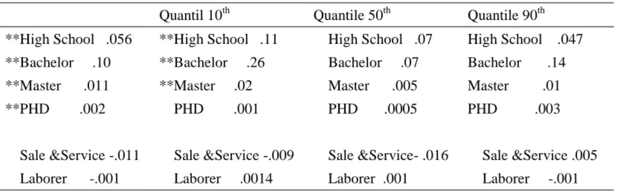
Table 5B1 Essentials Results of Unexplained Wage Gap In Public Sector
Quantil 10th Quantile 50th Quantile 90th **High School .056 **Bachelor .10 **Master .011 **PHD .002 Sale &Service -.011 Laborer -.001 **High School .11 **Bachelor .26 **Master .02 PHD .001 Sale &Service -.009 Laborer .0014 High School .07 Bachelor .07 Master .005 PHD .0005 Sale &Service- .016 Laborer .001 High School .047 Bachelor .14 Master .01 PHD .003 Sale &Service .005 Laborer -.001
**Office Worker-.055 Executive .004 Marriage -.014 *French -.023 **English -.003 Office Worker -.005 **Executive -.014 Marriage -.021 French .002 English -.002 Office Worker -.06 **Executive -.011 Marriage -.014 **French -.04 *English -.003 **Office Worker -.06 **Executive .02 Marriage .0009 French -.02 English -.004
Note: **Statistically Significant Coefficients At 5 Percent Level *Statistically Significant Coefficients At 10 Percent Level
Table 5B2 Percentage Of Unexplained Wage Gap Of Total Difference In Public Sector
Overall Quantile 10th Quantile 50th Qauntile 90th
% 70 85 68 47
Unexplained -0.149 -0.165 -0.169 -0.063
The unexplained portion in the whole public sector is -14.9 percentage points(male employees as reference group). This indicates that nearly 70 percent of the overall gender wage differential is due to unexplained factors. Among different quantiles, this figure varies from 0.17 to 0.06 percentage points by moving up in centiles .Thus the corresponding unexplained part portion change from 85 to 47 percent of the gender wage gap which means that women receive relatively fair-pay in the upper quantile. Where appears evidence of sticky floor phenomenon.
Advantage of educational attainment returns particularly affect the amount of salary of a female employee in this sector. The total value of educational coefficents is 0.17 in unexplained part .Effect of education reduces with larger quantiles. In the highest quantile, these coefficient are not statistically significant at ten percent level. Meanwhile about half of the explained difference was included in educational factors in the 10th quantile.
In the public sector, with respect to the explained gap, the productivity factor “age” can explain 2.0 percentage point of wage disadvantage of females. At the same time a female employee between age 45 and 49 enjoys a benefit of 1.6 percentage point of salary. The wage advantage of males can also be explained by their higher earnings occupational which contribute 4.7 percentage points to the explained portion and their language ability which contributes 12% .A positive entry for laborer category indicates an advantage for females, but this positive number in the explained gap are very small or statistically insignificant concerning age groups. For females, there are no important age factors that have a substantial impact on their wage advantage unless for the lowest quantile concluding 1.2 percentage points by adding up five statistically significant age coefficients.
5.3 Subsections Regressions Results
5.3A Mincer Earnings Equations of Sale &Service and Office Worker
categories
The returns of characteristics estimate of entire sample and at the 10th ;50th and 90th percentiles are reported in Table 5.C of the appendix for Sale &Service subsection. The results for the Office Worker section are reported in Table 5.D (Appendix).These estimates suggest that the wage determination process differs according to gender within each section and remarkably affected by age factors. In fact the log hourly salary grows rapidly with accumulation of this factor.
For employees in Sale &Service section salary increasing with age between 20 and 59.For employees in the 35-54 age group they get nearly 1 points higher log hourly wage than the reference age group(aged 18-19).These coefficients are generally statistically significant except for the 90th quantile in this section. In the Office Worker section, we found the same impact of age on salary :being older provides higher wage besides the highest-paid employees in the age of 20 to 29 or more than 64 years old. Unlike for workers of Sale &Service ,these negative coefficients become statistically significant at 5 percent level.
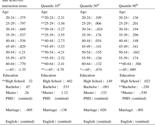
Table 5C1 Estimated Interaction Terms of wage equation in Sale &Service category
Sale &Service
interaction terms Quantile 10th Quantile 50th Quantile 90th Age: 20-24 | -.375 25-29 | -.797 30-34 | -.669 35-39 | -.537 40-44 | -.536 45-49 | -.829 50-54 | -1.21 55-59 | -.675 60-64 | -.770 >=65 | -1.35 Education **High School| .32 Bachelor | .07 Master | .26 PHD | (omitted) Marriage | -.005 English | (omitted) Age: **20-24 | -2.21 **25-29 | -3.56 **30-34 | -3.27 **35-39 | -3.55 **40-44 | -2.73 **45-49 | -3.53 **50-54 | -4.21 **55-59 | -2.32 **60-64 | -2.41 **>=65 | -4.70 Education High School | . 462 Bachelor | .533 *Master | 1.12 PHD (omitted) Marriage| -.138 English | (omitted) Age: 20-24 | .109 25-29 | .006 30-34 | -.024 35-39 | .176 40-44 | .034 45-49 | -.141 50-54 | -.155 55-59 | -.126 60-64 | -.132 *>=65 | -.674 Education High School | .149 Bachelor | -.091 Master | .133 PHD | (omitted) Marriage | .020 English | (omitted) Age: 20-24 | .136 25-29 | .201 30-34 | .194 35-39 | .296 40-44 | .148 45-49 | .341 50-54 | -.042 55-59 | .174 **60-64 | .366 >=65 | .009 Education High School | .022 **Bachelor | -.250 *Master | -.530 PHD | (omitted) Marriage| -.001 English | (omitted)
**French | -.220 French| -.057 **French |-.190 *French | -.147 Note: **Statistically Significant Coefficients At 5 Percent Level
*Statistically Significant Coefficients At 10 Percent Level
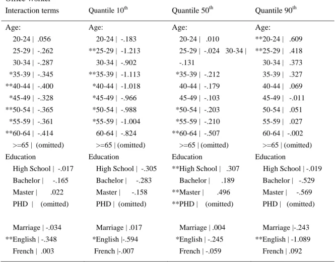
Table 5D1 Estimated Interaction Terms of wage equation in Office Worker category
Office Worker
Interaction terms Quantile 10th Quantile 50th Quantile 90th Age: 20-24 | .056 25-29 | -.262 30-34 | -.287 *35-39 | -.345 **40-44 | -.400 *45-49 | -.328 **50-54 | -.365 *55-59 | -.361 **60-64 | -.414 >=65 | (omitted) Education High School | -.017 Bachelor | -.165 Master | .022 PHD | (omitted) Marriage | -.034 **English | -.348 French | .003 Age: 20-24 | -.183 **25-29 | -1.213 30-34 | -.902 **35-39 | -1.113 *40-44 | -1.018 *45-49 | -.966 *50-54 | -.988 *55-59 | -1.004 60-64 | -.824 >=65 | (omitted) Education High School | -.305 Bachelor | -.283 Master | -.158 PHD | (omitted) Marriage | .017 *English |-.594 French |-.007 Age: 20-24 | .010 25-29 | -.024 30-34 | -.131 *35-39 | -.212 40-44 | -.179 45-49 | -.103 *50-54 | -.203 *55-59 | -.210 **60-64 | -.507 >=65 | (omitted) Education **High School | .307 Bachelor | .189 **Master | .496 **PHD | (omitted) Marriage | .004 *English | -.245 French | -.059 Age: **20-24 | .609 **25-29 | .418 30-34 | .373 35-39 | .327 40-44 | .069 45-49 | -.011 50-54 | .051 55-59 | .027 60-64 | -.002 >=65 | (omitted) Education High School | -.019 Bachelor | -.529 Master | -.569 PHD | (omitted) Marriage |-.243 **English | -1.089 French | .092
Note: **Statistically Significant Coefficients At 5 Percent Level *Statistically Significant Coefficients At 10 Percent Level
Evidence of prejudice is found for women in Sale &Service category concerning age factor(Table 5C1) .The results indicate that women on average earn less than their male colleges across all age groups and these differences increasing with age. The variation is on average between 0.4( in the 20-24 age group )to 1.4 log salary points when they are over 64 years old. .At the 10th quantile where a female worker suffer the most by age factor they could have less 4 log salary points (age 50-54 and over 64 years old).We found the same figure in office worker category (Table 5D1)with smaller coefficient for each age group variable and less portion of coefficients are statistically significant at the 10th quantile .This portion is larger in regression of the entire category.
Higher educated workers commonly earn more salary in both section excluding high school diploma owner working as Sale &Service employee. And within some specific quantiles of Office Worker section we can see the same effect without being statistically significant. For Sale &Service category, they suffer significantly 0.3 points less log salary in the 10th quantile meanwhile at the 90th quantile they have a benefit of 7 percentage points which is significant at 10 percent level. As a result in the regression of this whole section ,the sign of coefficient rest negative but smaller(0.03)and is not statistically significant. Returns to education are very different on average and across quantiles between these two categories for female workers. At lower levels of education, we observe that for office workers, females with a high school degree on average have lower coefficients than males and generally this coefficient is not statistically significant unless at the 50th quantile this coefficient is statistically significantly and positive(0.3 log points).We could notice that this quantile has all educational coefficients with sign positive, in particular for those with a Master diploma as the coefficient is almost 0.5 percentage points.
However, the reverse is observed for high school degree female owners in Sale &Service category. In other words, they actually have higher wage potential than male employees with the same level of education in this section and the coefficient is statistically significant. The largest difference between males and females of a particular educational level is in the 10th quantile for those with a Master degree ,the coefficient of interaction is 1.12 positive log points. Meanwhile there is also a substantial loss of 0.5 log points for female employees at the 90th quantile ,both of them are statistically significant at 10 percent level.
We find that being fluent in English increases hourly wages of Office Workers by 0.2 log points, which is as much as the return to completing bachelor's degree and half of the return to completing a Master’s degree. In the 90th
quantile, the coefficient of English significantly increases 0.84 log points hourly wages. However there is considerable heterogeneity in returns by genders. Females receive lower returns to English across all quantiles and in the whole section regression. These negative effects vary from 0.25 to 1.1 log wage points by quantile where high paid women suffer the most. All interaction terms of female and English are statistically significant for regressions of office section. The premium for English skill whereas appears for worker as Sale &Service employees, it is not statistically significant across all regressions and there is no evidence of gender impact on this factor.
The negative coefficient in earnings functions of French for unilingual individuals is generally larger in the case of Office Worker than in Sale &Service section. Wages are on average 9% lower for staff who speak fluent French but not bilingual and 29% lower at the 90th quantile for office worker. Even though we do find that wages decline for unilingual Francophone at 50th quantile in Sale &Service sub-group by 0.1 percentage points, the returns are not considerably lower at other quantiles or for the whole section on average.
Being married could earn more than singles, our results indicate that on average they have the benefit of 4 to 5 percentage points in both sections ,and wages for married men are more than married women in spite of these coefficients are not
statistically significant.
5.3 B Explained and Unexplained Wage Gaps of Sale &Service and
Office Worker categories
We used the decomposition method proposed by Oaxaca–Blinder to calculate mean wage decompositions by sections and its extension method by quantile within each section. The results are reported in Tables 5E and 5F of appendix for Sale &Service and for office employees respectively.
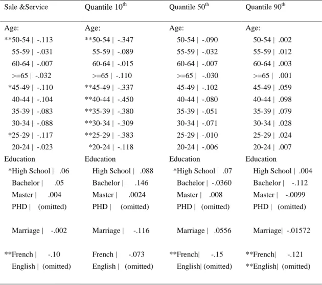
Table 5E1Contribution of each variable to unexplained earnings differentials In Sale &Service Section
Sale &Service Quantile 10th Quantile 50th Quantile 90th Age: **50-54 | -.113 55-59 | -.031 60-64 | -.007 >=65 | -.032 *45-49 | -.110 40-44 | -.104 35-39 | -.083 30-34 | -.088 *25-29 | -.117 20-24 | -.023 Education *High School | .06 Bachelor | .05 Master | .004 PHD | (omitted) Marriage | -.002 **French | -.10 English | (omitted) Age: **50-54 | -.347 55-59 | -.089 60-64 | -.015 >=65 | -.110 **45-49 | -.337 **40-44 | -.450 **35-39 | -.380 **30-34 | -.309 **25-29 | -.383 *20-24 | -.118 Education High School | .088 Bachelor | .146 Master | .0024 PHD | (omitted) Marriage | -.116 French | -.073 English | (omitted) Age: 50-54 | -.090 55-59 | -.032 60-64 | -.007 >=65 | -.030 45-49 | -.102 40-44 | -.080 35-39 | -.051 30-34 | -.071 25-29 | -.010 20-24 | -.006 Education *High School | .07 Bachelor | -.0360 Master | .008 PHD | (omitted) Marriage | .0556 **French| -.15 English| (omitted) Age: 50-54 | .002 55-59 | .012 60-64 | .003 >=65 | .001 45-49 | .059 40-44 | .098 35-39 | .079 30-34 | .028 25-29 | .024 20-24 | .007 Education High School | .004 Bachelor | -.112 Master | -.0099 PHD | (omitted) Marriage| -.01572 **French| -.121 **English| (omitted) Note: **Statistically Significant Coefficients At 5 Percent Level
*Statistically Significant Coefficients At 10 Percent Level
Table 5F1 Contribution of each variable to unexplained earnings differentials In Office Worker Section
Office Worker Quantile 10TH Quantile 50th Quantile 90th Age: 50-54 | -.0763033 55-59 | -.0304531 60-64 | -.0050556 >=65 | (omitted) 45-49 | -.0937443 40-44 | -.0704109 35-39 | -.0371051 30-34 | -.0175054 25-29 | -.0089636 20-24 | .0015776 Education: High School | -.006 Bachelor | -.103 Master | .0001 PHD | (omitted) Marriage | -.016381 French |.0017447 English | -.003401 Age: **50-54 | -.277986 **55-59 | -.1182553 60-64 | -.013 >=65 | (omitted) **45-49 | -.3575473 **40-44 | -.2406206 **35-39 | -.1351262 *30-34 | -.070 **25-29 | -.050 20-24 | .00056 Education: High School -.103 Bachelor | -.227 Master | -.002 PHD | (omitted) Marriage | .0297 French | .0600 English | -.0034 Age: 50-54 | .005844 55-59 | .006647 60-64 | -.000252 >=65 | (omitted) 45-49 | .006373 40-44 | -.001746 35-39 | -.01404 30-34 | .005454 25-29 | .008859 20-24 | .005225 Education: High School | -.011 Bachelor | -.104 Master | .0005 PHD | (omitted) Marriage|-.0201286 French| .0068088 English| -.0030277 Age: 50-54 | .045 55-59 | .026 60-64 | .0018 >=65 | (omitted) 45-49 | .041 40-44 | .043 35-39 | .045 30-34 | .015 25-29 | .007 20-24 | .006 Education: High School| .048 Bachelor | .014 Master | .003 PHD | (omitted) *Marriage | -.072 French| -.040 **English| -.009 Note: ** Statistically Significant Coefficients At 5 Percent Level
*Statistically Significant Coefficients At 10 Percent Level
Table 5G Value(log points) and Percentage Of Unexplained Wage Gap Of Total Difference In Subsections
Office Worker
Overall Quantile 10th Quantile 50th Quantile 90th
Unexplained -0.181 -0.159 -0.185 -0.267
% 81 94 88 77
Sale &Service
Overall Quantile 10th Quantile 50th Quantile 90th
Unexplained -0.215 -0.327 -0.264 -0.043
% 86 83 88 74
In Office Worker section, the unexplained portion (Table5.G)accounts for 18.5 percentage points (88 percent) of the total wage differential. And within individual quantile, this figure is quite the same, particularly reaching 13.3 percentage points (94
percent) for the lowest and 26.4percentage points (77 percent) for the highest quantile. Hence in the 10th quantile, the gender wage gap is not explained by human capital variables but rather by other covariates or discrimination factors. Age negatively affect wage for low paid female workers, they suffer a total disadvantage of 1.25 log salary points especially for the 45-49 age group(Table 5F.1).Individually ,on average the estimated gender wage gap due to differences in the returns to characteristics is not statistically significant for employees in this section. For those who belong to the bottom of the wage distribution ,most of the age group coefficients are negative and statistically significant. At the same time the difference in term of return growing with age and varies from 0.05 (between 25-29 years old ) to 0.35 (between 45-49 years old)log points. In addition, the sign of unexplained part of age factors is the same as we have found for interaction terms in OLS regressions. Although for most of the educational factors except in the highest quantiles, their signs are in reverse.
Finally, almost 20 percent of the pay gap is attributable to the uneven distribution of characteristics of human capital among men and women in the Office Worker division. Specifically, men are much more likely to have a Master diploma than women which contributes to two percentage points(67%)of total explained gender salary difference. From 45-49 years of age women has an advantage, the coefficients for this category is approximately 9 percentage points higher than for males, which is larger than total explained part in absolute terms. Summing up the relative statistically significant contributions of the three characteristic controls in decomposition based on mean(age, education and French) suggests that about ten percent of the gap is attributable to an uneven distribution of explanatory variables across the genders(Table 5F in Appendix).
At the 10th quantile, the explained part of difference has sign positive which means
that at the lower tail of wage distribution women should pay more than men based on their human capital factors. The coefficient for individuals in the age range of 45 to 49 is 0.26 and decreases by moving up the wage distribution and becomes statistically insignificant. The educational factor of Master degree influences wage difference at 50th quantile almost in the same way of decomposition based on average .Disadvantage of just speaking French explain on average 45 percent of wage gap and stays significant for median and upper quantiles.
Our results show that the decomposition results based on quantiles and on average statistically say little about explained part of gender pay differences in Sale &Service category of Public Administration .For total explained wage difference ,there is a declining figure across the different quantiles. From about age 45 to 54 ,returns to age for women provides part of the unexplained raison in this sector:on average they have less salary(10.9 percentage points log salary for the 45-49 age group and 11 percentage points for the 50-54 age group) than men at the same age. Female workers between 25 and 29 are in the same position with minus 0.11 log salary points at mean decomposition. At the lower quantile ,age factors have largest impact on gender wage gap .Most of them are statistically significant and negative. The influence reduce at median quantile and return to experience become more beneficial for women at the 90th quantile, however they are not statistically significant. Typically, there is also
more gain for women going from without any degree to have a diploma compared to male employees, of which has the coefficient 0.06 on average and 0.07 in the median decomposition for high school graduate. Other educational coefficients are nearly all positive leaving out the Bachelor and Master level in the upper quantile.
Chapter 6 Conclusions
This paper uses data from the Canada Census Individual Micro data Files of 2006 to estimate earnings functions for males and females in the Public Administration sector and two specific occupations (Sale & Service and Office Worker). Using the Mincer earnings regressions’ results firstly, the gender wage differentials were decomposed into an explained portion and an unexplained portion by usingthe Oaxaca-Blinder (OB) decomposition .Secondly the linear least squares results were further desegregated by quantile using an extension of OB decomposition after replacing the explained variable by estimated recentered influence functions (RIF) and using an unconditional quantile regression (UQR)proposed by Firpo, Fortin, and Lemieux. This decomposition allowed us to study the two above portions in more detail in regards to wage distributions.
We find that the adjusted public sector pay gap with correction for workers’ observable characteristics by running UQR has the same pattern as in the case of raw gender wage gaps, however the deviation between the 10th and the 90th quantile increases after rectification .To the contrary ,this variation has a slight decline in the two subsections (Sale &Service and Office Workers). The upper quantile of gender wage differentials in office workers’ section equals to lower quantile of wage gaps for Sale & Service workers and has a larger disparity.
The unexplained portion (Figure 6)falls generally comparing upper to lower quantiles. For example, 85 percent of the wage gap is attributable to the unexplained part on average in Public Administration in the 10th quantile, while in the 90th quantile this figure is 47 percent. In the Sale &Service