Do we miss the hot spots? ? The use of very high resolution aerial photographs to quantify carbon fluxes in peatlands

(1)

HAL Id: hal-00297982

https://hal.archives-ouvertes.fr/hal-00297982

Submitted on 6 Mar 2008

HAL is a multi-disciplinary open access

archive for the deposit and dissemination of sci-entific research documents, whether they are pub-lished or not. The documents may come from teaching and research institutions in France or abroad, or from public or private research centers.

L’archive ouverte pluridisciplinaire HAL, est destinée au dépôt et à la diffusion de documents scientifiques de niveau recherche, publiés ou non, émanant des établissements d’enseignement et de recherche français ou étrangers, des laboratoires publics ou privés.

Do we miss the hot spots? ? The use of very high

resolution aerial photographs to quantify carbon fluxes

in peatlands

T. Becker, L. Kutzbach, I. Forbrich, Jodi Schneider, D. Jager, B. Thees, M.

Wilmking

To cite this version:

T. Becker, L. Kutzbach, I. Forbrich, Jodi Schneider, D. Jager, et al.. Do we miss the hot spots? ? The use of very high resolution aerial photographs to quantify carbon fluxes in peatlands. Biogeosciences Discussions, European Geosciences Union, 2008, 5 (2), pp.1097-1117. �hal-00297982�

(2)

BGD

5, 1097–1117, 2008

Do we miss the hot spots? T. Becker et al. Title Page Abstract Introduction Conclusions References Tables Figures ◭ ◮ ◭ ◮ Back Close Full Screen / Esc

Printer-friendly Version Interactive Discussion Biogeosciences Discuss., 5, 1097–1117, 2008

www.biogeosciences-discuss.net/5/1097/2008/ © Author(s) 2008. This work is distributed under the Creative Commons Attribution 3.0 License.

Biogeosciences Discussions

Biogeosciences Discussions is the access reviewed discussion forum of Biogeosciences

Do we miss the hot spots? – The use of

very high resolution aerial photographs to

quantify carbon fluxes in peatlands

T. Becker1, L. Kutzbach1, I. Forbrich1, J. Schneider1, D. Jager1, B. Thees2, and M. Wilmking1

1

Institute of Botany and Landscape Ecology, University of Greifswald, Grimmer Straße 88, 17489 Greifswald, Germany

2

Federal Environmental Agency, Berlin, Germany

Received: 25 January 2008 – Accepted: 5 February 2008 – Published: 6 March 2008 Correspondence to: T. Becker (tbecker@uni-greifswald.de)

(3)

BGD

5, 1097–1117, 2008

Printer-friendly Version Interactive Discussion

Abstract

Accurate determination of carbon balances in heterogeneous ecosystems often re-quires the extrapolation of point based measurements. The ground resolution (pixel size) of the extrapolation base, e.g. a land-cover map, might thus influence the calcu-lated carbon balance, in particular if biogeochemical hot spots are small in size. In

5

this paper, we test the effects of varying ground resolution on the calculated carbon balance of a boreal peatland consisting of hummocks (dry), lawns (intermediate) and flarks (wet surfaces). The generalizations in lower resolution imagery led to biased area estimates for individual micro-site types. While areas of lawns and hummocks were stable below a threshold resolution of ∼60 cm, the maximum of the flark area was

10

located at resolutions below 25 cm and was then decreasing with coarsening resolu-tion. Using a resolution of 100 cm instead of 6 cm led to an overestimation of total CO2

uptake of the studied peatland area (approximately 14 600 m2) of ∼6% and an under-estimation of total CH₄emission of ∼11%. To accurately determine the surface area of scattered and small-sized micro-site types in heterogeneous ecosystems (e.g. flarks in

15

peatlands), a minimum ground resolution appears necessary. In our case this leads to a recommended resolution of 25 cm, which can be derived by conventional airborne im-agery. The usage of high resolution imagery from commercial satellites, e.g. Quickbird, however, is likely to underestimate the surface area of biogeochemical hot spots. It is important to note that the observed resolution effect on the carbon balance estimates

20

can be much stronger for other ecosystems than for the investigated peatland where the relative hot spot area of the flarks is very small and their hot spot characteristics with respect to CH₄and CO₂fluxes is rather modest.

1 Introduction

Closed chambers have been frequently used to derive gas exchange balances

be-25

(4)

ecosys-BGD

5, 1097–1117, 2008

Printer-friendly Version Interactive Discussion tem are selected, which cover the spatial heterogeneity of the study site. There, fluxes

are measured, and the modeled seasonal gas exchange fluxes from these plots are extrapolated to larger areas or the whole ecosystem. Extrapolation is usually done based on the spatial representation of each measured micro-site within the ecosys-tem: a modeled flux of a particular representative micro-site is usually multiplied by the

5

area that particular micro-site type occupies (Schimel and Potter,1995).

The exact spatial distribution of micro-sites is in particular important, if micro-site size is small and the ecosystem surface strongly heterogeneous, e.g. in many peat-land ecosystems. Spatial information on micro-site distribution can be obtained by rough estimation, vegetation mapping in a smaller area e.g.Riutta et al.(2007), along

10

transects e.g.Alm et al.(1997) andLaine et al.(2006), or with a land-cover map of the complete area under study e.g.Bubier et al.(2005). While this last approach promises the most reliable spatial estimates and thus the most reliable flux extrapolation, it de-pends entirely on the relationship between the ground resolution of the imagery and the size of the micro-sites. Here, we show that ecosystem trace gas flux estimates,

15

especially for methane, depend significantly on the resolution of the underlying land-cover map. We further develop recommendations for a reasonable ratio between size of micro-sites and resolution of the underlying landcover map.

2 Study site

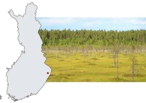
The peatland “Salmisuo” is located at 62◦₄₇′_{N, 30}◦₅₆′_{E, in Eastern Finland (Fig.} ₁_),

20

and is generally classified as an oligotrophic low-sedge pine fen (Saarnio et al.,1997). Climatic conditions represent the boreal forest climate (Strahler and Strahler, 2005) with a mean annual air temperature of + 2.1◦_{C and a mean annual precipitation of}

667 mm (years: 1971–2000 in Finnish Meteorological Institute,2002). The surface of the peatland consists of three main vegetation communities, which follow the

micro-25

topography. Hummocks are elevated and drier areas, (Pinus sylvesteris, Andromeda

(5)

BGD

5, 1097–1117, 2008

Printer-friendly Version Interactive Discussion conditions (Eriophorum vaginatum, Sphagnum balticum, Sphagnum papillosum), and

flarks are wet areas (Scheuchzeria palustris, Sphagnum balticum).

3 Methods

The calculated carbon balance for this study is based on 1) plot-scale quantification of CO2and CH4exchange fluxes using closed chambers over 50 days, 2) a hydrological

5

part to estimate the lateral carbon losses by dissolved organic carbon (DOC) and 3) a remote sensing part to map the spatial distribution of micro-sites.

3.1 Gas flux measurements

For this study, we analyzed CO2and CH4 emission for the time period 26 July 2005–

13 September 2005 (50 days): Fluxes of CO2and CH4were measured with the closed

10

chamber technique (Alm et al.,2007).

Sample plots have been choosen by the three dominant types of micro-sites (flarks, lawns and hummocks). For every micro-site type four replicate sample plots have been used to achieve a representive mean value of the appropriate vegetation type.

CO2 and CH4 fluxes were measured once a week. The CO2 measurements were

15

performed over 24 h. For determination of net ecosystem CO2 exchange, we

em-ployed a vented transparent chamber (60 cm×60 cm×32 cm) with an automatic cooling system which kept the headspace air temperature within approximately 1◦C of the am-bient temperature. The dark respiration and CH4flux measurements were conducted

using vented aluminum chambers. The CO₂ concentrations were measured using a

20

CO2/H2O infrared gas analyzer (LI-840, Licor, USA). CO2 readings were taken at 1 s

intervals over 180 s. During the CH4 flux measurements, four headspace samples

were taken every 4 min from the chamber in a 16 min time period. CH₄ concentra-tion in the syringes were analyzed one day later with a gas chromatograph (Shimadzu 14-A) equipped with a flame ionisation detector. The gas fluxes were calculated from

(6)

BGD

5, 1097–1117, 2008

Printer-friendly Version Interactive Discussion the concentration increase in the chamber headspace over time applying nonlinear

regression for CO₂ (Kutzbach et al.,2007) and linear regression for CH₄. The sea-sonal time series of CO2and CH4exchange fluxes over the investigation period were

modeled on a temporal resolution of 0.5 h for CO2and 1.0 h for CH4using multilinear

regression models with photosynthetically active radiation, air temperature, peat

tem-5

perature in 5 cm, air pressure, wind speed and water table as predictors of CO2fluxes

and groundwater table, peat temperature in steps of 5 cm, 10 cm, 20 cm and 50 cm and wind speed as predictors for CH₄ fluxes. Then, the modeled time series of CO₂ and CH4fluxes were integrated to derive the total amount of CO2and CH4exchanged over

the investigation period. The flux value for each micro-site type was then calculated as

10

the mean of the four replicates. 3.2 Hydrology

Dissolved organic carbon (DOC) export was calculated by multiplying daily surface runoff with average daily DOC mass per volume concentrations ([DOC]); measure-ments were undertaken at a ditch collecting the peatland outflow. [DOC] was

deter-15

mined by daily water sampling and subsequent analysis of UV absorbance at 254 nm in a double beam UV/VIS spectrophotometer. For calibration of the UVVIS spectropho-tometer, a selection of samples was analyzed with a Shimadzu 5000-A TOC analyzer for their [DOC] to establish a linear correlation between UV absorption and [DOC]. Discharge was measured by a sharp-crested v-notch weir. Discharge values were

20

logged every 15 min and subsequently integrated to daily runoff values. The resulting daily DOC flux rates in the stream were converted to export values per unit area (in g C×m–2) through integration over time and then divided by the catchment area size (365 000 m2).

(7)

BGD

5, 1097–1117, 2008

Printer-friendly Version Interactive Discussion 3.3 Remote sensing

The remote sensing task was covered by very high resolution imagery taken from a helium filled dirigible. The dirigible with a volume of 2 m3 was capable to lift 1 kg of payload and was with his tail fins well equipped to be more stable in the air than a balloon. At the bottom of the dirigible, a camera rig was attached that held the camera

5

in an almost nadir position.

To obtain the imagery, we utilized a 7 megapixel point and shoot camera (Canon Powershot G6) combined with a 2 gigabyte storage medium. This setting provided us with the ability to obtain 100 raw data images (*.crw) per flight session with a resolution of 3072×2304 pixels and a shooting frequency of one image per minute. The restriction

10

of 100 images was given by the software of the camera. The ground resolution of these imagery depends very much on the flying height of the platform (e.g. ∼5 cm at a flying height of 130 m above the ground).

For further processing the imagery was georectified using a grid of ground control points (GCPs). The grid had a cellwidth of about 50 m, and the position of every GCP

15

was measured with a differential global positioning system. The average horizontal accuracy of these measurements was 35 cm.

In order to get a reasonable amount of GCPs for georectification and at the same time a very high ground resolution, a flying height of ∼150 m above the ground was chosen, offering a ground resolution of about 6 cm and a minimum of 6 GCPs in every

20

image.

To simulate different flying heights of the dirigible, we coarsened the ground resolu-tion from 6 cm to 10 cm and further in steps of 5 cm up to a resoluresolu-tion of 100 cm. By coarsening the resolution up to 100 cm we cover the range from very high resolution airborne imagery to very high resolution commercial satellite imagery (e.g. QuickBird

25

2 – 61 cm – and IKONOS 2 – 100 cm). Coarsening the resolution was done during the process of georectification in ER Mapper Professional 7.1 of ER Mapper, using the nearest neighbor algorithm to resample the imagery to the desired resolution (Earth

(8)

BGD

5, 1097–1117, 2008

Printer-friendly Version Interactive Discussion Resource Mapping,2006).

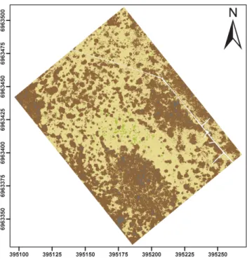
The georectified imagery was classified in the next step, defining regions to represent the micro-site types and using a supervised classification with the maximum likelihood algorithm in ER Mapper 7.1. The resulting land cover map (Fig. 2) was vectorized, using the Raster-To-Polygon function in ArcGIS of ESRI to proceed to the statistical

5

analysis (ESRI,2004).

Furthermore we calculated total area and average size of each micro-site type for each resolution (Table1, Fig.3).

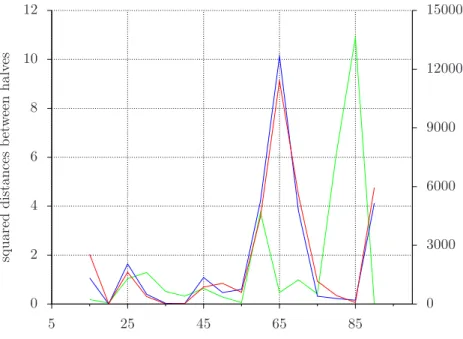
To locate discontinuities in the data we conducted a moving split window analysis (Johnston et al., 1992). Using the moving split window a changing of the observed

10

attribute is indicated by maximum values in the graphs. A four-sample window width was applied to find possible thresholds while coarsening the ground resolution.

4 Results

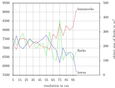
Highest obtained ground resolution was 6 cm and subsequent coarsening resulted in 20 area estimates (Fig. 3) for each micro-site type. Flark area was stable (∼200–

15

250 m2) below a threshold of ∼25 cm and then decreased with coarsening resolution (loss of 54 % between 6 cm and 100 cm) with the exception of the resolution between 55 cm and 80 cm, were values for flarks varied by up to 370 %. Area of lawns and hum-mocks (∼7000–7200 m2) was stable until a threshold of ∼60 cm. Coarser resolutions resulted in a linear increase of hummocks and a concurrent decrease in lawns (21 %

20

change between 6 cm and 100 cm). The oscillation of the values in Fig.3is very likely the effect of a changing pixel pattern when resampling the imagery. Furthermore the selection of the training area for the algorithm and the variety of pixel values within these area adds fluctuations to the graphs. The big fluctuation in the class of flarks be-tween a resolution of 55 cm and 80 cm is showing the unreliability of the data at these

25

resolution. In comparison to these uncertainties Fig.4 is showing a threshold for the class of flarks at a resolution of 60 cm. Due to the small contribution of flarks to the

(9)

BGD

5, 1097–1117, 2008

Printer-friendly Version Interactive Discussion total area, estimates of lawns and hummocks behave nearly as mirror images of each

other (Fig.3). This effect is probably also related to the resampling and classification method. The amount of single objects in the classes of lawns and hummocks and their close spatial relationship is causing a give-and-take between these two classes at their common border. Hence the spatial representation of the two major classes depend on

5

each other and a changing of much smaller classes has no reasonable effect.

Seasonal gas fluxes differed between micro-site types (Tab. 2) with flarks emitting the most CH₄per area and hummocks taking up most of the CO₂per area. Seasonal DOC export was calculated as 0.09 ± 0.02 g C/m2, representing only 0.44 % of the sea-sonal carbon balance. Taken together, the generalizations in lower resolution imagery

10

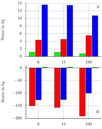
lead to biased area estimates for the individual micro-site types (Fig.3), and thus at a resolution of 100 cm to an overestimation of total CO2 uptake of ∼5.5 % (Fig.5a) and

an underestimation of total CH4emission of ∼11 % (Fig.5b).

The accuracy of gas flux estimations in this approach is highly related to the ground resolution of the imagery used for the classification. Due to stronger generalization at

15

a smaller scale the loss of small objects is increasing by coarsening the pixel size. To identify possible thresholds for the detection of large changes in the calculated area during the coarsening process and thus reasonable object sizes at the particular resolution (Fig. 4), we used the moving split window analysis (MSWA) e.g. Johnston

et al. (1992). For every micro-site the lowest possible detection threshold, indicated by

20

the peak, is located at a ground resolution of 25 cm. The next possible threshold for every micro-site is at a ground resolution of 60 cm.

Based on the results of the MSWA (Fig.4) we calculated the mean object size for every micro-site type at ground resolutions of 25 cm and 60 cm (Table 3) to propose ratios for each micro-site type for the identification of objects in similar heterogeneous

25

environments like the observed peatland (Table4). We have choosen the mean object size to minimize influence of a dominating number of small objects at all resolutions.

(10)

BGD

5, 1097–1117, 2008

5 Discussion

The underestimation of methane fluxes at lower resolution, caused by the underesti-mated area of flarks and lawns, leads to a conservative approximation of the methane fluxes in the particular area. Using a ground resolution of 100 cm the total carbon budget is underestimated by ∼1.18 g/m2in the sample area, compared to the highest

5

resolution of 6 cm. The total amount of effective greenhouse gases would be underes-timated by ∼9.3 % between a ground resolution of 6 cm and 100 cm. Using land-cover maps with even lower resolutions (Takeuchi et al.,2003), would very likely increase this effect.

As shown in Fig. 3 the total area of individual micro-site types, depending entirely

10

on the size and number of the associated polygones, is altered at a changing reso-lution. On the one hand this is caused by the generalization of details from high to lower resolution data (Jensen,2000). On the other hand it is more difficult to identify smaller objects at lower resolutions, leading to errors during the classification process (Markham and Townshend, 1981). It is also possible, that the classification result is

15

influenced by the data distribution, considering that the maximum likelihood algorithm assumes a normal distribution of the band data (Leica Geosystems GIS and Mapping,

2003).

The result of the MSWA indicates possible thresholds for the resolution of the im-agery (Fig.4). To achieve reasonable classification results in a peatland like Salmisuo

20

a ground resolution of 25 cm is recommended to analyze small micro-sites (e.g. flarks). To analyze micro-sites as lawns and hummocks a ground resolution of 60 cm seems to be adequate. Both thresholds show that very high satellite imagery still tends to misjudge the distribution of the micro-sites (plant communities) in small patterned peat-lands.

(11)

BGD

5, 1097–1117, 2008

6 Conclusions

We show that based on differing ground resolution of the land-cover map, substan-tially different areas for individual micro-site types are calculated. This influences the calculation of the carbon balance, since gas fluxes between the ecosystem and the atmosphere are measured at representative spots of each micro-site type and then

5

multiplied by the micro-site area. In particular small micro-sites, which are often bio-geochemical hot-spots, (e.g. wet areas emitting CH4), tend to be affected. In our field

site, a ground resolution of 25 cm seems to be necessary for the detection of these biogeochemical hot-spots with respect to CH₄ emission. A resolution of 60 cm seems sufficient for a representative detection of larger micro-site types as well as with

re-10

spect to CO2 fluxes for all micro-sites types. To successfully detect small micro-site

types (e.g. flarks), we thus recommend a ratio of 1:2 of mean object size to image ground resolution and for larger micro-site types (e.g. lawns and hummocks) a ratio of 1:4.

Acknowledgements. Funding for this study was provided by a Sofja Kovalevskaja Research

15

Award to M. Wilmking. I. Forbrich was supported by a Fellowship from the German Federal Environmental Foundation (DBU). T. Becker was partly supported by the German Academic Exchange Service (DAAD). We thank the Umweltbundesamt for support for Barnim Thees and all colleagues of the “Carbon in Peatlands” Conference in Wageningen for helpful discussions. Futhermore we like to thank A. Roberts of the Simon Fraser University in Burnaby, Canada for

20

the use of his remote sensing laboratory and S. Wolf of the ETH Zurich, Switzerland for the generative and enjoyable discussions.

References

Alm, J., Talanov, A., Saarnio, S., Silvola, J., Ikkonen, E., Aaltonen, H., Nyk ¨anen, H., and Mar-tikainen, P. J.: Reconstruction of the carbon balance for microsites in a boreal oligotrophic

25

(12)

BGD

5, 1097–1117, 2008

Printer-friendly Version Interactive Discussion Alm, J., Shupali, N. S., Tuittila, E. S., Laurila, T., Maljanen, M., Saarnio, S., and Minkkinen, K.:

Methods for determining emission factors for the use of peat and peatlands - flux measure-ments and modelling, Boreal Environmental Research, 12, 85–100, 2007.1100

Bubier, J., Moore, T., Savage, K., and Crill, P.: A comparison of methane flux in a boreal landscape between a dry and a wet year, Global Biogeochemical Cyles, 19, GB1023,

5

doi:10.1029/2004GB002351, 2005.1099

Earth Resource Mapping: ER Mapper Professional 7.1 Tutorial, Earth Resource Mapping, San Diego, CA, 2006. 1102

ESRI: ArcGIS 9 – Geoprocessing Commands, Quick Reference Guide, ESRI, Redlands, CA, 2004. 1103

10

Finnish Meteorological Institute: Climatic Statistics of Finland, 2002.1099

Jensen, J. R.: Remote sensing of the environment: an earth resource perspective, Prentice-Hall Inc., 2000.1105

Johnston, C. A., Pastor, J., and Pinay, G.: Landscape Boundaries: Consequences for Biotic Diversity and Ecological Flows, chap. Quantitative Methods for Studying Landscape

Bound-15

aries, 107–125, Springer-Verlag New York, Inc, 1992.1103,1104

Kutzbach, L., Schneider, J., Sachs, T., Giebels, M., Nyk ¨anen, H., Shurpali, N. J., Martikainen, P. J., Alm, J., and Wilmking, M.: CO₂flux determination by closed-chamber methods can be seriously biased by inappropriate application of linear regression, Biogeosciences, 4, 1005– 1025, 2007,

20

http://www.biogeosciences.net/4/1005/2007/. 1101

Laine, A., Sottocornola, M., Kiely, G., Byrne, K. A., Wilson, D., and Tuittila, E. S.: Estimating net ecosystem exchange in a patterned ecosystem: Example from blanket bog, Agr. Forest Meteorol., 18, 231–243, 2006. 1099

Leica Geosystems GIS and Mapping: Erdas Imagine 8.7 Field Guide, Leica Geosystems GIS

25

and Mapping LLC, Atlanta, GA, 2003. 1105

Markham, B. L. and Townshend, J. R. G.: Land cover classification accuracy as a function of sensor spatial resolution, in: Proceedings 15th International Symposium on Remote Sensing of Environment, 1075–1090, 1981. 1105

Riutta, T., Laine, J., Aurela, M., Rinne, J., Vesela, T., Laurila, T., Haapanala, S., Pihlatie, M.,

30

and Tuittila, E. S.: Spatial Variation in Plant Community Functions Regulates Carbon Gas Dynamics in a Boreal Fen Ecosystem, Tellus B, 59, 838–852, 2007. 1099

(13)

BGD

5, 1097–1117, 2008

Printer-friendly Version Interactive Discussion variation in CH4 emissions and production and oxidation potentials at microsites on an

olig-otrophic pine fen, Oecologia, 110, 414–422, doi:10.1007/s004420050176, 1997.1099

Schimel, D. S. and Potter, C. S.: Biogenic trace gases: measuring emissions from soil and water, chap. Process modelling and spatial extrapolation, pp. 358–383, Blackwell Science, Cambridge, Massachusetts, USA, 1995.1099

5

Strahler, A. and Strahler, A.: Physical Geography: Science and Systems of the Human Envi-ronment, John Wiley & Sons, Inc., 2005. 1099

Takeuchi, W., Tamura, M., and Yasuoka, Y.: Estimation of methane emission from West Sibirian wetland by scaling technique between NOAA AVHRR and SPOT HRV, Remote Sensing of Environment, 21–29, 2003.

10

(14)

BGD

5, 1097–1117, 2008

Table 1. Total area covered by different micro-types; results based on classifications of different resolutions.

resolution flark lawn hummock 6 cm 254 m2 7156 m2 7182 m2 15 cm 255 m2 7087 m2 7500 m2 100 cm 165 m2 5641 m2 9142 m2

(15)

BGD

5, 1097–1117, 2008

Table 2. Seasonal gas fluxes of CH₄and CO₂for every micro-site type, estimated from closed chamber measurements; the DOC value is an estimate for the complete catchment.

flarks lawns hummocks

CH₄–C 4.3±1.8 g/m2 1.9±0.8 g/m2 0.6±0.8 g/m2 CO₂–C 10.6±0.03 g/m2 –17.7±0.05 g/m2 –20.9±0.08 g/m2 DOC export flux 0.09±0.02 g C/m2

(16)

BGD

5, 1097–1117, 2008

Table 3. Mean object size of the different micro-site types at indicated thresholds; see Fig.4. resolution flarks lawns hummocks

25 cm 0.15 m2 0.92 m2 1.12 m2 60 cm 0.70 m2 4.80 m2 4.37 m2

(17)

BGD

5, 1097–1117, 2008

Table 4. Ratio of mean object size to ground resolution; no ratio given for flarks at 60 cm due to determined threshold at 25 cm and unreasonable results at lower resolutions.

resolution flarks lawns hummocks

25 cm 1:2 1:4 1:5

(18)

BGD

5, 1097–1117, 2008

(19)

BGD

5, 1097–1117, 2008

Fig. 2. Result of the maximum likelihood classification at a ground resolution of 6 cm; green=flarks, beige=lawns, brown=hummocks, dark gray=shadow, white=boardwalk and dead trees.

(20)

BGD

5, 1097–1117, 2008

Printer-friendly Version Interactive Discussion 5500 6000 6500 7000 7500 8000 8500 9000 9500 5 15 25 35 45 55 65 75 85 95 0 100 200 300 400 500 ob ject size of h ummo cks and la wns in m 2 ob ject size of flarks in m 2 resolution in cm hummocks flarks lawns

Fig. 3. Estimated total areas for flarks, lawns and hummocks at a stepwise coarsened ground resolution from 6 cm to 100 cm. The size of micro-sites is changing on a wide amplitude with changing resolution. Note different y-axes for hummocks/lawns and flarks, respectively.

(21)

BGD

5, 1097–1117, 2008

Printer-friendly Version Interactive Discussion 0 2 4 6 8 10 12 5 25 45 65 85 0 3000 6000 9000 12000 15000 sq u a re d d is ta n c e s b e tw e e n h a lv e s resolution in cm

Fig. 4. Moving split window analysis of the total area covered by flarks, lawns and hummocks; the distances between the halves of the windows (y-axes) is plotted against the resolution (x-axes); The plot is showing the combined result of all three micro-sites, where the left y-axis belongs to lawn (blue) and hummocks (red) and the right y-axis to the flarks (green). Values on the left axis have to be multiplied by 100 000.

(22)

BGD

5, 1097–1117, 2008

Printer-friendly Version Interactive Discussion 0 2 4 6 8 10 12 14 6 15 100 fl u x es in k g A −200 −150 −100 −50 0 6 15 100 fl u x es in k g resolution in cm B

Fig. 5. Seasonal gas fluxes, calculated for the area of every micro-site type (green=flarks, blue=lawns, red=hummocks) at changing resolutions; (A): seasonal fluxes of CH4–C, grouped

by resolution; at a resolution of 100 cm an underestimation of ∼11 % of the total CH4–C

emis-sion is shown; (B): fluxes of CO₂–C, grouped by resolution; using a resolution of 100 cm instead of 6 cm lead to an overestimation of total CO₂–C uptake of ∼5.5 %