Detecting Triangle Inequality Violations for Internet
Coordinate Systems
Mohamed Ali Kaafar and Franc¸ois Cantin and Bamba Gueye and Guy Leduc
University of Liege, Belgium
Email:{ma.kaafar, francois.cantin, cabgueye, guy.leduc}@ulg.ac.be
Abstract—Internet Coordinate Systems (ICS) have been
pro-posed as a method for estimating delays between hosts without direct measurement. However, they can only be accurate when the triangle inequality holds for Internet delays. Actually Triangle Inequality Violations (TIVs) are frequent and are likely to remain a property of the Internet due to routing policies or path inflation. In this paper we propose methods to detect TIVs with high confidence by observing various metrics such as the relative estimation error on the coordinates. Indeed, the detection of TIVs can be used for mitigating their impact on the ICS itself, by excluding some disturbing nodes from clusters running their own ICS, or more generally by improving their neighbor selection mechanism.
Index Terms—Internet delay measurements, Internet
Coordi-nate Systems, Performance, Triangle inequality violations.
I. INTRODUCTION
Internet Coordinate Systems (ICS) have been used to predict the end-to-end network latency for any pair of hosts among a population without extensive measurements. Several prediction mechanisms have been proposed, e.g., [1], [2], [3]. Example of applications than can benefit from such knowledge include overlay routing networks, peer-to-peer networks, and applica-tions employing dynamic server selection, etc.
These systems embed latency measurements among samples of a node population into a geometric space and assign a network coordinate vector (or coordinate in short) in this geometric space to each node, with a view to enable accurate and cheap distance (i.e. latency) predictions amongst any pair of nodes in the population. Node’s coordinates are determined based on measurements to a set of nodes, called neighbors or reference points (often referred to as landmarks).
Most coordinate systems [1], [2], if not all, assume that the triangle inequality holds for Internet delays. Suppose we have a network with 3 nodes A, B and C, where d(A, C) is 1 ms,
d(C, B) is 2 ms, and d(A, B) is 5 ms, with d(X, Y) denoting the measured delay between X and Y. The triangle inequality is violated because d(A, C) + d(C, B) < d(A, B) end ABC is called a TIV (Triangle Inequality Violation). When ABC is a TIV,AB is always the longest edge (by convention) and is referred to as the TIV base. In fact, triangle inequalities are often violated by Internet delays due to routing policies or path inflation [4], and are likely to remain a property of the Internet for the forseeable future. It is also known that such TIVs [5], [6] degrade the embedding accuracy of any ICS [1], [2], [3]. Some papers consider the removal (or at least the exclusion) of the Triangle Inequality violator nodes from the
system to decrease the embedding distortion [7], [8]. However, we claim that sacrificing even a small fraction of nodes, is not arguable since TIVs are an inherent and natural property of the Internet. Rather than trying to remove them, we consider exploiting them to mitigate their impact on ICS and improve overlay routing.
Since TIVs are inherent to the Internet, it is mandatory to build systems that are TIV-aware [9]. Therefore, it might be exploited by overlay routing to set up end-to-end forwarding paths with reduced latencies, or by nodes participating in an ICS to improve their neighbor selection mechanisms. To improve the neighbors detection mechanisms and mitigate the impact of TIVs on ICS, finding the node pairs that form TIV bases is sufficient [10], [11].
In this paper, we aim at identifying node pairs that are likely to be TIV bases. We characterize these pairs using different metrics such that the Relative Estimation Error (REE) on coordinates. One of our findings is that the REE variance of TIV bases is usually smaller. This can be used to infer TIVs with some confidence without any additional measurement. Consequently, we aim at clusterizing node pairs following their REE variances using Gaussian Mixture Models (GMMs) [12]. GMMs are one of the most widely used unsupervised clus-tering methods where clusters are approximated by Gaussian distributions, fitted on the provided data. We have also applied an AutoRegressive Moving Average (ARMA) [13] model on the sorted REE variances to find a breaking point, because in many practical regression-type we cannot fit one uniform regression function to the data.
The rest of this paper is organized as follows. Sec. II evaluates how TIVs impact the Vivaldi system and introduces our used metric to detect TIV situations. Sec. III explores and evaluates several strategies to infer TIV bases. Finally, Sec. IV summarizes our conclusions and discusses future research directions.
II. VIVALDI ANDTRIANGLEINEQUALITYVIOLATIONS
Internet coordinate systems [1], [2], [3] embed latency measurements into a metric space and associate with each node a coordinate in this metric embedding space. When faced with TIVs, coordinate systems resolve them by forcing edges to shrink or to stretch in the embedding space.
We used two basic characterizations of TIV severity as proposed in [11]. The first one is the relative severity and is defined by Gr= (d(A, B) − (d(A, C) + d(C, B)))/d(A, B).
Relative severity is an interesting metric, but it may be argued that for small triangles, a high relative severity may not be that critical. Therefore we also define a second metric called the absolute severity, which is defined as Ga =
d(A, B) − (d(A, C) + d(C, B)). In the sequel, we will ignore the less important TIVs by considering only those satisfying Ga > 10 ms and Gr> 0.1 [11], and we will omit the “severe”
qualifier. By convention a TIV base is a node pair AB for which there exists at least oneC node so that ABC is a TIV. A non-TIV base is a node pair AB for which there exists no C node so that ABC is a TIV.
A. Vivaldi overview
Vivaldi [2] is an Internet coordinate system based on a simulation of springs, where the position of the nodes that minimizes the potential energy of the spring also minimizes the embedding error. In this system, a new node computes its coordinate after collecting latency information from a few other nodes (its neighbors) only. We choose to focus on Vivaldi because it has many interesting properties: it is fully distributed and requires neither a fixed network infrastructure, nor distinguished nodes. Vivaldi considers a few possible coordinate spaces that might better capture the underlying structure of the Internet e.g.,2D, 3D or 5D Euclidean spaces, spherical coordinates, etc. For the present study, we use a9D Euclidean space and each node computes its coordinates by doing measurements with32 neighbors.
B. Impacts of TIVs on Vivaldi
We used two real data sets to model Internet latencies: the “P2psim” data set, which contains the measured RTTs between 1740 Internet DNS servers, and the “Meridian” data set, which contains the measured RTTs between2500 nodes. Considering the P2psim data set (resp. Meridian), we found that 42% (resp. 83%) of all node pairs are TIV bases.
The authors of [11] show that TIVs impact the performance of Vivaldi, and consequently, the nodes that are the most involved in TIVs have less stable coordinates. Furthermore, the estimated RTT of those nodes pairs are a lot less accurate. In the present study, we do not focus on the nodes and their coordinates but on the node pairs. We define two basic metrics: the Absolute Estimation Error (AEE) and the Relative Estimation Error (REE). Following these two metrics, for a givenAB, we compute:
AEE(AB) = EST (A, B) − RT T (A, B)
REE(AB) = AEE(AB)
RT T (A, B)
where RT T (X, Y ) is the measured RTT between the nodes X and Y and EST (X, Y ) is the estimated RTT obtained with the coordinates of the nodesX and Y .
Wang et al. in [10] show that it exists a relation between the estimation error and the TIV severity. They observed that if a node pair is a TIV base, it is probably shrunk in the metric space. By comparing the RTTs of our two delay matrices to those obtained with Vivaldi (i.e estimated), we found the same
0 5 10 15 20 25 30 35 40 45 50 -200 -150 -100 -50 0 50 100 150 200
Percentage of node pairs
AEE in ms
TIV bases Non-TIV bases
Figure 1. Distribution of the P2psim node pairs in function of AEE.
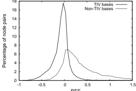
0 2 4 6 8 10 12 14 16 18 -1 -0.5 0 0.5 1 1.5
Percentage of node pairs
REE
TIV bases Non-TIV bases
Figure 2. Distribution of the P2psim node pairs in function of REE.
trend. Indeed, according to the P2psim and Meridian datasets, more than 70% of TIV bases are underestimated (i.e. they have a negative estimation error). For each delay matrix, we clusterize node pairs into two groups: the TIV bases, and the non-TIV bases. Based on the P2psim data set, figures 1 and 2 show the distributions of node pairs with respect to their AEE and REE. We divide the whole range of AEE (resp. REE) into bins equal to 10 ms (resp 0.05).
According to figures 1, 2, we can see that a criterion based on the estimation errors (as proposed in [10]) has a serious drawback: since the overlaping of the two curves is important in each case, it would be difficult to discriminate the TIV bases. Note that the Meridian data set shows similar results with respect to P2psim data set.
Since a detection criterion based on the basic AEE and REE parameters cannot give satisfactory results, we take into account another parameter. Instead of considering the relative estimation error at a fixed time, a simple alternative is to observe its evolution. For instance, the variance is a metric that can characterize the evolution of the REE with respect to time. To implement a TIV basis detection criterion, we compute the REE variances of node pairs during the last 100 ticks of our simulation. We used the P2psim discrete-event simulator [14], which comes with an implementation of the Vivaldi system. Considering the P2psim (resp. Meridian) data set, figure 3 (resp. 4) shows the CDF of the REE variances of the TIV bases and the non-TIV bases. The first observation is that most TIV bases have small REE variances compared to non-TIV bases.
0 0.05 0.1 0.15 0.2 0.25 0.3 0.35 0.4 0.45 0.5 0 0.2 0.4 0.6 0.8 1 REE Variances
CDF Non−TIV basesTIV bases
Figure 3. CDF of the REE variance (P2psim).
0 0.05 0.1 0.15 0.2 0.25 0.3 0.35 0.4 0.45 0.5 0 0.2 0.4 0.6 0.8 1 REE Variances CDF Non−TIV bases TIV bases
Figure 4. CDF of the REE variance (Meridian).
These findings lead to an easy TIV base detection criterion: if a node pair has a low REE variance, it is likely to be a TIV base. Since the non-TIV base curve has a gentle slope on figure 4, such criterion is expected to give very good results (high TPR and low FPR) on the Meridan data set. On the P2psim data set, the results should be less satisfactory. Indeed, we can see on figure 3 that about 25% of the non-TIV bases have small REE variances. This will probably lead to false positives with a detection criterion based on the REE variance. The next section describes such TIV base detection criteria.
III. DETECTINGTIVBASES
In the light of our observations in section II, we propose two methods to detect TIV bases. We consider that each node is maintaining a sliding window (history) of the REE of each link to its ICS neighbors. Each node then computes variances of such REE, and ends up, at each embedding step, with a variance vector y of N entries, N being the number of neighbors the node is considering.
The basic idea behind our detection methods is to differen-tiate variances of TIV bases from variances of non-TIV bases. We aim at creating two separate sets of variances. The set that leads to the minimum mean is likely to contain variances of TIV bases. Next, we will introduce our proposed methods, that we turn into tests to suspect a node pair to be a TIV base. Then, we discuss the performance of our tests in term of false positive and true negative rates.
A. Detection by ARMA models
In this first approach, our objective is to cluster the variances of the REE using the change point detection method. The key idea is to consider a vector of sorted variances as a time series, model such series, and then detect data discontinuities using the model predictions. One of the most suitable models,
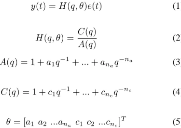
frequently used in system identification and change point detection is the ARMA (AutoRegressive Moving Average) model. Let us consider y(t) as the time series resulting from the sorted vectory. The general form of the ARMA model is as follows [13]: y(t) = H(q, θ)e(t) (1) H(q, θ) = C(q) A(q) (2) A(q) = 1 + a1q−1+ ... + anaq −na (3) C(q) = 1 + c1q−1+ ... + cncq −nc (4) θ = [a1 a2 ...ana c1 c2 ...cnc] T (5)
where q is the shift operator, θ is a vector to describe the time series model, H(q, θ) is a rational function, e(t) is the white noise with varianceσ, A(q) and C(q) are polynomials, na and nc are model orders. Based on the observations up
to time t − 1, the corresponding one-step-ahead prediction of y(t) can be expressed as follows:
ˆ
y(t|θ) = [1 − A(q)]y(t) + [C(q) − 1]ǫ(t|θ) (6) whereǫ(t|θ) is the prediction error, i.e., ǫ(t|θ) = y(t)− ˆy(t|θ). The model parameterθ can be calculated by minimizing the normJN(θ) [13]: ˆ θ(N ) = arg minθ JN(θ) (7) JN(θ) = 1 N N X t=1 l(t, θ, ǫ(t|θ)) (8) where arg min means “the minimizing argument of the func-tion”, andl(t, θ, ǫ(t|θ)) is a scalar-valued function to measure the prediction errorǫ(t|θ). This way of estimating the model parameterθ is called the prediction-error identification method (PEM).
One important advantage of the ARMA model mentioned above is its ability to analyze the time series by breaking them into homogeneous segments, if there are apparent discontinu-ities in the time series. Therefore, it is important to find the time instants when the abrupt changes occur and to estimate the different models for the different segments during which the system does not change. The algorithm that is implemented in this study follows the approach presented in [15], [13], and is based on the following model description:
θ0(t) = θ0(t − 1) + w(t) (9)
where w(t) is zero most of the time, but now and then it abruptly changes the system parameters θ0(t). w(t) is
R1= E[w(t)wT(t)]. For solving this segmentation problem,
a typical Kalman filter algorithm has been given as follows:
ˆ
θ(t) = ˆθ(t − 1) + K(t)ǫ(t) (10) ǫ(t) = y(t) − ˆy(t) = y(t) − ψT(t)ˆθ(t − 1) (11)
K(t) = Q(t)ψ(t) (12) Q(t) = P (t − 1) R2+ ψTP (t − 1)ψ(t) (13) P (t) = P (t − 1) + R1− P (t − 1)ψ(t)ψT(t)P (t − 1) R2+ ψT(t)P (t − 1)ψ(t) (14)
where ˆθ(t) is the parameter estimated at time t, ψ(t) is the regression vector that contains old values of the observations, y(t) is the observation at time t, and ˆy(t) is the prediction of the value y(t) from the observations up to time t − 1 and the current model at time t − 1. ǫ(t) is the noise source with variance, R2 = E[ǫ2(t)]. The gain K(t) determines how the
current prediction error, y(t) − ˆy(t), updates the parameter estimate.
The algorithm is specified byR1, R2, P (0), θ(0), y(t) and ψ(t). R1 is the assumed covariance matrix of the parameter jumps when they occur. Its default value is the identity matrix with the dimension equal to the number of estimated parameters. θ(0) is the initial value of the parameter, which is set to zero. P (0) is the initial covariance matrix of the parameters. Its default is taken to be 10 times the identity matrix. Several Kalman filters are run in parallel to estimate system parameters, each of them corresponding to a particular assumption about when the system actually changes. Each time the algorithm returns the model parameter changes, we log the instants such change occur. Recall that we consider such time series as series of variances of REE. Hence, when a change occurs at time τ , we will consider all y(t), t < τ as variances of the REE of TIV bases. Obviously, changes may be multiple, but to differentiate variances of TIV bases from variances of non-TIV bases, a node will consider only the first change point detected by the model.
B. Detection by GMM clustering
In this section, we adopt a second strategy to detect TIV bases. Rather than modeling the series of variances, we aim at clustering the REE variances into classes where variances in one cluster are close to each other, and clusters are far apart. In such a way, we would be able to identify the cluster that contains the variance with low mean, and report its elements as variances of the REE of TIV bases. Gaussian Mixture Models (GMMs) are among the most statistically mature methods for clustering, and may be more appropriate than other clustering techniques such as K-means, especially because clusters of variances may have different sizes and correlations between them. Although we still need to look for
a differentiation between two main clusters (TIV variances and non-TIV variances), we could distinguish more than two clusters, sayk. This allows the GMM clustering to create more accurate clusters, from which we choose the cluster that is more likely to contain TIV variances.
Given the variance vector y of N entries, clusters are formed by representing the probability density function of observed variances as a mixture of gaussian densities. We use the Expectation Maximization algorithm to assign posteriori probabilities to each component density with respect to each observation (to each variance value in our situation). Clusters are then assigned by selecting the component that maximizes the posteriori probability. We report interested readers to the approach described in [12], and that we used in this work.
More formally, let us consider the variance vector y = (y1, ..., yN) that we would like to cluster. Clusters are
rep-resented by probability distributions, typically a mixture of gaussian distributions. Hence, a clusterC is represented by a mean value of all values in the cluster,µC, and the variance of
values in the cluster, sayP
C. The density function of cluster
C is then: P (y|C) = e (y−µc)2 2.P C p(2π)N.P C (15)
LetWi denote the fraction of cluster Ci in the entire data
set. In this way, we have P (y) = Pk
i=1Wi.P (y|Ci), the
density function for clustering M = C1, ..., Ck. Each point
may belong to several clusters with different probabilities:
P (Ci|y) = Wi.
P (y/Ci)
P (y)
The Expectation Maximization (EM) algorithm, consists then in maximizing E(M ), as a measure of the quality of the clustering M , E(M ) being defined as
E(M ) =X
y
log(P (y))
E(M) indicates the probability that the data have been gen-erated by following the distribution model as defined by M . The clustering process using the Expectation Maximization method consists then in generating an initial model, say M′ = (C′
1, ..., C ′
k), and repeat the assignments of points to
clusters and the computations of the model parameters until the method converges to unstable clustering state maximizing the probability that the data observed follows the distribution model M . Basically, the algorithm (re)computes P (y/Ci),
P (y) and P (Ci|y) for each observation from the dataset and
for each cluster (Gaussian distribution)Ci, then (re)computes
a new model M = (C1, ..., Ck) by recomputing Wi, µC
andP
C for each clusterC (following equations 16, 17, 18).
Finally it replaces the distribution M′ byM .
Such process continues until|E(M ) − E(M′)| < ǫ, where
ǫ is constant defining the convergence of the algorithm. When the EM method converges, it returns the distribution M of clusters.
1 0.9 0.8 0.7 0.6 0.4 0.3 0.2 0.1 0
TPR (True Positive Rate)
FPR (False Positive Rate)
REE < 0 REE < 0.05 REE < 0.1 REE < 0.15 ARMA model GMM model REE detection thresholds
(a) P2psim data set
1 0.9 0.8 0.7 0.6 0.4 0.3 0.2 0.1 0
TPR (True Positive Rate)
FPR (False Positive Rate) REE < 0.2 REE < 0.25 REE < 0.3 REE < 0.35 ARMA model GMM model REE detection thresholds
(b) Meridian data set
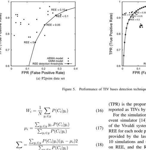
Figure 5. Performance of TIV bases detection techniques.
Wi= 1 N X yi∈y P (Ci|yi) (16) µi= P yi∈yyi.P (Ci|yi) P yi∈yP (Ci|yi) (17) X i = P yi∈yP (Ci|yi)(yi− µi)2 P yi∈yP (Ci|yi) (18)
To select the cluster we suspect to contain variances of TIV bases, we look for the cluster corresponding to min1<i<kµi. C. Detection Results
To characterize the performance of our detection tests, we use the classical false/true positive/negative indicators. Specifically, a negative is a non-TIV base, which should therefore not be reported in the set of suspects that we derive. A positive is a TIV base, which should therefore be suspected by the test.
A false negative is a TIV base that has been wrongly classified by the test as negative, and has therefore been wrongly unsuspected. A false positive is a non-TIV base that has been wrongly suspected by the test. True positives (resp. true negatives) are positives (resp. negatives) that have been correctly reported by the test and therefore have been rightly suspected (resp. unsuspected). The number of false negatives (resp. false positives, true negatives and true positives) reported by the test isTF N (resp.TF P,TT N andTT P).
We use the notion of false negative rate (FNR) which is the proportion of all TIV bases that have been wrongly reported as non-TIVs by the test, and FNR = TF N/PP. The number
of negatives (resp. positives) in the population comprising all the links between a node and its neighborhood is PN (resp.
PP). The false positive rate (FPR) is the proportion of all the
non-TIV bases that have been wrongly reported as positive by the test, soFPR = TF P/PN. Similarly, the true positive rate
(TPR) is the proportion of TIV bases that have been rightly reported as TIVs by the test, and we haveTPR = TT P/PP.
For the simulation scenarios, we used the P2psim discrete-event simulator [14], which comes with an implementation of the Vivaldi system and each node has 32 neighbors. The REE for each node pairs is computed based on the coordinates provided by the last tick of our simulation. We performed 10 simulations and used different detection thresholds based on REE, and the Receiver Operating Characteristic (ROC) curve obtained for one simulation is presented on figures 5(a) and 5(b) respectively for the P2Psim and Meridian data sets. Since we observed the same trend for all ROC curves only one ROC curve is depicted on figures 5(a) and 5(b). We consider different thresholds varying from −1 to 1 by steps of 0.05. Each point on the ROC curves determines the TPR and the FPR obtained with a given detection threshold. For instance, considering the curve obtained with the detection thresholds based on REE, different REE values are illustrated on figure 5. Note that a REE threshold lower than0 means a underestimation of the actual distance, whereas a REE greater than0 expresses an overestimation.
We experimented withna= 1 and nc= 1 as model orders
of the ARMA modeling detection technique, while we set k = 4 as number of mixtures in the GMM clustering tech-nique. The reader should note though that we experimented with different parameters of our detection methods that lead to similar or better results. The plot in figure 5 shows the points corresponding to the false positive rates along the x-axis and to the true positive rates along the y-x-axis, with one point per method used to detect TIV bases, for both data sets with respect to 10 simulations results. By considering ARMA and GMM models we don’t need to set any threshold.
Obviously, the closer to the upper left corner of the graph a point is, the better, since such points correspond to high true positive rates (i.e. a high proportion of positives being reported as such by the test) for low false positive rates (i.e. a small proportion of negatives incorrectly reported as positives).
The first observation on figure 5 is that the REE thresholds which give high TPR with low FPR are different for the P2psim and Meridian data sets. The better REE thresholds, when one considers P2psim data set (resp. Meridian data set), vary from0 to 0.15 (resp. 0.2 to 0.35). In other words, a good REE threshold depends on the used data set, and thus, it will be difficult to fix it a priori.
We observe that both detection methods perform very well for the King dataset (figure 5(a)) comparatively to the ROC curve based on REE detection threshold which is the method proposed in [10]. Note that the ARMA model gives better results than GMM model. Furthemore, the two points that are located at the right of the ROC curve (figure 5(a)) represent the detection of TIV bases based on GMM model. The same trend is observed on figure 5(b) where all the detection of TIV bases based on GMM model are located at the right of the ROC curve. Nevertheless, the ARMA model can be considered to be excellent in the case of the Meridian data set.
In summary, the detection of TIV bases based on ARMA model gives good performance with up to 85% of TIV bases detected, while suspecting non-TIV bases in rare situations (less than 2%). The reason that ARMA model outperforms the GMM model is probably due to the fact that the REE variances don’t follow a gaussian distribution.
IV. CONCLUSION
In this paper, we have observed that TIV bases have usually a small REE variance. Following that, we clusterized the REE variance of node pairs using GMMs and ARMA models. We obtained satisfactory results with up to 85% of TIV bases detected, while suspecting non-TIV bases in rare situations. However, these results have been computed considering simulations of Vivaldi: in practice the RTTs are not constant and the detection results could be mitigated. Moreover, in ICS applying such detection criteria on the same set continuously can lead to a degradation of the detection performance. Indeed, this criterion is based on the assumption that TIVs are measured in the ICS and that they impact the ICS behaviour. If we use the result of the detection criterion to optimize the selection of neighbors to reduce the impact of TIVs we will modify the behavior of the ICS. Consequently, the FPR can increase while the TPR decreases at the same time. To avoid such drawback, one solution is to ignore the results of detection if most node pairs are considered as TIV bases.
We believe these TIV bases detection techniques serve as a first step towards a TIV-aware systems. Indeed, we can turn TIV detection into a routing advantage [16], knowing that a TIV means the existence of a shortcut path between the two nodes linked by the longest edge of the “triangle”.
ACKNOWLEDGMENTS
This work has been partially supported by the EU un-der projects FP6-FET ANA (FP6-IST-27489) and FP7-Fire ECODE (FP7-223936).
Franc¸ois Cantin is a Research Fellow of the Belgian Fund for Research in Industry and Agriculture (FRIA).
REFERENCES
[1] T. S. E. Ng and H. Zhang, “Predicting Internet network distance with coordinates-based approaches,” in Proc. IEEE INFOCOM, New York, NY, USA, June 2002.
[2] F. Dabek, R. Cox, F. Kaashoek, and R. Morris, “Vivaldi: A decentralized network coordinate system,” in Proc. ACM SIGCOMM, Portland, OR, USA, Aug. 2004.
[3] M. Costa, M. Castro, R. Rowstron, and P. Key, “Pic: practical internet coordinates for distance estimation,” in Proc. the ICDCS, 2004, pp. 178– 187.
[4] H. Zheng, E. K. Lua, M. Pias, and T. Griffin, “Internet Routing Policies and Round-Trip-Times,” in Proc. the PAM Conference, Boston, MA, USA, Apr. 2005.
[5] S. Lee, Z. Zhang, S. Sahu, and D. Saha, “On suitability of euclidean embedding of internet hosts,” SIGMETRICS, vol. 34, no. 1, pp. 157–168, 2006.
[6] E. K. Lua, T. Griffin, M. Pias, H. Zheng, and J. Crowcroft, “On the accuracy of embeddings for internet coordinate systems,” in Proc the
IMC Conference. New York, NY, USA: ACM, 2005, pp. 1–14.
[7] J. Ledlie, P. Gardner, and M. I. Seltzer, “Network coordinates in the wild,” in Proc NSDI, Cambridge, apr 2007.
[8] Y. Bartal, N. Linial, M. Mendel, and A. Naor, “On metric ramsey-type phenomena,” in Proc. the Annual ACM Symposium on Theory of
Computing (STOC), San Diego, CA, june 2003.
[9] Y. Lia, M. A. Kaafar, B. Gueye, F. Cantin, P. Geurts, and G. Leduc, “Detecting triangle inequality violations in internet coordinate systems by supervised learning,” in Proc. IFIP Networking Conference, Aachen, Germany, May 2009.
[10] G. Wang, B. Zhang, and T. S. E. Ng, “Towards network triangle inequality violation aware distributed systems,” in Proc. the ACM/IMC
Conference, San Diego, CA, USA, oct 2007, pp. 175–188.
[11] M. A. Kaafar, B. Gueye, F. Cantin, G. Leduc, and L. Mathy, “Towards a two-tier internet coordinate system to mitigate the impact of triangle inequality violations,” in Proc. IFIP Networking Conference, ser. LNCS 4982, Singapore, May 2008, pp. 397–408.
[12] G. J. McLachlan and D. Peel, Finite Mixture Models. New York, MA: Wiley, 2000, vol. 1.
[13] L. Ljung, System identification toolbox for use with Matlab-users guide, The MathWorks, Inc., Natick, Mass., 1995.
[14] A simulator for peer-to-peer protocols, http://www.pdos.lcs.mit.edu/ p2psim/index.html.
[15] J. Li, K. Miyashita, T. Kato, and S. Miyazaki, “Gps time series modeling by autoregressive moving average method,” in Earth Planets Space, vol. 52, 2000, p. 155.
[16] F. Cantin, B. Gueye, M. A. Kaafar, and G. Leduc, “Overlay routing using coordinate systems,” in Proc. ACM CoNEXT Student Workshop, Madrid, Spain, Dec. 2008.