EUREC4A-OA_OCARINA : OCARINA Air-Sea Flux Data

HAL Id: hal-03066519

https://hal.archives-ouvertes.fr/hal-03066519

HAL is a multi-disciplinary open access archive for the deposit and dissemination of sci-entific research documents, whether they are pub-lished or not. The documents may come from teaching and research institutions in France or abroad, or from public or private research centers.

L’archive ouverte pluridisciplinaire HAL, est destinée au dépôt et à la diffusion de documents scientifiques de niveau recherche, publiés ou non, émanant des établissements d’enseignement et de recherche français ou étrangers, des laboratoires publics ou privés.

EUREC4A-OA_OCARINA : OCARINA Air-Sea Flux

Data

Denis Bourras, Hubert Branger, Luneau Christopher, Gilles Reverdin, Sabrina

Speich, Geykens Nicolas, Hervé Barrois, Aurélien Clémençon

To cite this version:

Denis Bourras, Hubert Branger, Luneau Christopher, Gilles Reverdin, Sabrina Speich, et al.. EUREC4A-OA_OCARINA : OCARINA Air-Sea Flux Data. 2020, �10.17882/77479�. �hal-03066519�

EUREC4A experiment: Air-Sea OCARINA Data

Denis Bourras1,Hubert Branger1,2, Christopher Luneau3, Gilles Reverdin4

Sabrina Speich5, Nicolas Geyskens6, Hervé Barrois6, and Aurélien Clémençon6

1

MIO, Mediterranean Institute of Oceanology, Marseille, France

2

IRPHE, Marseille, France

3

OSU Pytheas UMS 110, Marseille, France

4

LOCEAN, Paris, France

5

LMD, ENS, Paris, France

6

DT-INSU Meudon, France

Technical report LASIF 2020-04DB 08 December 2020

Version 0.5

1. Introduction

In the context of the EUREC4A-OA oceanographic cruise

(https://campagnes.flotteoceanographique.fr/campagnes/18000670/), the OCARINA platform (Bourras et al., 2014, 2019) was deployed four times from the host Research Vessel (R/V) Atalante from Genavir. The location of the deployments is close to the Barbados Island (Bourras et al. 2020, https://www.seanoe.org/data/00661/77341/data/78808.pdf).

The OCARINA platform is a small 2 m-long ship that was specifically designed to estimate air-sea turbulent and radiation fluxes, as well as sea surface characteristics. During EUREC4A, OCARINA was used as a drifting buoy.

The measured quantities are:

 Wind vector u, v, w (m/s) and speed of sound c (m/s) at 50 Hz, by a Gill R3‐50, at a height of 1. 6 m

 Air temperature T (°C), relative humidity RH (%), and atmospheric pressure Patm (hPa) at 1 Hz, by a Vaisala WXT‐520 instrument, at a height of 0.8 m.

 Solar and infrared radiation fluxes, upward and downward: Fsol_dn, Fsol_up, Fir_dn, and

Fir_up (W/m2 ), at 1 Hz, by a Campbell CNR4, at a height of 0.8 m

 Time, position, and motion: lon (°), lat (°), lin_acc_xyz (m/s2 ), ang_vel_xyz (rad/s), and Euler angles (phi, theta, psi) at 50 Hz, by a Xsens MTI‐G, at a height of 0.1 m

 Sea temperature and salinity: SST (°C) and SSS (psu) at 1 Hz, by a Seabird SBE‐37SI probe, at a depth of 0.3 m

The algorithm used for processing the turbulent fluxes and quantities (Albatros code) is publicly available at https://gitlab.osupytheas.fr/bourras.d/albatros_public_distrib, and it was described in Bourras et al. (2019). Three methods are used to estimate the fluxes: the Eddy-Covariance (EC) method, the Inertial-Dissipation (ID) method, and the Bulk (COARE 3.0 code by Fairall et al., 2003) method, with the parameterization of the roughness length by Smith (1988). The fluxes under analysis in the present report are specifically the friction velocity u* (in m/s), and the turbulent buoyancy flux Hsv (in W/m2).

The report is organized as follows. In section 2, the specific aspects of the EUREC4A processing are presented. Next, in section 3, the power spectra and the co-spectra of wind and virtual temperature are presented and are compared to reference data, and two frequency ranges are selected for the inertial turbulent sub-range. In section 4, the two sub-ranges are tested, i.e. the u* values obtained with the two sub-ranges are compared and the turbulent dissipation rates for wind and temperature are also compared. In section 5, several calculation options of the Albatros code are tested. Next, a mean correction of the EC u* values is proposed and an imbalance term is proposed for correcting ID u* values. Conclusions follow in section 6.

2. Improvement of the Albatros code

The flux calculation process has several stages. One of these is the true wind calculation, which includes a rotation of the measured wind vector, from the Gill R3-50 local coordinate system to an Earth referenced coordinate system. Rotation is done according to the Euler angles measured by the Xsens MTI-G data.

While processing the EUREC4A-OCARINA data, we noticed that the psi angle measured by the MTI-G instrument could not be used to efficiently rotate the wind vector at a high sampling rate (i.e. at 32 Hz in the Albatros code). Indeed, after rotation at 32 Hz, the time series of the u-wind component have outlier data (Figure 1, left panel). In response, a median filter was applied to smooth the time series of psi data at 1 Hz. The wind data corrected at 1 Hz present no outliers, which means that the filtering is efficient (Figure 1, right panel). Please note that the filtering was done per axis (in sine and in co-sine) as psi is an angle.

Figure 1. Superimposition of all the 1 100 second time series of the longitudinal wind component, for the first day of the experiment. The yaw (psi) rotation was applied either at 32 Hz (left panel) or at 1

Hz (right panel). On the left panel, there are outlier points that correspond to wind speed values smaller than 2 m/s. These points did not appear in the original time series (before yaw rotation was

applied), which is not shown here. After smoothing at 1 Hz (right panel), the outliers disappear. Note also that with the original 32 Hz correction, there is a large negative impact of the outlier points in terms of spectral slope. Indeed, the individual wind spectra multiplied by f5/3 increase with frequency, thus they do not follow the expected -5/3 theoretical Kolmogorov log-log slope (Figure 2). With the new 1 Hz psi rotation, the spectra are well corrected (please see section 3).

3. Spectral analysis

3.1 Power spectra

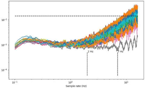
With the 1 Hz-psi rotation (section 2), the averaged power spectra of the u-wind component reasonably follow a -5/3 log-log slope between 2 and 4 Hz (Figure 3), which means that this frequency range may be reasonably selected to calculate ID fluxes.

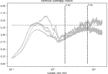
Figure 3. Daily power spectra of the along-mean wind component with the 1 Hz psi rotation In theory, the vertical isotropy Ew(f)/Eu(f) should average to 4/3 in the inertial sub-range. The EUREC4A data noticeably differ from this value (Figure 4), with values in the range 0.8-1. This discrepancy is more marked in the [ 2 ; 4] Hz inertial sub-range that was selected above. As the vertical isotropy is closer to 4/3 in the [ 4 ; 7 ] Hz frequency range, the two sub-ranges will be tested in the next section for ID calculation.

Figure 4. Vertical isotropy per day of the experiment. The 4/3 theoretical value is highlighted by the horizontal dashed line.

The value of the horizontal isotropy is close to 4/3 at 4 Hz (Figure 5). It averages to 1.3 in the range [ 2 ; 4 ] Hz, and it is 1.4 in average, in the range [ 4 ; 7 ] Hz, which is acceptable.

Figure 5. Horizontal isotropy per day of the experiment. The 4/3 theoretical value is denoted by the horizontal dashed line.

The power spectra for the virtual temperature are presented in Figure 6. Only one out of the four daily spectra adequately follows a -5/3 slope. The three other spectra multiplied by f5/3 increase with frequency. This behavior of the temperature spectrum was already noticed for other experiments (Bourras et al., 2019), for which it was noticed that it depended at least on wind speed, although it was not fully understood. Note that there are no obvious outliers in the corresponding time series of virtual temperature (Figure 7), as was previously noted for wind data (Figure 1).

Figure 7. Example of time series of virtual air temperature during EUREC4A

3.2 Co-Spectra

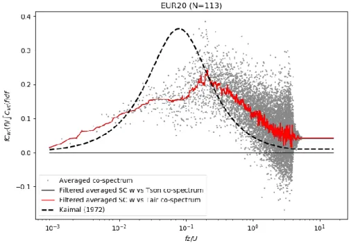
The u-wind versus w-wind co-spectrum Cu’w’(f) has a bell shape that is approximately centered on co-spectrum modeled by Kaimal et al. (1972), as shown in Figure 8. However, there is less energy in the EUREC4A co-spectrum than in the Kaimal et al. (1972) co-spectrum, which indicates that, the subsequent EC u* estimates could be under-estimated. The maximum frequency of the peak of energy is located at larger frequencies than the Kaimal et al. (1972) model, as in Bourras et al. (2019). In the Albatros code, there are three options for correcting the w-wind component from the platform vertical motion. By default, a spectral method is used. However, it is also possible to apply a direct subtraction method or no correction at all (Bourras et al., 2019). For the EUREC4A data set, we note that the application of a vertical wind correction decreases the value of the energy peak (Figure 8). It suggests that a correction of the vertical velocity will accentuate the under-estimation of the EC u* estimates (see section 5).

Figure 8. Longitudinal versus vertical wind co-spectrum

The wind-temperature co-spectrum Cw’t’(f) has comparable characteristics, which consists in (1) a bell-shape and (2) less energy than in the Kaimal et al. (1972) reference co-spectrum (Figure 9).

Figure 9. Vertical wind versus virtual temperature co-spectrum

4. Wind inertial sub-range

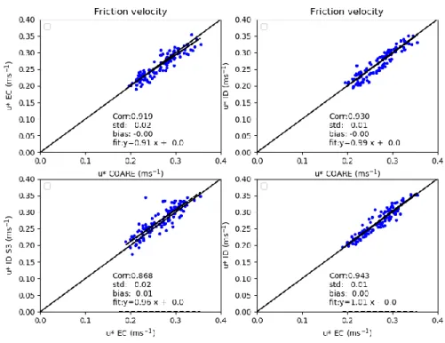
We estimated the friction velocity with the two [ 2 ; 4 ] Hz and [ 4 ; 7 ] Hz test sub-ranges defined in section 3.1. The comparisons between u* calculated with the EC, ID, and bulk methods are reported in Table 1. The comparison between u* ID and u* bulk is improved with the [ 4; 7 ] Hz range, as the slope of linear fit increases from 0.76 to 0.85. In addition, the comparison between u* ID and u* EC is also improved (slope from 0.78 to 0.86). The comparison between u* ID S3 and u* EC is slightly degraded, specifically in terms of slope of linear fit (from 0.9 to 0.8). Therefore, based on Table 1 results only, the choice of the [4 ;7] Hz sub-range may be discussed. However, the comparison of dissipation rates based on power spectra and to third order structure functions also suggests that it is a better choice, as the results clearly comply with Bourras et al. (2019) findings when the [4 ; 7] Hz range is selected.

u* comparison Correlation  Bias Slope of linear fit

ID [2 ;4] Hz -bulk 0.922 0.02 -0.05 0.76 ID [4 ;7] Hz -bulk 0.933 0.01 -0.04 0.85 ID S3 [2 ;4] Hz – EC 0.884 0.02 -0.01 0.90 ID S3 [4 ;7] Hz – EC 0.868 0.02 -0.02 0.80 ID [2 ; 4] Hz –EC 0.938 0.01 -0.03 0.78 ID [4 ; 7] Hz –EC 0.942 0.01 -0.02 0.86

Table 1. Comparison of friction velocity estimates for two ranges of frequencies

Indeed, with the [4 ;7] Hz range, the agreement between dissipation rates is improved (compare panels a in Figures 10,11), like in Bourras et al. (2019, Figure 7). The same occurs for the half destruction rates of temperature variance (panels d in Figures 10,11). This also confirms that for wind, the mean value of the third-order structure function for wind dissipation has to be considered, while the maximum value has to be accounted for, for temperature, like in Bourras et al. (2019). Note finally that the changes for the buoyancy flux Hsv are negligible (not shown).

Figure 10. Dissipation rate comparison for wind and temperature, when the [2;4] Hz range is selected

Figure 11. Dissipation rate comparison for wind and temperature, when the [4;7] Hz range is selected

5. Turbulent quantities

5.1 Fluxes

The calculation of the turbulent fluxes (u* and Hsv) depends on many options, several of which are tested in this section.

The initial reference run (with the [2;4] Hz range) gives the comparison statistics reported in Table 2. u* EC is underestimated by -0.02 m/s with respect to u* bulk, and EC Hsv values are also under estimated with respect to their bulk counterpart, by -6.3 W/m2.

u* comparison Correlation  bias Slope of linear fit

EC-bulk 0.919 0.02 -0.02 0.91

ID-bulk 0.920 0.02 -0.05 0.75

ID S3 – EC 0.887 0.02 -0.01 0.92

ID-EC 0.940 0.01 -0.02 0.77

HSv comparison Correlation  bias Slope of linear fit

EC-bulk 0.948 1.68 -6.30 0.78

ID-bulk 0.878 2.65 -6.24 0.56

ID S3 – EC 0.946 1.39 -0.42 0.79

ID-EC 0.846 2.19 0.06 0.65

Table 2. Comparison of u* and Hsv obtained with three estimation methods, for the reference run

5.2 Calculation options

In this section, u* and Hsv are calculated by switching on and off several Albatros options. The resulting comparisons are summarized in Tables, in which the values can be compared to Table 2 values.

 The test of distortion correction, i.e. accounting for the vertical wind angle slightly improves the comparison between u* ID and u* EC and between u* ID S3 and u* EC. In contrast, the comparisons to the bulk u* values are slightly degraded:

u* comparison Correlation  bias Slope of linear fit

EC-bulk 0.919 0.02 -0.02 0.91

ID-bulk 0.920 0.02 -0.05 0.75

ID S3 – EC 0.887 0.02 -0.01 0.92

ID-EC 0.940 0.01 -0.02 0.77

 Accounting for free convection (icnvl=1) in the bulk algorithm produces the adverse effect: comparisons to the bulk are slightly improved:

u* comparison Correlation  bias Slope of linear fit

EC-bulk 0.924 0.01 -0.02 0.92

ID-bulk 0.922 0.02 -0.05 0.76

ID S3 – EC 0.884 0.02 -0.01 0.90

ID-EC 0.938 0.01 -0.03 0.78

 Accounting for radiation fluxes in the bulk algorithm (options jwam=1 and jcool=1) has a negligible impact on u* bulk estimates:

u* comparison Correlation  bias Slope of linear fit

EC-bulk 0.924 0.01 -0.02 0.92

ID-bulk 0.921 0.02 -0.05 0.76

ID S3 – EC 0.884 0.02 -0.01 0.90

ID-EC 0.938 0.01 -0.03 0.78

In contrasts, the bulk Hsv estimates compare better to the other estimates in slope and bias if the radiation fluxes are accounted for:

HSv comparison Correlation  bias Slope of linear fit

EC-bulk 0.954 1.39 -2.80 0.85

ID-bulk 0.849 2.51 -2.74 0.58

ID S3 – EC 0.946 1.39 -0.42 0.79

ID-EC 0.846 2.19 0.06 0.65

 The vertical wind correction applied in the reference run is a spectral correction. The results obtained for the u* EC estimated with a direct subtraction correction are not very different (not shown). However, interestingly, if no correction is applied, the bias of the u* EC cancels. As a counterpart, the correlation between EC and bulk values is smaller, and the standard deviation of the difference is increased.

u* comparison Correlation  Bias Slope of linear fit

EC-bulk 0.901 0.02 0.00 0.96

ID-bulk 0.922 0.02 -0.05 0.76

ID S3 – EC 0.904 0.02 -0.03 0.87

ID-EC 0.941 0.01 -0.05 0.74

As a result, the application of the vertical wind correction is in question. The impact of the correction of the vertical wind component is to decrease the energy of the co-spectrum, thus it possibly produces under estimated u* EC values. In doubt, the spectral correction will be applied in the following and a mean correction of +0.02 m/s will be added to the EC estimates. This is opposed to the +0.01 m/s mean correction found in Bourras et al. (2019). Here, the proposed correction of the EC bias is somewhat arbitrary, but it is intended to reconcile the EC and the already well validated bulk u* values.

5.3 ID u* correction (Imbalance term)

With the mean +0.02 m/s correction applied to the EC estimates, we may now estimate the imbalance term in the TKE equation (Figure 12).

The imbalance term averaged to 0.38, which is close to the value of 0.4 found by Bourras et al. (2019).

If the +0.02 m/s correction is applied to the u* EC estimates and if the 0.38 imbalance term is accounted for, we obtain the comparisons of Figure 13, which are good.

Figure 13. Comparison of corrected u* estimates For Hsv, we obtain the following comparisons (Figure 14).

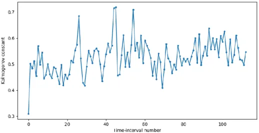
5.4 Constants

The Kolmogorov constant ck averages to 0.53 (the reference value is 0.55). The time series of ck estimates are consistent during the experiment, as shown in Figure 15.

Figure 15. Estimates of the Kolmogorov constant

The Corrsin constant for virtual temperature ct averages to 1.13. The median value is 0.91, which is 12% larger than the reference 0.8 value. The ct values at the end of the experiment are largely overestimated (Figure 16), which is not explained at this time. If they are not considered in the calculation, the average of ct is 0.9.

Figure 16. Estimates of the Corrsin constant

6. Conclusions

The rotation around the vertical axis (yaw) of the measured wind vector cannot be done at 32 Hz with EUREC4A data. Instead, the time series of the yaw angle have to be smoothed at 1 Hz. If it is not done, the subsequent power spectra of the u-wind component are affected and do not follow a -5/3 Kolmogorov log-log slope.

Two corrections of the w-wind component were tested (spectral and direct subtraction), to correct data from vertical platform motion. The application of the corrections was found to underestimate

the energy in the wind co-spectra and to underestimate the values of EC u* compared to bulk u* values. In response, a correction of +0.02 m/s was proposed to reconcile the EC u* values to the bulk estimates. Such a correction means that bulk fluxes are considered as a reference, which is not an issue as long as no parameterizations of roughness length or of the drag coefficient are proposed. The choice of the frequency range considered as the usable inertial turbulent sub-range strongly affects the value of the imbalance term in the ID flux calculation method. Two sub-ranges were tested for the wind, namely [ 2 ; 4 ] Hz and [ 4 ; 7 ] Hz. The second sub-range was a better compromise in terms of (1) deviation to the -5/3 Kolmogorov slope, (2) deviation to the vertical isotropy (4/3), (3) bias between EC, ID, and bulk u* values, and (4) deviation of the turbulence dissipation rates with respect to earlier results by Bourras et al. (2019).

With the [ 4 ; 7 ] Hz range chosen, and with the +0.02 m/s EC u* correction, the imbalance term of the ID flux calculation method averages to 0.38, which is satisfying as it is close to the 0.4 value found in Bourras et al. (2019) with six data sets.

The virtual temperature power spectra generally do not follow a -5/3 log-log slope, which was already noted in Bourras et al. (2019). The inertial sub-range for temperature, chosen as a compromise, is [ 1 ; 2 ] Hz. The resulting ID Hsv estimates do not perfectly compare to bulk or to EC Hsv estimates. However, the ID S3 Hsv estimates (calculated with third-order structure functions instead of power spectra) have a good fit to EC Hsv values. Note that Fairall et al. (1996) already also used third-order structure functions in their study.

The Kolmogorov and Corrsin constants were calculated and average to 0.53 and 0.9, respectively, which is consistent with the 0.55 and 0.8 reference values. However, for the last deployment of OCARINA, the Corrsin constant was largely overestimated by the EUREC4A-OA OCARINA data, which is not yet elucidated.

The ongoing work at MIO is mainly focused on the analysis of the deviation of the temperature power spectrum from a -5/3 log-log slope, as a function of environmental conditions (wind, sea state and stability).

7. References

Bourras, D., Branger, H., Reverdin G., Marié, L., Cambra, R., Baggio, L., Caudoux, C., Caudal, G., et al. (2014). A new platform for the determination of Air-sea Fluxes (OCARINA): overview and first results. Journal of Atmospheric and Oceanic Technology, 31, 1043–1062. https://doi.org/10.1175/JTECH-D-13-00055.1

Bourras Denis, Cambra Remi, Marié Louis, Bouin Marie-Noëlle, Baggio Lucio, Branger Hubert, Beghoura Houda, Reverdin Gilles, Dewitte Boris, Paulmier Aurélien, Maes Christophe, Ardhuin Fabrice, Pairaud Ivane, Fraunié Philippe, Luneau Christopher, Hauser Danièle (2019). Air-Sea Turbulent Fluxes From a Wave-Following Platform During Six Experiments at Sea. Journal Of Geophysical Research-oceans, 124(6), 4290-4321. Publisher's official version : https://doi.org/10.1029/2018JC014803 , Open Access version : https://archimer.ifremer.fr/doc/00503/61436/

Fairall, C. W., E. F. Bradley, D. P. Rogers, J. B. Edson, and G. S. Young (1996), Bulk parameterization of air-sea fluxes in TOGA COARE, J. Geophys. Res., 101, 3,747-3,767.

Fairall. C. W., Bradley, E. F., Hare, J. E., Grachev, A. A., & Edson, J. B. (2003). Bulk Parameterisations of Air-Sea Fluxes: Updates and Verification for the COARE Algorithm. Journal of Climate, 16, 571-591. https://doi.org/10.1175/1520-0442(2003)016%3C0571:BPOASF%3E2.0.CO;2

Kaimal, J. C., Wyngaard, J. C., Izumi, Y., & Coté, O. R. (1972). Spectral Characteristics of surface-layer turbulence. Quarterly Journal of the Royal Meteorological Society, 98, 563-589. https://doi.org/10.1002/qj.49709841707

Smith, S. D. (1988). Coefficients for sea surface wind stress, heat flux, and wind profiles as a function of wind speed and temperature. Journal of Geophysical Research: Oceans, 93(C12), 15467–15472. https://doi.org/10.1029/JC093iC12p15467

8. Data set

netcdf OCARINA_EUREC4A_2020_Proto1_L2_data_20201208_1134 { dimensions:

time = UNLIMITED ; // (2042 currently) variables:

double Time(time) ;

Time:units = "seconds since 2020-1-1 00:00:0.0" ; Time:time_origin = "2020-1-1 00:00:0.0" ; Time:long_name = "time" ; Time:calendar = "gregorian" ; Time:axis = "T" ; Time:_CoordinateAxisType = "Time" ; double lon(time) ; lon:long_name = "longitude" ; lon:standard_name = "longitude" ; lon:units = "degrees_east" ; double lat(time) ; lat:long_name = "latitude" ; lat:standard_name = "latitude" ; lat:units = "degrees_north" ; double pair(time) ;

pair:long_name = "Air pressure" ; pair:standard_name = "air_pressure" ; pair:units = "hPa" ;

double tair(time) ;

tair:long_name = "Air Temperature" ; tair:standard_name = "air_temperature" ; tair:units = "degC" ;

double hur(time) ;

hur:long_name = "Relative air humidity" ; hur:standard_name = "relative_humidity" ; hur:units = "1" ;

double sst(time) ;

sst:long_name = "SST" ;

sst:units = "degC" ; double rho(time) ;

rho:long_name = "Density of air" ; rho:standard_name = "air_density" ; rho:units = "kg m-3" ;

double rlds(time) ;

rlds:long_name = "downwelling longwave radiation flux, positive downward" ; rlds:standard_name = "surface_downwelling_longwave_flux_in_air" ;

rlds:units = "W m-2" ; double rlus(time) ;

rlus:long_name = "upwelling longwave radiation flux, positive upward" ; rlus:standard_name = "surface_upwelling_longwave_flux_in_air" ; rlus:units = "W m-2" ;

double rsds(time) ;

rsds:long_name = "downwelling shortwave radiation flux, positive downward" ; rsds:standard_name = "surface_downwelling_shortwave_flux_in_air" ;

rsds:units = "W m-2" ; double rsus(time) ;

rsus:long_name = "upwelling shortwave radiation flux, positive upward" ; rsus:standard_name = "surface_upwelling_shortwave_flux_in_air" ; rsus:units = "W m-2" ;

double wdir(time) ;

wdir:long_name = "Direction of the wind vector with respect to ground, measured positive clockwise from due north" ;

wdir:standard_name = "wind_to_direction" ; wdir:units = "degrees" ;

double wspd(time) ;

wspd:long_name = "Magnitude of wind velocity with respect to ground" ; wspd:standard_name = "wind_speed" ;

wspd:units = "m s-1" ; double u10n(time) ;

u10n:long_name = "Equivalent neutral wind extrapolated at a 10-m height, from eddy-covariance calculation" ;

u10n:standard_name = "neutral_10m_wind_speed" ; u10n:units = "m s-1" ;

double hsw(time) ;

hsw:long_name = "Significant wave height, calculated as four times the square root of the integration of the vertical platform velocity" ;

hsw:standard_name = "sea_surface_wave_significant_height" ; hsw:units = "m" ;

double hsw_day(time) ;

hsw_day:long_name = "daily estimate of the significant wave height, calculated as four times the square root of the integration of the vertical platform velocity" ;

hsw_day:standard_name = "daily_sea_surface_wave_significant_height" ; hsw_day:units = "m" ;

double Tsw(time) ;

Tsw:long_name = "Inverse of the frequency at the maximum of the power spectrum of the vertical platform velocity (experimental)" ;

Tsw:standard_name = "sea_surface_wave_mean_period" ; Tsw:units = "s" ;

Tsw_day:long_name = "Daily estimate of the inverse of the frequency at the maximum of the power spectrum of the vertical platform velocity (experimental)" ;

Tsw_day:standard_name = "daily_sea_surface_wave_mean_period" ; Tsw_day:units = "s" ;

double tauu(time) ;

tauu:long_name = "Eastward component of the surface wind stress vector, from eddy-covariance calculation" ;

tauu:standard_name = "surface_downward_eastward_stress" ; tauu:units = "Pa" ;

double tauv(time) ;

tauv:long_name = "Northward component of the surface wind stress vector, from eddy-covariance calculation" ;

tauv:standard_name = "surface_downward_northward_stress" ; tauv:units = "Pa" ;

double ustar(time) ;

ustar:long_name = "Turbulent surface friction velocity, from eddy-covariance calculation" ; ustar:standard_name = "friction_velocity" ;

ustar:units = "m s-1" ; double hsv(time) ;

hsv:long_name = "Turbulent surface buoyancy flux, from eddy-covariance calculation" ; hsv:standard_name = "buoyancy_flux" ;

hsv:units = "W m-2" ; double zL(time) ;

zL:long_name = "Monin-Obukhov ratio, which quantifies surface boundary layer stability, from eddy-covariance calculation" ;

zL:standard_name = "Monin_Obukhov_ratio" ; zL:units = "1" ;

double ustar_bulk(time) ;

ustar_bulk:long_name = "Turbulent surface friction velocity, COARE 3.0 (please see header) drag parameterization adjusted to OCARINA data" ;

ustar_bulk:standard_name = "bulk_friction_velocity" ; ustar_bulk:units = "m s-1" ;

double hsv_bulk(time) ;

hsv_bulk:long_name = "Turbulent surface buoyancy flux, positive upward, from bulk calculation" ;

hsv_bulk:standard_name = "bulk_buoyancy_flux" ; hsv_bulk:units = "W m-2" ;

double hfss_bulk(time) ;

hfss_bulk:long_name = "Turbulent surface sensible heat flux, positive upward, from bulk calculation" ;

hfss_bulk:standard_name = "bulk_surface_upward_sensible_heat_flux" ; hfss_bulk:units = "W m-2" ;

double hfls_bulk(time) ;

hfls_bulk:long_name = "Turbulent surface latent heat flux, positive upward, from bulk calculation" ;

hfls_bulk:standard_name = "bulk_surface_upward_latent_heat_flux" ; hfls_bulk:units = "W m-2" ;

double zL_bulk(time) ;

zL_bulk:long_name = "Monin-Obukhov ratio, which quantifies surface boundary layer stability, from bulk calculation" ;

zL_bulk:standard_name = "bulk_Monin_Obukhov_ratio" ; zL_bulk:units = "1" ;

double ustar_id(time) ;

ustar_id:long_name = "Turbulent surface friction velocity, from inertial-dissipation calculation, with a constant imbalance term applied (please see header)" ;

ustar_id:standard_name = "inertial_dissipation_friction_velocity" ; ustar_id:units = "m s-1" ;

double hsv_id(time) ;

hsv_id:long_name = "Turbulent surface buoyancy flux, from inertial-dissipation calculation, with a constant imbalance term applied (please see header)" ;

hsv_id:standard_name = "inertial_dissipation_buoyancy_flux" ; hsv_id:units = "W m-2" ;

double zL_id(time) ;

zL_id:long_name = "Monin-Obukhov ratio, which quantifies surface boundary layer stability, from inertial-dissipation calculation, with a constant imbalance term applied (please see header)" ; zL_id:standard_name = "inertial_dissipation_Monin_Obukhov_ratio" ;

zL_id:units = "1" ; double cdn10(time) ;

cdn10:long_name = "10-m neutral surface drag coefficient, from eddy-covariance calculation (x1000)" ;

cdn10:standard_name = "surface_drag_coefficient_for_momentum_in_air" ; cdn10:units = "1" ;

double z ;

z:standard_name = "z" ;

z:long_name = "Height above sea level for wind data (sonic anemometer) " ; z:units = "m" ;

double zt ;

zt:standard_name = "zt" ;

zt:long_name = "Height above sea level for weather station data (temperature, pressure, and humidity) " ;

zt:units = "m" ; double zd ;

zd:standard_name = "zd" ;

zd:long_name = "Depth of SST data" ; zd:units = "m" ; string station_name ; station_name:long_name = "station_name" ; station_name:cf_role = "timeseries_id" ; // global attributes: :description = "2020-12-08_11-34_EUREC4A_OCARINA1_2020_1100_60_REF" ; :title = "OCARINA EUREC4A 2020 experiment, prototype 1, level 2 surface and air-sea turbulent fluxes" ;

:platform = "OCARINA wave-following air-sea flux platform prototype #1" ; :history = "Created 08/12/20" ;

:production = "MIO / OSU Pytheas" ;

:contact = "Denis Bourras (denis.bourras@mio.osupytheas.fr)" ; :source = "OCARINA-Albatros flux data set" ;

:institution = "MIO, CNRS" ; :doi = "pending" ;

:landing_page = "pending" ; :infoUrl = "pending" ;

:summary = "Turbulent air-sea fluxes and associated variables from the OCARINA wave-following and drifting platform (Bourras et al. 2014, DOI: 10.1175/JTECH-D-13-00055.)" ;

:featureType = "TimeSeries" ; :cdm_data_type = "TimeSeries" ; :Conventions = "CF-1.6" ;

:cdm_timeseries_variables = "station_name,latitude,longitude" ; :averaging_time = "All data are averaged over 1100-second intervals" ;

:start_time = "Time of data indicates the beginning of a 1100-second interval" ; :sliding_averages = "time step is set to 60 seconds" ;

:data_processing = "Bulk fluxes only, obtained with a modified version of the COARE 3.0 (Fairall et al. 2003, https://doi.org/10.1175/1520-0442(2003)016%3C0571:BPOASF%3E2.0.CO;2) algorithm." ;

:instruments = "Seabird SBE37-SI, Xsens MTI-G, Gill R3-50, Vaisala WXT-520, Campbell CNR4" ;