Science Arts & Métiers (SAM)
is an open access repository that collects the work of Arts et Métiers Institute of
Technology researchers and makes it freely available over the web where possible.
This is an author-deposited version published in:
https://sam.ensam.eu
Handle ID: .
http://hdl.handle.net/10985/15020
To cite this version :
Jian ZHANGH, Vlasios LEONTIDIS, Antoine DAZIN, Abdelmounaim TOUNZI, Phillipe DELARUE,
Guy CAIGNAERT, Francis PIRIOU, Antoine LIBAUX - Canal lock variable speed hydropower
turbine design and control IET Renewable Power Generation Vol. 12, n°14, p.16981707
-2018
1
(a)
(b)
(c)
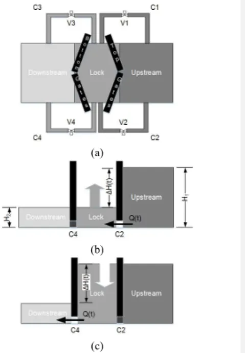
Fig. 1. Top (a) and side (b, c) views of the lock describing the filling (b) and draining (c) operations
Canal Lock Variable Speed Hydropower Turbine Design and Control
Jian Zhang
1*, Vlasios Leontidis
2, Antoine Dazin
2, Abdelmounaim Tounzi
1, Phillipe Delarue
1, Guy
Caignaert
2, Francis Piriou
1, Antoine Libaux
31 Lille Laboratory of Electrical Engineering and Power Electronics (L2EP), University of Lille, Bâtiment P2 59650, Villeneuve d'Ascq, France
2 Laboratoire de Mécanique des Fluides de Lille (LMFL), Ecole Nationale Supérieure d'Arts et Métiers, 8 Boulevard Luix XIV 59800, Lille, France
3 EDF Hydro-Engineering Centre Savoie Technolac, 73373, Le Bourget-du-Lac, France *[email protected]
Abstract: The design of a novel submerged hydraulic turbine for producing electricity by converting the available hydropower on canal locks during raising and lowering ships, but with the minimum overall impact on the facility, is being considered. The hydraulic head in such applications is low (few meters) and varies over time (from its maximum value down to zero) resulting in a low potential conversion of hydraulic head in electrical energy. The study involves the modification of the hydraulic transient system, the design and performance estimation of a hydraulic turbine. Based on the performance curves, a permanent magnet Vernier generator is designed. The models of hydraulic turbine and generator are added to the system model and simulations results of the whole system are presented.
1. Introduction
In “Hauts de France” region, more than 200 locks can be found all along a very dense network of rivers and canals allowing for goods and containers transportation. According to the rather flat landscape of the region, the locks are characterized by rather low water height differences between their upstream and downstream sides (generally around 3 m). Nevertheless, in a general context of energy saving, the potential energy recuperation during locks operation must be examined carefully.
A typical lock facility (Fig. 1) is characterized by a constant hydraulic head difference between upstream, H1, and downstream, H2, in the absence of any ship lock process (steady state), which is nearly independent of seasonal variations. The available gross head, ΔH(t), is quite small, in the order of few meters. When a boat arrives from the upstream direction two identical square guillotine valves (denoted as V1 and V2 on Fig. 1), positioned on the side channels (C1 and C2), are opened simultaneously and gradually in order the lock to be filled-up with water smoothly with a non-constant over time flow rate, Qi(t). By this way, it is assured that the flow of water is equally distributed in the two side channels and most important inside the lock minimum disturbances are being created in the free surface. During this operation the gross head starts to decrease and finally the level of water becomes equal in the two sides of the top gates which then open allowing the boat to enter the lock. Finally, the lock is being drained downstream with a similar procedure, through side channels C3 and C4. If a boat comes from the downstream direction then it is being captured inside the lock which is being filled-up until the water level reaches the upstream level.
The possibility of installing turbines in river locks has already been mentioned [1], but the process described is nearly impossible to be installed in an existing lock without major civil engineering modifications. However, a similar
work of designing and installing a hydro-turbine in an existing lock has not come to our knowledge.
On the contrary, a lot of work has been done over the last years to develop machines capable of producing energy from low and very low head hydro resources for different applications (e.g. river dams and irrigations channels) where
2 the head and/or flow are constant or minor changes are
being observed [2,3]. Nowadays, several types of turbines for very low head application are available in the market [4,5].
In conventional hydro power systems, a governor is used for controlling the turbine’s speed of rotation and producing the maximum energy. In the case under consideration, the turbine will be submerged, installed inside the side flow channel of the lock, where the water current will cause the blades to rotate. However, due to the variable water level the flow rate is never constant. Operating always at the best performance of the turbine, requires the rotation speed to follow the changes of the fluid velocity. This can be achieved by adopting a variable speed control system [6]. The idea behind the variable speed operation is to adjust the rotational speed for off-designed heads and/or discharge loads, which result in a reduced efficiency and could also lead to vibrations and cavitation problems [7,8]; thus, maximum efficiency power tracking at every operation point is being ensured [9,10]. For an axial propeller turbine, the overall efficiency is expected to be improved [9,11].
In addition, several studies have also focused on the design and control of systems intended for the conversion of wind or tidal energy, the principle of which is close to the problem of the conversion of canal lock hydropower into electrical energy [12-14].
The present paper is describing a project that aims in designing a hydro generator that can capture intermittent energy during the ship lock processes in the range of 30 to 60 kW and presenting the findings of the study. The overall goal is to develop an assembly consisting of a hydraulic machine and an energy conversion and controlling system, respecting constrains coming from the lock operation. Main characteristic of such facilities is the very low available hydraulic head which additionally varies with time, during operation, from its maximum value down to zero. Constraints that are being set are to minimize the effect on the operational time, minimize the intervention on the lock, and to be economically viable. One test case has been chosen as a basis for the project, but of course the models are not limited to that example.
In our previous works, the hydraulic machine [15] and the electrical system [16] were modelled separately and preliminary results were presented. A more detailed approach is now being followed, considering the influence of several parameters in their performance, including the interaction between the hydraulic and the electrical part of a turbine.
2. Hydraulic model of the lock
The whole system as presented on Fig. 1a is symmetrical between upstream and downstream, and between side channels. The side channels generally have a square cross section, are being made of concrete, and all are identical considering the dimensions, including the valves. Due to the symmetry, the system simulation is comprised of the lock, the upstream and two side channels with the corresponding valves.
It is obvious that one turbine can be installed in every side channel, but to retain the symmetry, which assures that the lock is being filled or drained as smoothly as possible, the cases of installing 2 or 4 turbines has been examined.
The results presented afterwards correspond to the operation of one turbine during one lock operation (filling or draining).
2.1. Hydraulic data
The initial available gross head between the upstream level, H1, and the downstream level, H2, is ΔHG = 3.03 m and the time duration to, to fill or drain the lock is around to = 480 s. For one year the total number of operations (fillings and drainages) is No = 7200. The total maximum potential theoretical energy, Eth, is:
𝐸ℎ=1
2𝜌𝑔𝑉 ∆𝐻 = 78.14 MJ (1) where ρ is the water density, g the acceleration of gravity and Vlock the volume of water incorporated to the lock during one filling sequence. In an annual basis, the maximum energy corresponds to:
𝐸 , = 𝑁 𝐸 ≈ 0.156 GWh/y (2)
This hydraulic energy can be converted to electrical by 2 turbines installed either on the upstream side (Fig. 1) during filling the lock or on the downstream side during emptying the facility. Thus, during a full operation cycle (fill and drain) the total theoretical available energy, and consequently the produced energy, can be doubled if 4 turbines are being installed.
2.2. Modelling of the lock transient operation Due to the absence of any flow data, first a dynamic model, using Simulink®, was developed for simulating the operation of the lock without the presence of any turbine and acquiring the evolution of the flow rate and the hydraulic head. The model is taking into consideration the pressure difference between the upstream, Pup, and the lock, Plock, the overall head losses, ΔPlosses, and the inertance, ΔPinert.
𝑃 − 𝑃 = ∆𝑃 + ∆𝑃 (3)
Upstream the hydraulic pressure is always constant, Eq. (4), whereas the pressure in the lock is changing over time, Eq. (5). Q is the total volume flow rate in the two side channels, whereas Qi is the flow in each side channel. The flow is being equally distributed in the two side channels. Slock is the section of the lock equal to the product of its length and width.
𝑃 = 𝜌𝑔𝐻 (4)
𝑃 (𝑡) = 𝜌𝑔𝐻 (𝑡) = 𝜌𝑔
𝑆 𝑄(𝑡)𝑑𝑡 (5)
Head losses occur in the channels and the valves. For the channels, the total losses can be described by Eq. (6), where kc is the total friction coefficient in the channels and Spipe is the cross section of the channel. The dimension of the cross section is 2.3 m x 2.3 m.
3 (a)
(b)
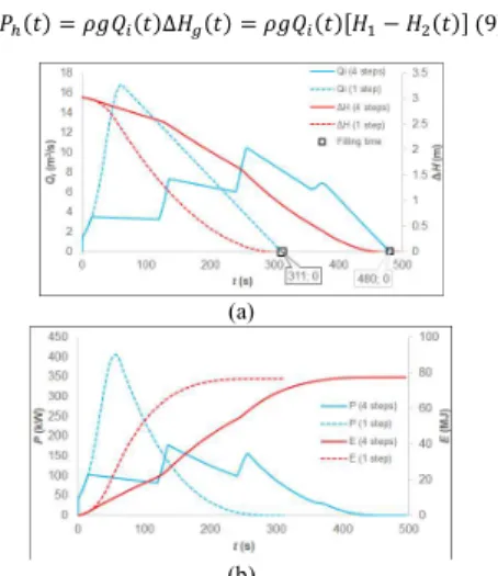
Fig. 2. Evolution of (a) the flow rate, Qi, and gross head, ΔΗ, and (b) the potential hydraulic power, P, and energy, E, under transient operation of the lock in one side flow channel with the modified valve operation and control (solid lines) and the initial law model (dash lines)
Fig. 3. Energy in the system for the default model (blue) and modified valve law model (red)
∆𝑃 (𝑡) =1 2𝑘 𝜌
𝑄 (𝑡)
𝑆 (6)
For the valve, the model of Eq. (7) was initially applied according to [16], where hv is the opening of the valve, changing 4 times every 2 min in equal intervals, from zero up to the maximum opening, hv,max, and τv is an exponential time constant. The valve opening between each step is linear over a period of Δτ = 20 s.
∆𝑃 (𝑡) = 381.6𝑒
ℎ ( ) ℎ, 𝜌 𝑄 (𝑡)
𝑆 (7)
Finally, the pressure difference in the water that is being required to cause a change in flow rate with time is given by Eq. (8), where Lpipe is the total length of the channels.
∆𝑃 (𝑡) = 𝜌𝐿
𝑆 𝑑𝑄(𝑡)
𝑑𝑡 (8)
The loss coefficient of the conduits can be estimated based on the head losses of the friction on the walls, the change of the direction in bends and the effects of the entrance and the exit of the channels [17]. A loss coefficient, kc = 4.087, is estimated.
The above system of equations is resolved to define the filling/draining time. The valve exponential time constant of Eq. (7) was fixed as the value for which the time is equal to to = 480 s and found to be τv = 7.17.
On Fig. 2, the evolution of the flow rate in one side channel is presented together with the available gross head and the dissipated hydraulic power, Ph. The dissipated energy, which is equal to the integration of the hydraulic power, has been also included in Fig. 2b and it can be observed that the total dissipated energy, Eq. (9), is perfectly equal to the maximum potential energy, defined before.
𝑃 (𝑡) = 𝜌𝑔𝑄 (𝑡)∆𝐻 (𝑡) = 𝜌𝑔𝑄 (𝑡)[𝐻 − 𝐻 (𝑡)] (9)
One of the main constrain, associated to the installation of the turbines, is to retain the duration of the transient operation close to the initial level (∼480 s), which will not be the case when introducing the turbines in the system. An additional source of losses will be added on the system resulting in an increase of the time cycle. The degree of the effect will depend on the selected machine and its design. A solution could be to modify the control law of the valves opening, for example force the valve to open in one step (continuously and linearly over time) and in a time interval of τv = 60 s. The results of the modified control and operation valve law are also presented on Fig. 2. The main characteristic of the proposed solution is that the same total dissipated energy, which is again perfectly equal with the maximum potential energy, is being acquired in a shorter time interval. The maximum flow rate is higher resulting in a shorter duration of the lock process and higher maximum hydraulic power. Despite the shorter operation time the losses in the flow channels are higher because of the higher bulk velocity (Fig. 3).
However, attention should be given in the possibility of disturbing the free surface, especially during the filling operation of the lock, because of the sudden increase of the flow rate. By increasing the required time for the valve to be completely opened in one step the potential effect on the boat stability can diminish, since the increment of the flow rate will be gentler and smooth, but the reduction of the total duration of the operation will not be significant.
The unsteadiness of the whole process is coming from the term of inertance, described by Eq. (8), which is not of great importance (Fig. 3). Thus, the degree of unsteadiness of the system is considerably low.
3. Hydraulic turbine design
First, a simple model of the turbine operation is being adopted and included on the dynamic model. Based on the preliminary results and by respecting specific restrictions the hydraulic machine is being selected and designed using a more detailed approach.
3.1. Hydraulic machine pre-design
A simple model for the turbine head drop, Eq. (10), based on the overall resistance coefficient of the hydraulic machine, kt, was introduced in the dynamic model. The resistance factor (kt = 138.76 kg/m7) was defined as the value for which the time for filling the lock is equal to around 480 s. The dissipated power in the machine can be calculated by Eq. (11).
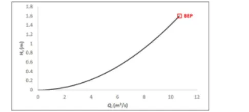
4 Fig. 5. Determination of the best efficient point (BEP)
Fig. 4. Duration of lock process (red) and energy recuperation (blue) for different values of the turbine overall resistance coefficient
∆𝑃 (𝑡) = 𝑘 𝑄 (𝑡) (10) 𝑃 (𝑡) = ∆𝑃 𝑄 (𝑡) (11)
A part of that energy will be transformed in electricity according to the type of machines (hydraulic and electric) and associated efficiencies. The level of the mechanical power can be modified by changing the imposed law of the valve, for example decreasing the time of the valve to fully open will result in more dissipated power. However, it must always be considered the impact of the flow rate evolution, which strongly depends on the valve control law, on the stability of the free surface in the lock and therefore on the stability of the boat. The turbine head, Ht, can be calculated:
𝐻 (𝑡) = 𝑃 (𝑡) 𝑄 (𝑡)𝜌𝑔 (12)
By integrating the turbine power, the total energy produced per turbine found to be Ei = 21.60 MJ, which represents 55% of the maximum potential energy. It has to be noted, that this analysis proposed as a first approach, is ignoring the minimum technical discharge of the turbine, which leads to a slight overestimation of the energy produced by the system. However, the total energy can be increased if the factor kt, is increased, but this will affect the duration of the whole operation. Different values of the resistance coefficient correspond to different designs of the turbine. It is also expected to change the pressure drop of the machine by modifying the rotational speed of the rotor.
Therefore, the simulation model can be used as an optimization tool for determining the correct value of kt to be used on a later step of the design procedure, for achieving the desired level of energy recuperation in compromise with the cycle duration. Fig. 4 summarizes the effects on the energy recuperation and the cycle duration. By increasing the factor kt, in other words increasing the turbine head drop, both the operation cycle and the power produced by the machine increase. The energy recuperation tends asymptotically towards to 100%, and further increase of the factor will result in very low energy gain.
3.2. Best efficiency point (BEP)
From the results of the simple modelling, a first estimation of the best efficient point (BEP) or design point of the turbine can be done for any value of the loss coefficient. The best efficient point is determined by the optimum flow rate, turbine head and rotational speed at
which the machine will have its maximum efficiency. On Fig. 5 the flow rate and head are being plotted for the case of kt = 138.76 kg/m7. The aim will be to design a machine which will have its best efficiency point for the maximum values of Qi and Ht. It has to be noted that the maximum value of Ht in Fig. 5 is around 1.6 m whereas the available water level difference at the beginning of the operation is 3 m. This difference is due to the energy dissipation in the pipes and valves of the hydraulic system. At this stage of the design, the efficiency at the best efficiency point is supposed to be ηBEP = 80%. It is expected that along the line of Fig. 5 the machine will always perform with its maximum efficiency.
In addition, the specific diameter, Ds, and speed, Ns, can be calculated. It is obvious that these parameters are not constant during the operation of the lock, because of the variable flow rate and head. Using the following equations, and the well-known Cordier diagram [18] the speed of rotation, N, is being calculated for the BEP.
𝐷 (𝑡) =𝐷[𝑔𝐻 (𝑡)]
.
𝑄 (𝑡) (13) 𝑁 (𝑡) = 𝑁 𝑄 (𝑡)
[𝑔𝐻 (𝑡)]. (14)
If the diameter of the machine is D = 2 m, slightly smaller than the width and the height of the side channels, it is found that N = 14 rpm. The calculated speed of rotation is quite small, making very difficult to design the electrical machine that will accompany the hydraulic part without gear box. A reason for that, except the very low head, can be the fact that Cordier diagram, which has been the statistical result of various commercial turbines, is not able to describe the operation of the specific application. Therefore, a higher rotational speed, at the BEP, will be assumed and fixed.
3.3. Hydraulic machine selection
The selection of the type of the hydraulic machine depends on many criteria, all of which are directly linked to the application under consideration. In the specific case, to predefine the machine type, several quantitative (available head, flow rate, rotational speed, cost) and qualitative factors (degree of intervention in the facility, portability, location) must be considered [19]. The main characteristic of the turbine under design is the very low head. It is a common practice in such applications to use axial reaction turbines and more precisely a propeller or Kaplan turbine.
5 (a)
(b)
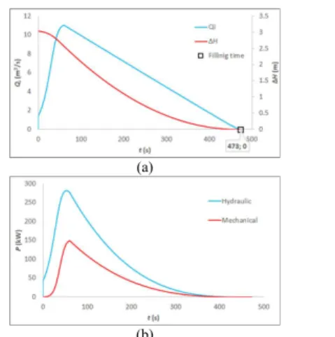
Fig. 6. Evolution of (a) the flow rate, Qi, and gross head, ΔH, and (b) the turbine power, P, with the detailed turbine model
As it can be understood, the design of the machine is based on two main parameters: an external diameter (in the case of an axial turbine) compatible with the cross-section dimensions of the existing channels, and the chosen value of kt. As mentioned before, the impeller speed of rotation can then be rather easily deduced using the Cordier diagram (which cannot be applied satisfactorily in the case under consideration) or a pre-defined fixed value can be used for the best efficient point. However, it will be clear afterwards that the final selection of the rotational speed will depend on the combination of the two systems: the hydraulic and the electrical. If the law used to model the turbine is validated, it can be observed that the use of an adequate variation of speed of rotation during the transient process can lead to correct machine efficiency during the whole operation. Controlling, thus, the speed with the electrical machine will result in controlling the flow evolution on the system.
Additionally, the specific machine is being required to be installed with the minimum intervention on the facility, meaning no civil works must be required, to be submerged mounted at the inlet or outlet of the side channels, but at the same time to be possible to be raised easily for purposes of maintenance and cleaning. And, of course, economical aspects must be considered in the early phase of the machines selection.
Based on the above criteria a simple non-regulated axial propeller was chosen to be designed for the case under consideration.
3.4. Detailed design of the turbine
3.4.1 Velocity triangles & design equations: A more comprehensive approach using the method of the velocity triangles and calculating the turbine hydraulic losses was applied [18,20] and the associated system of equations was included in the dynamic model. The simplest approach to the analysis and design of a hydraulic turbine is to assume that the flow conditions at the mean radius represent the flow at all radii. This two-dimensional analysis can provide a reasonable approximation of the actual flow, if the ratio of blade height to mean radius is small. The below assumptions were made:
Water enters the turbine in the axial direction. The axial component of the flow velocity is
constant.
At design point the flow velocity at the outlet is completely axial.
Mean radius is constant, and the radius of the tip and hub was taken equal to 1 m and 0.5 m, respectively.
16 guide vanes and 4 runner blades were considered.
The rotational speed at the BEP can be either determined based on the Cordier curve or fixed on a certain value. The flow through a reaction axial machine should accelerate, but this was not the case if the speed of rotation was calculated based on the Cordier diagram. On the contrary, a rotational speed could be found above which the flow starts to accelerate, and this occurred above 25 rpm. Additionally, restrictions coming from the design of the electrical machine must be taken into consideration in the final selection.
3.4.2 Transient process modelling: The rotational speed, N in rpm or ω in rad/s, will be changed during the lock process, which will lead to a better performance of the machine due to the variation of the flow rate and hydraulic head. At that phase of the study, the transient speed of rotation is following the similarity law of Eq. (15). Therefore, the turbines will always operate at the best efficient point resulting in high and constant efficiency during the lock process.
𝜔(𝑡) = 𝑄 (𝑡) 𝜔
𝑄 (15)
The detailed design of the turbines revealed a slight different filling time, comparing with the results of the simple turbine model which gave a time equal to 480 s. The evolution of the flow and gross head together with the corresponding evolution of the potential power and the mechanical power are given on Fig. 6.
The total energy produced is 18.51 MJ (or 47.38% of the potential energy). The amount calculated with the detailed model is less than the one predicted by the simple turbine model, because the losses in the machine are being considered, whereas in the simple model the efficiency was considered to be equal to 100%. The efficiency is being calculated by Eq. (16) and was found to be constant around 80%.
𝜂(𝑡) = (16)
3.4.3 Turbine characteristic curves: The characteristic curves (Fig. 7) of the hydraulic machine can be reproduced by performing simulations with constant flow rates, in the range of 1 to 15 m3/s, and linearly varying speed of rotation from 0 to 200 rpm. The rotational speed at design point was always 50 rpm, and the hub and tip radius 0.5 and 1 m,
6 Table 1 Turbine characteristic curves
𝐇𝐭(𝐐, 𝐍) = 𝐀𝟏𝐐𝐧+ 𝐁𝟏𝐐𝐍 + 𝐂𝟏𝐍𝟐 n A1 𝒎𝟑𝒏 𝟏 𝒌𝒈𝒏 B1 𝒎𝟒 𝒌𝒈. 𝒎𝒊𝒏 C1 𝒎 𝒎𝒊𝒏𝟐 1.763 0.0022 0.0054 -0.0006 𝝉(𝑸, 𝑵) = 𝑨𝟐𝑸𝟐+ 𝑩𝟐𝑸𝑵 A2 𝒌𝑵. 𝒎𝟕 𝒌𝒈𝟐 B2 𝒌𝑵. 𝒎𝟒 𝒌𝒈. 𝒎𝒊𝒏 0.5023 -0.0589 𝑷𝒎(𝑸, 𝑵) = 𝑨𝟑𝑸𝑵𝟐+ 𝑩𝟑𝑵𝑸𝟐 A3 𝒌𝑾. 𝒎𝟑 𝒌𝒈. 𝒎𝒊𝒏𝟐 B3 𝒌𝑾. 𝒎𝟔 𝒌𝒈𝟐. 𝒎𝒊𝒏 -0.0062 0.0526 (a) (b) (c) (d)
Fig. 7. Turbine characteristics curves for different flow rates: (a) power output, (b) turbine hydraulic head, (c) torque, (d) efficiency
Fig. 8. Maximum power tracking respectively. The best hydraulic efficiency of the turbine
obtained in Fig. 7d is consistent with the values obtained in recent numerical simulation concerning very low head turbines and a little bit higher than the efficiencies experimentally obtained in recent works [21-23].
At constant flow rate, the hydraulic head, the torque, and the power can be described as a function of the rotational speed:
𝐻 (𝑁) = 𝐴 𝑁 + 𝐵 𝑁 + 𝐶 (17) 𝜏(𝑁) = 𝐵 𝑁 + 𝐶 (18) 𝑃 (𝑁) = 𝐴 𝑁 + 𝐵 𝑁 (19)
where A, B and C are constants with the corresponding units. The constants depend on the flow rate, following perfectly a linear or power law. Therefore, the characteristic curves can
be expressed as a function of the speed of rotation and the flow rate (Table 1). Dividing the mechanical and the hydraulic power, an equation for the efficiency can also be produced.
𝜂(𝑄 , 𝑁) = 𝐴 𝑄 𝑁 + 𝐵 𝑁𝑄
𝜌𝑔(𝐴 𝑄 + 𝐵 𝑄 𝑁 + 𝐶 𝑄 𝑁 ) (20)
From Fig. 7a it is obvious that for every flow rate there is an optimum speed of rotation, Nopt, for which the turbine can produce the maximum power. This speed can be found by taking the maximum of the power output. The below equation can be used as a tool (Fig. 8) for tracking the maximum power for a specific flow rate and imposing the optimum rotational speed in Simulink model (instead of the law of similarity).
𝑑𝑃
𝑑𝑁= 0 ⇒ 𝑁 = −
𝐵
2𝐴 𝑄 (𝑡) (21)
Comparing with the results for which the law of similarity for the imposed rotational speed was used, there are slight differences in the filling time and the amount of energy being recuperated. The total energy produced was 18.61 MJ (or 47.64% of the potential energy).
4. Electromechanical conversion
The electromechanical conversion should transform the hydraulic power extracted by the turbine first to electrical power through the mechanical coupling between these two components. Then, the generated electrical energy
7 Fig. 9. Electrical system illustration
Fig. 10. Permanent magnet vernier machine is either delivered to the grid or to a local utility. As
introduced above, the turbine will be installed at the inlet or outlet of the side conduits in order to avoid any civil engineering modification and its rotation speed during the operation will not be constant. Therefore, whatever the chosen generator and the purpose of the conversion, static converters have to be used to generate a final voltage with constant amplitude and frequency. Thus, the architecture of the electromechanical conversion device is similar to those used in wind turbines or more specifically in tidal turbines at variable speed [24-27]. The main differences are relative to the generator to be used and to the most appropriate control for the application studied, due to the atypical character of flow of water as a function of time.
In the following sections, the overall scheme of the electromechanical conversion is first described. Then, the designed and sized electrical generator is introduced as well as the control principle adopted.
Finally, the models of the different mechanical and electrical parts are coupled and the whole system is simulated by applying the used control with the aim of extracting the maximum power using variable speed turbine-generator.
4.1. Electromechanical system
The whole electromechanical system is illustrated in Fig. 9. It constitutes of an electrical generator driven by the turbine and two static converters, i.e. a rectifier and an inverter for the converters 1 and 2 respectively.
In this system, the generator can be either immersed integrated with the turbine or out of water with its shaft mechanically coupled to the turbine through different devices. In our case, the first solution is chosen for reasons of compactness and simplifications of mechanical parts. Besides, in order to be able to control the energy flows and the different electrical quantities, the two static converters must be controllable and therefore, conventional PWM-controlled converters are used. As introduced previously, the flow rate in the channel is initially controlled by adjusting the opening of the valve. The extracted power of the turbine varies with flow rate and turbine rotational speed. The control of converter 1 (Fig. 9) leads then to controlling the torque created by the electrical machine and thus adjusting the turbine speed at the optimal operation points which depend on the turbine design parameters as explained in the last section. This process is therefore similar to Maximum Power Point Tracking (MPPT) in a wind turbine control [28].
The converter 2, placed between the DC bus and the electrical grid, leads to controlling the DC bus voltage at a constant value and the reactive power on the grid with sinusoidal current absorption. The control of the DC bus voltage leads to having the electrical grid power equal to the power generated by the electrical machine.
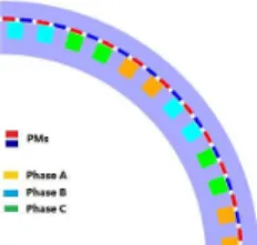
4.2. Permanent magnet Vernier generator Following the design of the turbine, the chosen generator has obviously to fulfil some specifications and constraints. Indeed, its rated speed has to be low in order to avoid any mechanical gearbox and its volume must be enough small in order to be housed in the available interior volume of the turbine. These two constraints cannot be satisfied at the same time by a classical direct driven Permanent Magnet Synchronous Machine (PMSM) as it requires large pole pair number to satisfy a rated low speed operation at standard frequency leading to a large diameter. Therefore, to reach a high torque at low speed operation while ensuring frequency of the electrical variables at standard value, a PM Vernier Generator Machine (PMVM) is designed, which has a simple structure comparing with classical PMSM [29,30]. The designed prototype is illustrated in Fig. 10. It is an inner stator outer rotor which provides the possibility to integrate the turbine blades into the latter.
In PMVM, the electromagnetic energy conversion is based on the interaction of armature magnetic field with the one of the rotating magnets which is modulated by the air gap permeance due to the open stator slots. Thus, to reach a continuous energy conversion at a synchronous speed, a special relationship among the rotor PM pole pair number pr, the stator winding pole pair number, ps, and the stator slots number, Ns, should be satisfied to obtain constant torque with low ripples.
𝑝 = 𝑁 ± 𝑝 (22)
Then, the synchronous speed, is linked to the stator frequency, by = /pr.
With the specifications of the studied application, an inner stator outer rotor prototype generator at 50 rpm and 36.6 Hz (pr = 44, ps = 4 and Ns = 48) has been analytically designed, optimized and verified by finite element analysis method [16].
8 Fig. 11. Generator side converter control structure
Fig. 12. Grid side converter control structure 5. System control and performance
To study the behaviour of the whole system, a simulation model of the electromechanical conversion system is built.
5.1. Permanent magnet Vernier generator model and control
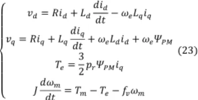
From the global point of view, the operation of the PMVM is quite similar to the PMSM. Therefore, its three-phase lumped parameter model is identical to the one of synchronous machine and can be expressed in dq rotating reference frame as follow [31]:
⎩ ⎪ ⎪ ⎨ ⎪ ⎪ ⎧ 𝑣 = 𝑅𝑖 + 𝐿 𝑑𝑖 𝑑𝑡− 𝜔 𝐿 𝑖 𝑣 = 𝑅𝑖 + 𝐿 𝑑𝑖 𝑑𝑡 + 𝜔 𝐿 𝑖 + 𝜔 𝛹 𝑇 =3 2𝑝 𝛹 𝑖 𝐽𝑑𝜔 𝑑𝑡 = 𝑇 − 𝑇 − 𝑓 𝜔 (23)
where v and i represent the voltage and current respectively, R is the winding resistance, ΨPM is the PM flux linkage, pr is the rotor pole pair number of the machine, ωe is the electrical rotational speed, ωm is the mechanical rotational speed, Tm is the load torque, Te is the generator torque and fv is the viscous damping, J is the inertia of the rotating parts in the system. J and fv are estimated values used in the simulation which will be modified in the prototype system to design the controller. Furthermore, as the magnets are rotor surface mounted, there is no reluctance saliency that can modulate the stator inductances, i.e. they are constant with respects to the rotor position. Hence, the dq-axes inductances are identical (Ld = Lq).
The values of the designed machine dq model parameters are identified from the numerical model of the optimized prototype and given in Appendix. This model is used to develop a control strategy based on classical vector current control (or field oriented control).
Fig. 11 shows the control scheme for the generator-side converter. As in the case of conventional surface mounted PMSM, the d-axis current reference is set to zero to minimize the copper losses of the generator [32]. The q-axis current reference is calculated by the speed loop controller. The input of the latter, i.e. speed reference, is obtained from the MPPT algorithm based on the measured or estimated flow rate.
5.2. Grid side model and control
The grid side model is like the generator one when RL filter model is chosen. The three phase voltages and currents of grid side can also be modelled in a dq reference frame as follows [33]:
𝑈 = 𝑟 𝑖 + 𝑙 − 𝜔 𝑙 𝑖 + 𝑈
𝑈 = 𝑟 𝑖 + 𝑙 + 𝜔 𝑙 𝑖 + 𝑈
(24) where the subscripts g and i denotes the grid and the inverter side, rf and lf are the grid side resistance and inductance, Udi and Uqi are the inverter side dq axis voltages, Udg and Uqg are the grid side dq axes voltages, idg and iqg are the grid side dq axes currents, ωg is the grid side frequency which can be determined by Phase Lock Loop (PLL method) [34]. Like in the generator side converter, the dq-axes currents and voltages are decoupled. This characteristic provides an effective mean for the independent control of the active and reactive powers of the system. The grid side active power, Pg, and reactive power, Qg, can be calculated by Eq. (25) [33]. Qg is controlled to zero to achieve unity power factor control. 𝑃 =3 2 𝑈 𝑖 + 𝑈 𝑖 𝑄 =3 2 𝑈 𝑖 − 𝑈 𝑖 (25)
Fig. 12 shows the grid side converter control structure. It contains two cascaded control loops. The inner loops control the grid currents or grid power and the outer loops control the DC-link voltage and the reactive power. In order to transfer the maximum available power to the grid from the DC-bus, the voltage of the DC-bus should be controlled at a constant reference value. In the inner current control loop, the dq-axes current references are calculated by Eq. (25). The outer loop gives out the active and reactive power references. The dq-axes voltages are obtained from the transformation of the measured grid side voltage.
9 Fig. 16. System illustrations with energy storage system (ESS)
Fig. 15. Grid side energy comparison for one operation (filling and draining water)
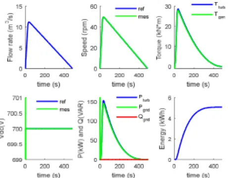
Fig. 13. Dynamic simulation results of one turbine for valve opened instantaneously
As already mentioned, the valves are controlled in four steps in a real typical lock and several scenarios are possible; either adding the turbine without changing the valve opening procedure, or letting the same procedure with different opening times or opening the valve in one step. The different processes of valve opening will be discussed in detail with respect to energy extracting.
The dynamic simulation equations described on the previous section are used to build an average model in Matlab/Simulink®. The grid side energy is compared for different operation valve process.
Fig. 13 shows the simulation results of one turbine when the valves are opened in one step. From the flow rate variation curve, it is known that the water in lock can be filled or drained in approximately 480 s. The measured rotational speed and the DC bus voltage follow their reference quite well. Grid side unity power factor is achieved as the reactive power is kept at zero. It indicates that the control parameters are tuned very well.
The cases when the valve is controlled to be opened in four steps with different opening times are also investigated. Fig. 14 shows the comparison of flow rate for different valve opening process. It can be seen that the peak flow rate becomes smaller when the valve is opened in four steps. The cycle time increases by about 50 s for opening step equal to 60 s and 120 s for a step of 120 s comparing to valve opened instantaneously. The peak flow rate in channel decreases when the valves are opened in longer time. As a reason of that, the draining or filling time increase. It reveals that the operation time for ship passing may increase one or two minutes once the turbine-generator system installed if the valve is opened in four steps. Furthermore, in terms of energy delivered to the grid, Fig. 15 illustrates the grid side energy comparison for the 3 cases. As expected, it shows that opening the valves in one step is the best solution as it can deliver more power to the grid side.
These results show that it is possible to convert the hydraulic energy of the canal lock filling or draining into electrical energy in an efficient way using a MPPT control. However, the energy delivered to the grid is intermittent and varies quickly. It is not suitable to inject the produced energy directly into the grid. Therefore, an energy storage system is needed to smooth the power profile.
6. Energy storage system
The canal lock available energy is strongly intermittent and can lead, in case of more powerful system, to non-negligible perturbation at the grid connection. To reduce potential grid side power oscillations, Energy Storage System (ESS) is adopted to smooth the power fluctuation.
The system topology with ESS is shown in Fig. 16. The latter is constituted of both batteries and supercapacitors. Indeed. battery has high energy density and low power density characteristics while supercapacitors have opposite characteristics. Therefore, they can compensate each other and can be of great interest in the case of the studied application as explained above. Flow battery type is adopted as it has flexible energy, high power density capability and long service life cycle. Furthermore, its self-discharge effect is very small [35].
Fig. 14. Flow rate comparison for different valve opening process
10 Fig. 17. VRB equivalent circuit model [36]
Fig. 19. ESS power flow control
P o w e r( kW )
6.1. Supercapacitors and DC–DC converters modelling
The supercapacitor is modelled as RC circuit. When charging, the voltage at its terminals can be deduced through the following relation:
𝑉 = 1
𝐶 ∫ 𝑖 𝑑𝑡 + 𝑖 𝑅 (26)
where isup is the supercapacitor current, Rsup is the supercapacitor resistance.
While connected to the buck DC–DC converter, a second equation must be applied to calculate the dynamics of the current isup:
𝐿𝑑𝑖
𝑑𝑡 + 𝑉 = 𝐷 𝑉 (27)
L is the buffer inductor inductance and Dcyc is the applied time-dependent duty cycle for the converter.
The above two equations can be used to build a dynamic average model for the coupling DC–DC converter/supercapacitors.
6.2. Battery modelling
The vanadium redox flow battery (VRB) technology is chosen and its model presented in this paper is mainly based on the reference [35,36].
Fig. 17 shows the flow battery equivalent circuit model where the stack current Istack and stack voltage Vstack represent the battery cell-stack internal current and electromotive force that permit to calculate the battery state of charge (SoC). The battery terminal voltage and current are expressed as Vbattery and Ibattery. The transient component associated with the electrode capacitance is modelled by Celetrode.
The losses are taken into account by the internal resistances Rreaction and Rresistive while the parasitic resistance Rfixed allows modeling the stack by-pass current. The power losses due to the circulation pump and the system controller are represented by the loss current Ipump. Finally, the switch on the parasitic branch is used to account for the battery standby mode. The parameter calculation process is detailed in [34].
6.3. Energy storage system power flow control In order to reduce the grid side power oscillation, it is assumed to control the grid side power as constant during the day. The ESS power (positive for charge mode) is set to
compensate the difference between the available power supply at DC bus PG and grid power demand as follows:
𝑃∗ = 𝑃 − 𝑃∗ (28)
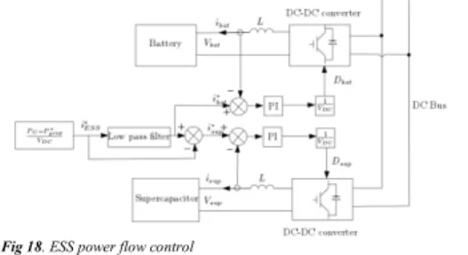
To be able to achieve a good control strategy in which the battery is mitigated of stresses, the high frequency part of the power should be sent to the supercapacitor and the low frequency part to the batteries. Then the power flow in battery and supercapacitor will be determined using low pass filter control strategy as shown in Fig. 18.
Based on the power references, the reference currents of battery and supercapacitor can be calculated as the DC bus voltage is controllable. The two current references will be then controlled by their corresponding PI controller. The outputs of the latter are the corresponding converter voltages which will be used to calculate the modulation duty cycles of the converters.
6.4. Simulation results with ESS
The assumption that there is only one operation of filling and draining water per hour in the day is made and two operations are simulated. The power flow in the system is shown in Fig. 19. The blue line shows the energy produced by the generator. The grid side power will be kept at the average level for one hour. At the beginning of each cycle, one part of the generator produced power will be transferred to grid. Then the rest power will be used to charge the battery and the supercapacitor. It can be seen that the supercapacitor charged faster than the battery. When the generator power is zero, the battery will be discharged to keep the grid side power as smooth as possible.
11 7. Conclusion
This paper presents the whole system of canal lock energy exploration for a facility located in the north of France with an available hydraulic head of 3 m by installing submerged turbines on the channels flow. Up to four turbines can be installed at each facility. All results presented above are for one turbine and during filling or draining the lock.
Hydraulic canal lock modelling and design of a non-regulated axial propeller turbine are detailed. For the electrical part, a permanent magnet Vernier (PMVM) is designed and optimized for this project. The variable generator rotational speed (0-50 rpm) is controlled depending on the estimated current flow (0-11 m3/s) to achieve maximum power tracking. The aim of grid side control is to keep the DC bus voltage constant. Therefore, the active power produced by the generator can be totally transferred to the grid side. The reactive power is controlled as zero. In addition, energy storage system is applied to control the power flow inside the system. Hence, the power can be smoothed for the grid side power integration.
The priority operation of canal lock facility is to facilitate the navigation of ships. Therefore, major civil engineer works, which will result in shutting down the facility, cannot be implemented to maximize the energy exploration. This limits the total harnessed energy. The hydraulic system can achieve efficiency about 47%. In the electrical part simulation, the generator core losses, generator mechanical losses and converter losses are not introduced in the model for simplicity in classical way. The electrical part efficiency is estimated about 90%. Therefore, the total energy per turbine transferred to the grid is approximately 40% of the available theoretical energy. The total recovered energy depends on the total number of turbines to be installed, and since only the cases of installing 2 or 4 machines is being considered (because it is important always to retain the symmetry of the canal lock and not to disturb the stability of the ships during filling/draining the lock) the total energy produced is around 62.5 MJ per operation (fill or drain) or 125 MJ in a full operation cycle. As this sum of energy is the additional benefit of ship passing, canal lock energy extracting should not be underestimated.
The present study was conducted to show the technical feasibility of converting available hydropower to electrical energy on canal locks during raising and lowering ships. It was carried out on a given lock, with a limited number of ships passing the lock per day, whose information is available. Moreover, it was conducted in a way that does not change the current operation of the lock. Therefore, a serious analysis of economic 'profitability' cannot be conducted only on the basis of the results presented. Apart from a pure sustainable development aspect, the economic study must consider the number of daily operations of the lock, its day-to-day working scale, the development of a forecasting strategy to optimize the energy recovered by operation etc. These points could be the subject of an extensive complementary work
.
The next step of the research project is to focus on a more detailed study of the channel power losses using numerical modelling method. Additionally, a scaled 1 kW
turbine-generator system has been developed for validating the developed dynamic model.
8. Acknowledgments
The project carried out in close collaboration by two research laboratories of Ecole Nationale Supérieure d'Arts et Métiers (ENSAM) and University of Lille, one specialized in turbomachinery (LMFL) and one in electromagnetic systems (L2EP), with the support of Electricité de France (EDF), the French electric utility company, and Voies Navigables de France (VNF), the French navigation authority responsible for the management of the majority of France's inland waterways network and the associated facilities. The work financially supported by the Region Hauts de France, EDF and VNF.
9. References
[1] Ship lock electrical energy generation, by N. Desy and P. Virta. (29 November 2005). US Patent 6,969,925B2 [2] Laghari, J.A., Mokhlis, H., Bakar, A.H.A., et al.: ‘A
comprehensive overview of new designs in the hydraulic, electrical equipment and controllers of mini hydropower plants making it cost effective technology’, Renew. Sust. Energ. Rev., 2013, 20, pp. 279-293 [3] Agglegate Group, 'Exploring the Viability of Low Head
Hydro in Colorado’s Existing Irrigation Infrastructure', Interim Report, 2010
[4] MJ2 Technologies, La Cavalerie, http://www.vlh-turbine.com/, accessed 5 January 2017
[5] Turbiwatt, Caudan, France, http://www.turbiwatt.com/, accessed 5 January 5, 2017
[6] Borkowski, D., Węgiel, T.: ‘Small hydropower plant with integrated turbine-generators working at variable speed’, IEEE Trans. Energ. Conv., 2013, 28, pp. 452-459
[7] Farell, C., Gulliver, J.: ‘Hydromechanics of variable speed turbines’, J. Energ. Eng., 1987, 113, pp. [8] Valavi, M., Nysveen, A.: ‘Variable-speed operation of
hydropower plants: Past, present, and future’, 22nd International Conference on Electrical Machines, Lausanne, Switzerland, 2016
[9] Borkowski, D.: ‘Maximum efficiency point tracking (MEPT) for variable speed small hydropower plant with neural network based estimation of turbine discharge’, IEEE Trans. Energ. Conver., 2017, 32, pp. 1090-1098 [10] Borghetti, A., Di Silvestro, M., Naldi, G., et al.:
‘Maximum efficiency point tracking for adjustable-speed small hydro power plant’, 16th PSCC, Glasgow, Scotland, 2008
[11] Lautier, P., O’Neil, C., Deschênes, C., et al.: ‘Variable speed operation of a new very low head hydro turbine with low environmental impact’, Electrical Power Conference, Montreal, Que., Canada, 2007
[12] Zhou, Z., Scuiller, F., Charpentier, J.F., et al.: ‘Power smoothing control in a grid-connected marine current turbine system for compensating swell effect’, IEEE Trans. Sustain. Energ., 2013, 4, pp. 816-826
[13] Barakat, M.R., Tala-Ighil, B., Chaoui, H., et al.: ‘Energetic macroscopic representation of a marine current turbine system with loss minimization control’, IEEE Trans. Sustain. Energ., 2018, 9, pp. 106-117
Commenté [P2]: Is it wise to mention that? Reviewers may ask us to wait for experimental measurements to submit the paper.
12 [14] Yin, M.H., Li, W.J., Chung, C.Y., et al.: ‘Optimal
torque control based on effective tracking range for maximum power point tracking of wind turbines under varying wind conditions’, IET Renewable Power Generation, March 2017, vol 11, pp. 501-510 [15] Leontidis, V., Zhang, J., Caignaert, G., et al.: ‘Lock
hydro-electrical power generation feasibility study’, 19th International Seminar on Hydropower Plants, Vienna, Austria, 2016
[16] Zhang, J., Tounzi, A., Delarue, P., et el.: ‘Quantitative design of a high performance permanent magnet Vernier generator, IEEE Trans. Magn., 2017, 53 [17] Idel’cik, I.E.: ‘Memento des pertes de charge’, Eyrolles,
Paris, 1969
[18] Dixon, S.L., Hall, C.A.: ‘Fluid Mechanics and Thermodynamics of Turbomachinery’, Elsevier, 2010 [19] Elbatran, A.H., Yaakob, O.B., Ahmed, Y.M., et al.:
‘Operation, performance and economic analysis of low head micro-hydropower turbines for rural and remote areas: A review’, Ren. Sust. Energ., 2015, 43, pp. 40-50 [20] Albuquerque, R.B.F., Manzanares-Filho, N., Oliveira, W.: ‘Conceptual optimization of axial-flow hydraulic turbines with non-free vortex design’, P. I. Mech. Eng. A – J. Pow., 2007, 221, pp. 713-725
[21] Samora, I., Hasmatuchi, V., Münch-Alligne, C., et al.: ‘Experimental characterization of a five blade tubular propeller turbine for pipe inline installation’, Renew. Energ., 2016, 95, pp. 356-366
[22] Jawahar, C.P., Michael, P.A: ‘A review on turbines for micro hydro power plant’, Renew. Sust. Energ. Rev., 2017, 72, pp. 882-887
[23] Singh, P., Nestmann, F.: ‘Experimental optimization of a free vortex propeller runner for micro hydro application’, Exp. Therm. Fluid. Sci., 2009, 33, pp. 991-1002
[24] Frid, C., Andonegi, E., Depestele, J., et al.: ‘The environmental interactions of tidal and wave energy generation devices’, Env. Imp. Assess., 2012, 32, pp. 133-139
[25] Whitby, B., Ugalde-Loo, C.E.: ‘Performance of pitch and stall regulated tidal stream turbines’, IEEE Trans. Sustain. Energ., 2014, 5, pp. 64-72
[26] Uihlein, A., Magagna, D.: ‘Wave and tidal current energy – A review of the current state of research beyond technology’, Renew. Sust. Energ. Rev., 2016, 58, pp. 1070-1081
[27] Zhang, J., Moreau, L., Machmoum, M., et al.: ‘State of the art in tidal current energy extracting technologies’, International Conference on Green Energy ICGE 2014, Sfax, 2014
[28] Cui, Z., Song, L., Li, S.: ‘Maximum power point tracking strategy for a new wind power system and its design details’, IEEE Trans. Energ. Conver., 2017, 32, pp. 1063-1071
[29] Li, D., Qu, R., Li, J., et al.: ‘Analysis of torque capability and quality in Vernier permanent-magnet machines’, IEEE Trans. Ind. Appl., 2016, 52, pp. 125-135
[30] Toba, A., Lipo, T.A.; ‘Generic torque-maximizing design methodology of surface permanent-magnet Vernier machine’, IEEE Trans. Ind. Appl., 2000, 36, pp. 1539-1546
[31] Li, J.: Design, ‘Analysis and control of permanent-magnet vernier machines’, PhD thesis, University of Hong Kong, Pokfulam, Hong Kong SAR, 2012 [32] Sun, T., Wang, J., Chen, X.: ‘Maximum torque per
ampere (MTPA) control for interior permanent magnet synchronous machine drives based on virtual signal injection’, IEEE Trans. Power Electr., 2015, 30, pp. 5036-5045
[33] Zhang, J.: ‘Optimization design and control strategies of a double stator permanent magnet generator for tidal current energy application’, Phd thesis, Université de Nantes, 2015
[34] Das P.P., Chattopadhayay, S., Palmal, M.: ‘A d–q voltage droop control method with dynamically phase-shifted phase-locked loop for inverter paralleling without any communication between individual inverters’, IEEE Trans. Ind. Electr., 2017, 64, pp. 4591-4600
[35] Li, W., Joós, G., Bélanger, J.: ‘Real-time simulation of a wind turbine generator coupled with a battery supercapacitor energy storage system’, IEEE Trans. Ind. Elect., 2010, 57, pp.1137-1145
[36] Zhou, Z.: ‘Modelling and power control of a marine current turbine system with energy storage devices’, PhD thesis, Université de Bretagne Occidentale, 2014 10. Appendix
System parameters list:
dq-axes inductances 4.2 mH
Flux 1.41 Wb
System total inertia 1300 kg.m2
Pole pair number 44
Generator stator resistance 0.1 Ω
DC-bus capacitor 2 mF
DC-bus voltage 700 V
Grid-side resistance 0.01 Ω
Grid-side inductance 1 mH