HAL Id: dumas-00907303
https://dumas.ccsd.cnrs.fr/dumas-00907303
Submitted on 21 Nov 2013HAL is a multi-disciplinary open access
archive for the deposit and dissemination of sci-entific research documents, whether they are pub-lished or not. The documents may come from teaching and research institutions in France or abroad, or from public or private research centers.
L’archive ouverte pluridisciplinaire HAL, est destinée au dépôt et à la diffusion de documents scientifiques de niveau recherche, publiés ou non, émanant des établissements d’enseignement et de recherche français ou étrangers, des laboratoires publics ou privés.
Effects of hydro-morphological restoration of Dutch
lowland streams on macrophytes : relations between fine
scale physical features and aquatic plants communities
Claire Poupin
To cite this version:
Claire Poupin. Effects of hydro-morphological restoration of Dutch lowland streams on macrophytes : relations between fine scale physical features and aquatic plants communities. Agricultural sciences. 2013. �dumas-00907303�
- MEMOIRE DE FIN D’ETUDES -
Diplôme d’Ingénieur de l’Institut Supérieur des Sciences Agronomiques, Agroalimentaires, Horticoles et du Paysage
Année universitaire : 2012 – 2013
Spécialité : Génie de l’environnement
Option : Préservation et aménagement des milieux – Ecologie quantitative
Effects of hydro-morphological restoration of Dutch lowland streams on macrophytes: relations between fine scale physical
features and aquatic plants communities
Par : Claire POUPIN
Volet à renseigner par l’enseignant responsable de l’option/spécialisation Bon pour dépôt (version définitive)
Date : / / Signature : Autorisation de diffusion : Oui Non
Devant le jury : Soutenu à Rennes, le : 13 septembre 2013
Sous la présidence de : Jacques Haury
Maître de stage : Rob Fraaije Enseignant référent : Ivan Bernez Autres membres du jury: Marie Nevoux
"Les analyses et les conclusions de ce travail d'étudiant n'engagent que la responsabilité de son auteur et non celle d’AGROCAMPUS OUEST" Ecology and Biodiversity group
Utrecht University
Padualaan 8 3584 CH Utrecht, Netherlands
AGROCAMPUS OUEST, CFR Angers Institut National d’Horticulture et de Paysage
2 rue André Le Nôtre 49045 Angers CEDEX
Fiche de confidentialité et de diffusion du mémoire
Cadre lié à la confidentialité :
Aucune confidentialité ne sera prise en compte si la durée n’en est pas précisée.
Préciser les limites de la confidentialité (2) :
Confidentialité absolue : oui non
(ni consultation, ni prêt)
Si oui 1 an 5 ans 10 ans
Le maître de stage(4),
Cadre lié à la diffusion du mémoire :
A l’issue de la période de confidentialité et/ou si le mémoire est validé diffusable sur la page de couverture, il sera diffusé sur les bases de données documentaires nationales et internationales selon les règles définies ci-dessous :
Diffusion de la version numérique du mémoire : oui non
Référence bibliographique diffusable(3) : oui non
Résumé diffusable : oui non
Mémoire papier consultable sur place : oui non
Reproduction autorisée du mémoire : oui non
Prêt autorisé du mémoire papier : oui non
……….
Diffusion de la version numérique du résumé : oui non
Si oui, l’auteur(1) complète l’autorisation suivante :
Je soussigné(e) , propriétaire des droits de reproduction dudit résumé, autorise toutes les sources bibliographiques à le signaler et le publier.
Date : Signature :
Rennes/Angers, le
L’auteur(1), L’enseignant référent
ou son représentant
(1) auteur = étudiant qui réalise son mémoire de fin d’études
(2) L’administration, les enseignants et les différents services de documentation d’AGROCAMPUS OUEST s’engagent à respecter cette confidentialité. (3) La référence bibliographique (= Nom de l’auteur, titre du mémoire, année de soutenance, diplôme, spécialité et spécialisation/Option)) sera signalée dans les bases de données documentaires sans le résumé.
(4) Signature et cachet de l’organisme
ACKOWLEDGEMENTS
My special thoughts go to:
- Rob Fraaije, my supervisor: for bringing “stroop waffels” and coffee during the fieldwork
and being really involved in this research
- Ivan Bernez, my adviser: for always answering my emails and for his relevant advice; - Anais: for her priceless help with R; I would still be googling R error messages without her; - Fotis, Helena, Maria and Miquel: for maintaining food supply at home and cooking for me during the writing, and also for their cheering company when breaks were necessary;
- Megan: for attending my presentation rehearsal trying to understand what it was about but still listening until the end of it;
And finally, to all my good friends (that will recognise themselves if they ever read this report) for telling me about their holidays in sunny places while I was writing these acknowledgements.
CONTENTS
INTRODUCTION ... 1
MATERIALS AND METHODS ... 6
RESULTS ... 10
I) Comparison of restored and unrestored reaches ... 10
A) Physiochemical parameters ... 10
B) Plants data ... 11
1) Species diversity ... 11
2) Growth forms diversity ... 12
II) Relations between macrophyte communities and physical features ... 13
A) Water depth and distance to the bank ... 13
1) Species diversity ... 13
2) Growth forms diversity ... 15
B) Influence of meanders ... 18
1) Comparison between bends and straight parts ... 18
2) Comparison of inner bends, outer bends and straight edges ... 19
DISCUSSION ... 20
I) A contrasted response of species diversity between stream channel and edges ... 20
II) Differences in response according to growth forms ... 22
III) A relative influence of meanders ... 23
CONCLUSION ... 26
FIGURES
Figure 1 : Study design. ... 6
Figure 2 : Relations between coverage (1), species richness (2) and Shannon diversity (3) and depth (a) and distance to the bank (b). ... 13
Figure 3 : (a) Relations between depth and distance to the bank; (b) Normal QQ-plot of GLM residuals; (c) Normal QQ-plot of lm residuals. ... 14
Figure 4 : Relations between the coverage of a) amphibious species, b) emergent species and c) submerged species with water depth. ... 15
Figure 5 : Relations between the coverage of a) amphibious species, b) emergent species and c) submerged species with distance to the bank. ... 16
Figure 6 : Relations between 1) growth forms richness and 2) growth form diversity and a) depth and b) distance to the banks ... 16
Figure 7 : Growth forms richness in relation to a) depth and b) distance ... 17
Figure 8 : Comparison of a) flow velocity variation, b) species richness and c) Shannon diversity between bends (B) and straight parts (S)... 18
Figure 9 : Relationships between a) species richness and b) Shannon diversity and flow velocity variation ... 18
Figure 10 : KA after restoration ... 20
Figure 11 : Drawing illustrating the interaction between depth and distance to the bank on plant growth. ... 21
TABLES
Table 1 : Summary of number of plots per stream. ... 7
Table 2: Summary of physiochemical variables. ... 7
Table 3 : Presentation of the growth forms observed on the field ... 8
Table 4 : Summary of plant communities’ variables. ... 9
Table 5 : Physiochemical parameters of each stream ... 10
Table 6 : Plant parameters of each stream ... 11
Table 7: Growth forms’ parameters ... 12
Table 8 : Results of the regressions on species richness and Shannon diversity. ... 14
Table 9 : Correlation coefficients between coverage and depth, and coverage and distance to the bank. ... 15
Table 10 : Correlation coefficients between emergent species’ coverage and depth and distance to the bank. ... 16
Table 11 : Correlation coefficients between growth forms richness and diversity and depth and distance to the bank. ... 17
Table 12 : Comparison of physical features, plant parameters and growth forms frequencies between inner bends, outer bends and straight edges ... 19
p. 1
INTRODUCTION
Historical management of watercourses
“God created the world, but the Dutch made the Netherlands”. This old saying refers to the fact that the Dutch literally built their country over what originally was a low-lying delta mainly made of sediments from the North Sea and the Rhine and Meuse rivers. Indeed, centuries of water management converted this land, of which more than the half was covered by wetlands (including wide and unbridled river valleys, bogs, freshwater and coastal marshes; (Nienhuis et al., 2002b) into the well-known current Dutch landscape.
As mentioned by Nienhuis et al. (2002a), although humans have grown arable crops in the Netherlands for about 7000 years, the first impacts on watercourses only arose around 1000 years ago. Until then, the population remained on the elevated lands, naturally protected from floods, and cleared forested areas to turn them into suitable land for agriculture. So, back to then, rivers were barely altered, even though the Romans had locally modified watercourses by digging canals (Berendsen, 2005).
The first significant water management measures date back to the 11th century, when men
eventually went down the elevated lands, started to take over the fertile floodplains to grow
crops, and began building flood defence levees. But it’s only in the late 14th century that
human intervention on rivers began more intensive and that channelisation became common, in order to enable navigation, but also for other purposes such as water resource control and
flood management. The last period of major watercourses’ alteration spreads from the early
1900’s until the 1970’s, when many dams were built for electricity production and drinking water supply all across Europe (and therefore impacting downstream reaches of impounded rivers including Rhine and Meuse), while more and more streams kept on being channelised.
Anthropogenic impacts on streams
This large scale channelisation reached such an extent that, nowadays, 96% of Dutch streams are directly impacted by human activities (Verdonschot & Nijboer, 2002), which makes them one of the most vulnerable ecosystems in this country.
p. 2
Indeed, channelisation, consisting in any activity that straightens, broadens, cuts off or diverts a stream channel, radically impacts stream systems (Wasson et al., 1995 and references herein). First, morphology of channelised watercourses is deeply modified since both lateral and longitudinal profiles of the streambed are reshaped: channelisation usually results in an oversized stream bed (wider and deeper cross-section) and a shorter and steeper lengthwise section (Baattrup-Pedersen et al., 2005). These alterations lead to modified hydrological dynamics of the streams: flow velocities decrease during base flows in summer and increase during peak flows in winter (Verdonschot & Nijboer, 2002). On the one hand, very low flow velocity can lead to an increase in turbidity and algae development, and a decrease of dissolved oxygen that can in extreme conditions cause fish to die and plants to disappear (Verdonschot et al., 2012). On the other hand, the winter faster flows cause flooding events in the downstream areas and increase the erosive character of channelised streams, whose beds are then subjected to scouring and incision (Nienhuis et al., 2002 a,b). The consequent lowering of the stream bed then affects lateral connectivity with adjacent lands (Rambaud et al., 2009) and leads to a reduction of the water table in the riparian area. As a result, floodplains suffer from more frequent drought events, affecting the soil moisture gradient. Furthermore, modifications due to channelisation induce a loss of physical heterogeneity within the stream bed: its dimensions are standardised and riffles/pools sequences as well as meanders disappear, thus depleting the range of current velocities (Amoros & Bornette, 2002; Baattrup-Pedersen et al., 2005). Moreover, the homogenisation can sometimes even be accentuated by maintenance measures (like dredging) that frequently go along with channelisation (Baattrup-Pedersen et al., 2002).
Concurrently to these changes in streams’ hydro-morphology, the development of
intensive agriculture in the second half of the 20th century and thereby the increasing use of
fertilizers led to the eutrophication of water (both surface and groundwater), thus favouring very competitive species and reducing species richness (James et al., 2005). In addition to that, the increasing use of water for industrial purposes and the increase of demography in the same period led to a higher discharge of wastes in watercourses that also impacted the water quality.
Thus, the combination of physical and chemical alteration of stream led to a manifest simplification of instream habitats and shifts in aquatic biota (Arts, 2002; Kristensen et al., 2012).
p. 3
A need for innovative restoration measuresOver the past decades, concern about the degradation of streams led the public authorities to undertake measures in order to improve stream habitat quality. As a result, water quality of many European streams has improved during the past two decades (Pedersen et al., 2006), and many restoration projects were carried out to improve stream physical conditions. In this report, the word “restoration” refers to any measure that directs an ecosystem development towards a target ecosystem (Burmeier et al., 2011).
In the Netherlands, the first stream restoration projects date from the 60’s, but it really
became common from the 90’s onward. Unfortunately, in many cases, the expected improvement of ecological quality in restored streams is not reached (Waterschap Veluwe,
2009; Kristensen et al., 2012). Indeed, morphological reshaping didn’t lead to a more natural
hydrology: stream beds remained too wide and deep, thus maintaining very low current velocities in summer and impeding floodplain inundation (Verdonschot & Nijboer, 2002). Thus, neither the improvement of water quality nor previous restoration measures had the expected consequences on stream biota, and the ecological quality and biodiversity of lowland streams has even kept on declining in the meanwhile (Kristensen et al., 2012). Moreover, in 2000, the Water Framework Directive set the objective of good ecological status for water within the EU. Member states thus have a legal obligation to reach this objective. In the event that a member state would not reach it on time, it would be subject to a monetary fine.
As a consequence of this general lack of ecological improvement, and in order to meet the requirements set by the WFD, Dutch Waterboards decided to try out innovative restoration measures, which are aimed to balance hydro-morphological dynamics in order to
improve stream functioning. This new restoration project (called ‘Beekdalbreed
hermeanderen’) came up in 2010 and encompasses reshaping the stream bed to make it less
wide and deep, flattening the banks’ slope and creating meanders. Special attention is given to hydraulic connections between the stream and the floodplain in order to enable floodplain inundation and thus restore a moisture gradient in the riparian zone. These measures are expected to reestablish more natural flow velocities and a higher spatio-temporal heterogeneity which may increase biodiversity in the whole stream system, including the floodplain (Waterschap Veluwe, 2009).
Research teams from Wageningen and Utrecht universities, in collaboration with Dutch waterboards, seized the opportunity of this new restoration scheme to get a better
p. 4
insight on restoration impact on plants, macroinvertebrates and hydro-morphology within the whole stream ecosystem. The present study, carried out within the ‘Ecology and Biodiversity’ team of Utrecht University, focuses exclusively on macrophytes’ response to restoration; therefore, the question of riparian zone is not addressed in this report.
Why studying macrophytes?
As a result of the aforementioned anthropogenic alterations on aquatic systems, 90% of macrophyte habitats have disappeared in the Netherlands (Nienhuis et al., 2002a), and, as observed in most of western Europe lowland streams, the remnant aquatic plants communities have suffer from species diversity decline and homogenisation (Baattrup-Pedersen et al., 2003).
And yet, macrophytes, (defined as large aquatic plants that are not planktonic or filamentous algae; Bornette & Puijalon, 2011) play a key role in stream ecosystems. First, as primary producers, they provide food for many faunistic groups including bird, fishes and invertebrates (Riis & Biggs, 2003). Moreover, macrophytes constitute an important habitat within the stream since they supply shelter and substrate for epiphytic algae, invertebrates, fishes and frogs (Bornette & Puijalon, 2011). Furthermore, they strongly influence the hydrology of the streams, since they can raise the water level and induce flow velocity variation (the flow is reduced within the macrophytes stands and accelerates around them; Sand-Jensen & Mebus, 1996). These flow variations impact on sediment dynamics: slow flow enables sedimentation whereas fast flow favours suspension (Pedersen et al., 2006). Therefore, macrophytes can significantly increase stream habitat heterogeneity.
Because of the different functions they have within the stream system, changes in macrophyte communities can have significant consequences on the stream biota (Franklin et
al., 2008). Thus, macrophyte communities’ recovery might be a key stage towards a higher
stream’s biodiversity and the good ecological status of aquatic ecosystems required by the WFD.
p. 5
Aim of the studyThe first goal of this study is to evaluate the short-term effects of the above mentioned restoration measures on macrophytes communities and their habitat. Despite the increasing number of restoration operations, only little is known about macrophyte response, since most studies have so far focused on fauna, or on riparian vegetation (Lorenz et al., 2012). To do so, physical features and plants parameters were compared between restored and unrestored reaches. As a result of potentially more heterogeneous habitats, restored stretches are expected to feature higher plant diversity than the unrestored ones.
The further goal of this study is to identify relationships between fine scale stream physical features and macrophytes communities in order to assess which hydro-morphological modifications had the most significant influence on aquatic plants. Indeed, understanding these relations is essential to carry out successful restoration operations. And yet, although the main drivers of macrophytes abundance and distribution are known (Lacoul & Freedman, 2006; Bornette & Puijalon, 2011), quantitative knowledge is still lacking, thus preventing researchers and managers from predicting the outcome of restoration. In this part, we focused on the hydromorphological factors that were deliberately modified during the above mentioned restoration measures, that are water depth, distance to the bank, flow velocity variation and meanders. Depth and distance to the banks are expected to be negatively linked to plant diversity because of light limitation in deeper water (Caffrey et al., 2007) and the importance of bank plants for instream vegetation colonisation (Riis et al., 2001). On the contrary, a higher physical heterogeneity (meanders, higher flow velocity variation) is expected to be positively related to plant diversity since it may provide more ecological niches for macrophytic species (Palmer et al., 2010).
p. 6
MATERIALS AND METHODS Study sites and design:
The study was carried out on three lowland streams located in the South-East quarter of the Netherlands: Hagmolenbeek, Kleine Aa and Luntersche beek, henceforth referred as HM, KA and LB (map in appendix I). Those three streams were respectively restored in June 2010, October 2011 and July 2011. Lowland streams, mostly fed by rainwater, are common in the flat areas of Western European plain and are characterised by a low slope (comprised between zero to five per mil) and sandy soils (Verdonschot & Nijboer, 2002).
As there was no data available on plant communities before restoration, the study design is based on a space-for-time substitution. On each stream, 9 homogeneous sections in terms of water depth and bed width were selected: 3 located in an unrestored reach, 6 in a restored one. Among the 6 restored sections, 3 were placed in straight stretches, and the 3 others in bends (figure 1). 5 transects made of 25 cm * 25 cm plots were regularly spread within each section. The first and the last plots of each transects were placed so that the beginning of the bank was included. Plots were classified in three categories: riparian plots (the ones including
the beginning of the bank), edge plots (the ones present in the first 5th of stream width), and
channel plots.
p. 7
The number of plots per stream and restored (R) and unrestored (U) sections are presented in the table X:
Table 1 : Summary of number of plots per stream, separating restored and unrestored sections.
HM KA LB All streams All
streams
R U R U R U R U
Number of plots 293 504 931 595 755 374 1979 1473 3452
Physiochemical parameters:
In the centre of each 25cm * 25 cm plot, water depth and distance to the bank were measured with a GPS (in May and June 2013). The dominant substrate type in the first 10 cm
of soil was also recorded per plot and categorised as stone (>60 mm diameter), gravel (3–60
mm), sand (0.25–3 mm), silt(<0.25 mm), hard clay or peat. The substrate data was then
pooled per section and the percentage of each substrate type was then calculated [number of plots with substrate “a” / total number of plots of the section * 100] at the section level.
Flow velocity was measured in May 2013 in three plots per transect: one in the channel, and the two others in each edge (as previously defined). Flow velocity variation was then estimated per transect by calculating the coefficient of variance (standard deviation / mean).
In April and May 2013, available phosphorous (Olsen method) and nitrogen (KCL method) for the growing season were measured at the section level. Substrate and nutrient availability were recorded in order to ensure they were not too different between the different streams, and were not used as explanatory variables in the regressions, since the focus of the study is on the physical features that were modified during the restoration (depth, width, flow velocity variation). Physiochemical variables are summarised in the table 2.
Table 2: Summary of physiochemical variables.
Variable
Scale Depth Distance to
the bank Width Substrate
Flow velocity Flow velocity variation Available P and N Plots x x x x x Transects x x x Section x
p. 8
Vegetation survey:
Macrophytes survey was carried out from mid-June to mid-July 2013 in the same 25 cm * 25 cm plots used to measure the water depth and distance to the bank. Their abundance was expressed as a percentage of coverage. The survey was undertaken by wading through the stream and using a “viewing tube”. Plants were identified on site to the species level except the ones that required special features non visible at the time of the survey (i.e. Callitriche
sp.). In this case, they were identified at the genus level. Plants that were not identified on
site were sampled and brought back to the laboratory for further identification.
In the present study, plant diversity was expressed as the number of species (species richness), and Shannon diversity index (explanation Shannon), and were calculated for each plot and also at the transect level in restored sections. Shannon diversity index is calculated using the following formula:
H′= − ∑ ( PiP ∗ log2 PiP )
� �=1
with:
The index ranges from 0 to log2(S). It takes into account the coverage of the different species in a plot: a low value reflects the dominance of one species (“low diversity”) whereas
a high value indicates the co-dominance of several species (“higher diversity”).
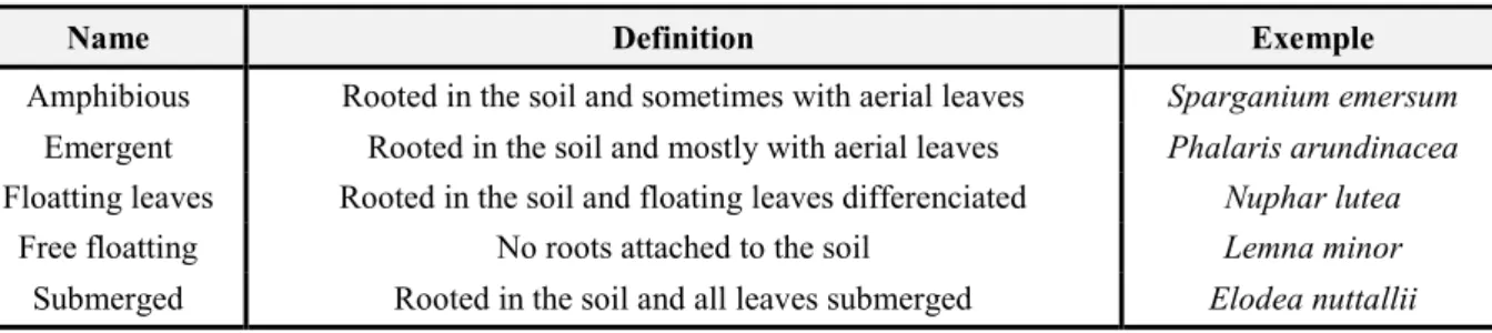
The analysis of growth forms can give valuable information on habitat structure and on the functional diversity on macrophytes communities since they are characterised by different morphologies and niches (Cadotte et al., 2011).Therefore, species were classified according to their observed growth form as either amphibious, emergent, floating leaves, free floating and submerged. The definitions of each growth forms are presented in the table 3.
Table 3 : Presentation of the growth forms observed on the field (adapted to the observed flora from Daniel et al., 2006).
Name Definition Exemple
Amphibious Rooted in the soil and sometimes with aerial leaves Sparganium emersum
Emergent Rooted in the soil and mostly with aerial leaves Phalaris arundinacea
Floatting leaves Rooted in the soil and floating leaves differenciated Nuphar lutea
Free floatting No roots attached to the soil Lemna minor
Submerged Rooted in the soil and all leaves submerged Elodea nuttallii
- S = Species richness
- Pi = Coverage of species i in the plot - P = Total coverage in the plot
p. 9
The coverage of each growth form was calculated per plot by adding the coverages of the species belonging to the same growth form. The relative frequency of each growth form was calculated per plot as following: [number of species of growth form “a” / total number of
species * 100] and is hereafter referred to as “frequency”. The functional diversity was
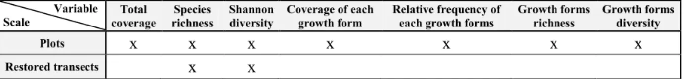
expressed as the number of growth forms (growth form richness) and growth form Shannon diversity and both were also calculated for each plot. The variables calculated from data plants are summarised in the table 4.
Table 4 : Summary of plant communities’ variables. Variable Scale Total coverage Species richness Shannon diversity Coverage of each growth form Relative frequency of each growth forms
Growth forms richness Growth forms diversity Plots x x x x x x x Restored transects x x Data analysis :
First, PCA were performed on species and growth forms data in order to visualize them and to identify general patterns. In order to diminish the influence of rare plants, only the ones that were present in more than 1% of the plots (i.e. in at least 35 out of the 3425 plots) were selected (appendix II-b).
For statistical analysis, variables’ distributions were graphically assessed with normal
qq-plots. None of the variables were normally distributed so classical transformations (square root (x); ln(x) + 1) were applied. As they didn’t lead to normal distribution, comparisons were performed using non-parametric tests, i.e. Wilcoxon test for simple comparisons and Kruskal-Wallis test for multiple comparisons.
Before regressions, correlation was tested between explanatory variables with Spearman correlation test to exclude strongly redundant variables (r² > 0.8 and P < 0.05; Ernoult et al., 2013). Relationships between species richness and depth and distance to the banks were tested using generalised linear models (GLM) with a Poisson family distribution error. The fit of the model was expressed by the percentage of deviance explained by the GLM [i.e. (null deviance - residual deviance) / null deviance * 100)]. Relationships between Shannon diversity and the same explanatory variables were tested with linear regressions. The fit of the model was expressed as the adjusted R². For both GLM and linear regression, the relevance of the models was assessed by checking the distribution of models’ residuals (normal qq-plot). The models were kept only if the residuals were normally distributed. All the analysis were performed with R software.
p. 10
RESULTS
I) Comparison of restored and unrestored reaches
A) Physiochemical parameters
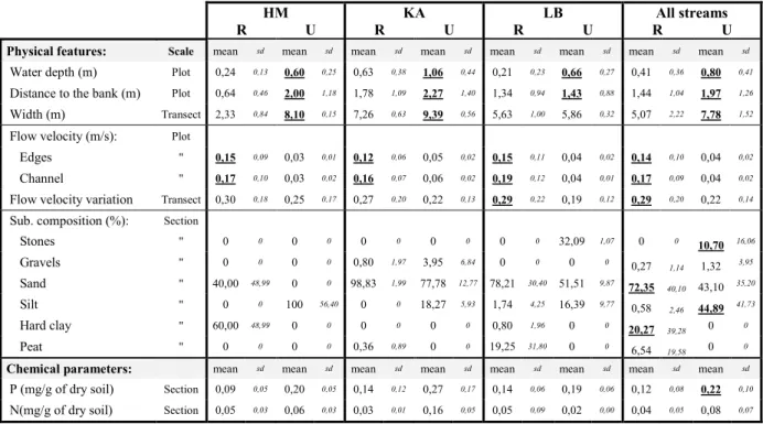
Physiochemical characteristics were compared between restored and unrestored reaches to assess the impact of restoration on stream habitats. The results are presented in table 5.
Table 5 : Physiochemical parameters of each stream; differences between restored and unrestored reaches were tested
within each streams (except for the substrate composition and the chemical parameters due to scant observations for these variables at this scale) and with all streams pooled (Wilcoxon test, P < 0,05);bold and underlined values indicate significantly higher values. “Sub” refers to substrate, “P” for available phosphorous and “N” for available nitrogen.
HM KA LB All streams
R U R U R U R U
Physical features: Scale mean sd mean sd mean sd mean sd mean sd mean sd mean sd mean sd
Water depth (m) Plot 0,24 0,13 0,60 0,25 0,63 0,38 1,06 0,44 0,21 0,23 0,66 0,27 0,41 0,36 0,80 0,41
Distance to the bank (m) Plot 0,64 0,46 2,00 1,18 1,78 1,09 2,27 1,40 1,34 0,94 1,43 0,88 1,44 1,04 1,97 1,26
Width (m) Transect 2,33 0,84 8,10 0,15 7,26 0,63 9,39 0,56 5,63 1,00 5,86 0,32 5,07 2,22 7,78 1,52
Flow velocity (m/s): Plot
Edges " 0,15 0,09 0,03 0,01 0,12 0,06 0,05 0,02 0,15 0,11 0,04 0,02 0,14 0,10 0,04 0,02
Channel " 0,17 0,10 0,03 0,02 0,16 0,07 0,06 0,02 0,19 0,12 0,04 0,01 0,17 0,09 0,04 0,02
Flow velocity variation Transect 0,30 0,18 0,25 0,17 0,27 0,20 0,22 0,13 0,29 0,22 0,19 0,12 0,29 0,20 0,22 0,14
Sub. composition (%): Section
Stones " 0 0 0 0 0 0 0 0 0 0 32,09 1,07 0 0 10,70 16,06 Gravels " 0 0 0 0 0,80 1,97 3,95 6,84 0 0 0 0 0,27 1,14 1,32 3,95 Sand " 40,00 48,99 0 0 98,83 1,99 77,78 12,77 78,21 30,40 51,51 9,87 72,35 40,10 43,10 35,20 Silt " 0 0 100 56,40 0 0 18,27 5,93 1,74 4,25 16,39 9,77 0,58 2,46 44,89 41,73 Hard clay " 60,00 48,99 0 0 0 0 0 0 0,80 1,96 0 0 20,27 39,28 0 0 Peat " 0 0 0 0 0,36 0,89 0 0 19,25 31,80 0 0 6,54 19,58 0 0
Chemical parameters: mean sd mean sd mean sd mean sd mean sd mean sd mean sd mean sd
P (mg/g of dry soil) Section 0,09 0,05 0,20 0,05 0,14 0,12 0,27 0,17 0,14 0,06 0,19 0,06 0,12 0,08 0,22 0,10
N(mg/g of dry soil) Section 0,05 0,03 0,06 0,03 0,03 0,01 0,16 0,05 0,05 0,09 0,02 0,00 0,04 0,05 0,08 0,07
Restored reaches are all shallower and have a significantly higher flow velocity (both in the channel and in the edges) than unrestored ones. They are also narrower, except in LB. Moreover, flow velocity variation is significantly higher in restored sections when all the streams are pooled. Restored reaches are mostly composed of sand (apart from HM that shows a higher percentage of hard clay), and feature only low percentages of stones, gravels, silt and peat. Substrate composition is more variable among unrestored sections, where gravels, hard clay and peat are either absent or not frequent. They always contain a higher silt percentage, especially in HM (100% of silt), which mainly causes the average percentage of silt to be higher than the percentage of sand in unrestored sections. Sand is still the main substrate in unrestored sections of KA and LB. Stones are only present in unrestored reaches of LB. Only available phosphorous concentration is higher in unrestored sections.
p. 11
B) Plants data 1) Species diversity
A total of 76 species were found in the three streams (appendix II-a). A PCA was first performed on the plant data (appendix III). As the individuals appear to be clearly spread according to their belonging to a stream, regional differences seem to have a strong influence on species composition so plant parameters differences were tested both within each stream and with all stream pooled.
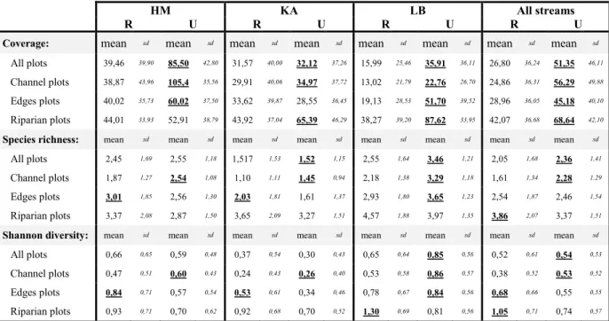
Table 6 : Plant parameters of each stream; differences between restored and unrestored reaches were tested within each
streams and with all streams pooled (Wilcoxon test, P < 0,05), bold and underlined values indicate significantly higher values.
HM KA LB All streams
R U R U R U R U
Coverage: mean sd mean sd mean sd mean sd mean sd mean sd mean sd mean sd
All plots 39,46 39,90 85,50 42,80 31,57 40,00 32,12 37,26 15,99 25,46 35,91 36,11 26,80 36,24 51,35 46,11
Channel plots 38,87 43,96 105,4 35,56 29,91 40,06 34,97 37,72 13,02 21,79 22,76 26,70 24,86 36,31 56,29 49,88
Edges plots 40,02 35,73 60,02 37,50 33,62 39,87 28,55 36,45 19,13 28,53 51,70 39,52 28,96 36,05 45,18 40,10
Riparian plots 44,01 33,93 52,91 38,79 43,92 37,04 65,39 46,29 38,27 39,20 87,62 33,95 42,07 36,68 68,64 42,10
Species richness: mean sd mean sd mean sd mean sd mean sd mean sd mean sd mean sd
All plots 2,45 1,69 2,55 1,18 1,517 1,53 1,52 1,15 2,55 1,64 3,46 1,21 2,05 1,68 2,36 1,41
Channel plots 1,87 1,27 2,54 1,08 1,10 1,11 1,45 0,94 2,18 1,38 3,29 1,18 1,61 1,34 2,28 1,29
Edges plots 3,01 1,85 2,56 1,30 2,03 1,81 1,61 1,37 2,93 1,80 3,65 1,23 2,54 1,87 2,46 1,54
Riparian plots 3,37 2,08 2,87 1,50 3,65 2,09 3,27 1,51 4,57 1,88 3,97 1,35 3,86 2,07 3,37 1,51
Shannon diversity: mean sd mean sd mean sd mean sd mean sd mean sd mean sd mean sd
All plots 0,66 0,65 0,59 0,48 0,37 0,54 0,30 0,43 0,65 0,64 0,85 0,56 0,52 0,61 0,54 0,53
Channel plots 0,47 0,51 0,60 0,43 0,24 0,43 0,26 0,40 0,53 0,58 0,86 0,57 0,38 0,52 0,53 0,52
Edges plots 0,84 0,71 0,57 0,54 0,53 0,61 0,34 0,46 0,78 0,67 0,84 0,56 0,68 0,66 0,55 0,55
Riparian plots 0,93 0,71 0,70 0,62 0,92 0,68 0,70 0,52 1,30 0,69 0,81 0,56 1,05 0,71 0,74 0,57
When all the streams are pooled, coverage is always higher in unrestored reaches,
regardless of the stream’s part considered. However, the difference is more pronounced in the
channel (where coverage is 2.3 times higher in the unrestored reaches) than in the edges (where coverage is only 1.6 times higher).
Unlike coverage, species richness and Shannon diversity show different pattern according the part of the stream considered. When all the streams are pooled, these parameters are also higher in unrestored stretches with all the plots pooled and in channel plots. The edge and riparian plots show an opposite result, with higher values in restored sections, although difference is not significant for species richness in edge plots. Within each stream, these differences were not always significant, and even reversed in LB’s edges plots.
p. 12
2) Growth forms diversity
As previously seen, coverage is significantly higher in unrestored reaches, so the following analyses were performed on growth form frequencies to reduce the induced bias. A PCA was also performed on growth forms data (appendix IV). As no clear tendency could be identified, growth forms frequencies between restored and unrestored reaches were also compared both within each stream and with all streams pooled (table 7). The differences were first graphically assessed (appendix V) with all plots pooled and then separating channel, edges and riparian plots. No clear different pattern arose within the different stream parts considered, so tests were performed only with all the plots pooled.
Table 7: Growth forms’ parameters; Wilcoxon test, P < 0.05, bold and underlined values represent the significantly
higher values.
HM KA LB All streams
R U R U R U R U
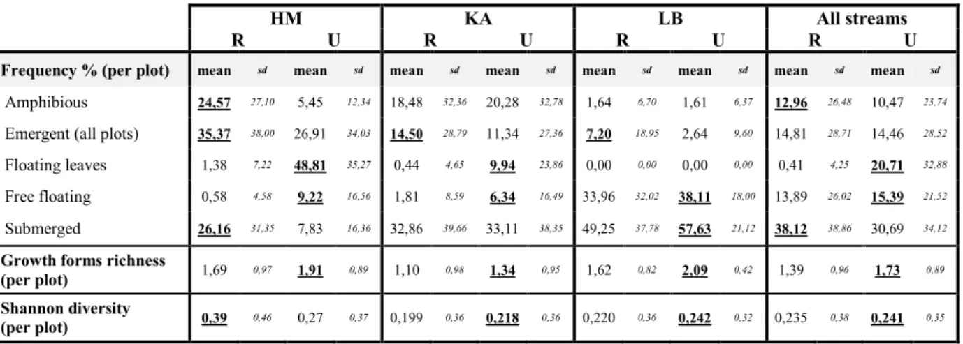
Frequency % (per plot) mean sd mean sd mean sd mean sd mean sd mean sd mean sd mean sd Amphibious 24,57 27,10 5,45 12,34 18,48 32,36 20,28 32,78 1,64 6,70 1,61 6,37 12,96 26,48 10,47 23,74
Emergent (all plots) 35,37 38,00 26,91 34,03 14,50 28,79 11,34 27,36 7,20 18,95 2,64 9,60 14,81 28,71 14,46 28,52
Floating leaves 1,38 7,22 48,81 35,27 0,44 4,65 9,94 23,86 0,00 0,00 0,00 0,00 0,41 4,25 20,71 32,88
Free floating 0,58 4,58 9,22 16,56 1,81 8,59 6,34 16,49 33,96 32,02 38,11 18,00 13,89 26,02 15,39 21,52
Submerged 26,16 31,35 7,83 16,36 32,86 39,66 33,11 38,35 49,25 37,78 57,63 21,12 38,12 38,86 30,69 34,12
Growth forms richness
(per plot) 1,69 0,97 1,91 0,89 1,10 0,98 1,34 0,95 1,62 0,82 2,09 0,42 1,39 0,96 1,73 0,89 Shannon diversity
(per plot) 0,39 0,46 0,27 0,37 0,199 0,36 0,218 0,36 0,220 0,36 0,242 0,32 0,235 0,38 0,241 0,35
Three clear differences between restored and unrestored reaches can be identified. Firstly, free floating species are always more frequent in unrestored sections. Secondly, floating leaves species are more abundant in unrestored reaches of HM, KA and with all streams pooled, while almost absent in the restored ones. In LB reaches, no floating leaves species were present at all. Thirdly, emergent species are always less abundant in unrestored stretches within each stream. However, when all streams are pooled together, there is no significant difference anymore.
For amphibious and submerged species, the results are less consistent between the streams. Amphibious species are more frequent in restored stretches of HM but there is no difference for KA and LB. Submerged species are also more frequent in restored reaches of HM, but there is no difference in KA and LB shows the opposite result (higher submerged species frequencies in unrestored reaches). Growth forms richness and diversity are always higher in unrestored stretches (except in HM for Shannon diversity).
p. 13
II) Relations between macrophyte communities and physical features
As the study focuses on the relations between macrophyte communities and physical features under restored circumstances, the following analyses were performed only on the restored plots (1979 plots).
A) Water depth and distance to the bank 1) Species diversity
First, the influence of substrate on plants parameters (i.e. coverage, species richness and Shannon diversity) was graphically assessed (appendix VI). Sand and hard clay showed a different influence on these parameters than stones, gravels, silt and peat (which altogether represent only 7.6% of the restored plots). Therefore, these plots were excluded and the analyses were performed on a subset of individuals including only plots with sand or hard clay, which are the main substrates in restored sections (1829 individuals).
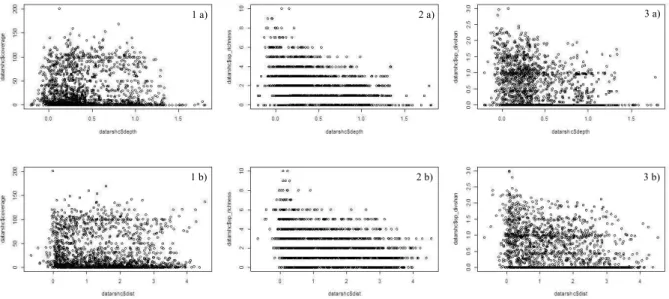
Plant parameters in relation to water depth and distance are presented in figure 2. The coverage doesn’t show any clear pattern whereas both species richness and Shannon diversity seem to decrease when both depth and distance to the bank increase.
Figure 2 : Relations between coverage (1), species richness (2) and Shannon diversity (3) and depth (a) and distance to the bank (b).
The results of the regressions are presented in table 8. No regression was found for the coverage. The relation between depth and distance to the bank and the regressions’ residuals are presented in figure 3.
1 a)
3 b) 2 b)
1 b)
p. 14
Table 8 : Results of the regressions on species richness and Shannon diversity.
Coverage: No regression
Species richness: Estimate Standard error Pr(>|z|) Explained
deviance: Intercept 1,20358 0,03169 <2e-16 *** 15,57% Depth -0,97157 0,12448 5,96e-15 *** Dist -0,13876 0,02781 6,05e-07 *** Depth : Dist 0,1064 0,05171 0,0396 *
Shannon index: Estimate Standard error Pr(>|t|) R²
Intercept 0,91287 0,03065 <2e-16***
0,1303
Depth -0,72609 0,09653 8,41e-14 ***
Dist -0,15048 0,02288 6,27e-11 ***
Depth : Dist 0,16855 0,03848 1,25e-05 ***
Figure 3 : (a) Relations between depth and distance to the bank / rho = 0.75, p-value < 2.2e-16; (b) Normal QQ-plot of GLM residuals (species richness); (c) Normal QQ-plot of lm residuals (Shannon diversity).
First, both depth and distance to the bank significantly influence species richness and Shannon diversity. The negative coefficients of both the variables indicate that species richness and Shannon diversity decrease when depth and distance to the bank increase. The coefficient of depth is higher (in absolute value) than the coefficient of distance, which implies that depth has a stronger effect on species richness and Shannon diversity than the distance to the bank. It can also be seen on figure 2 (2a and 3a) since the slopes are steeper on the graphs featuring the depth.
The positive interaction between depth and distance indicates that the influence of depth increases when the distance to the bank increases and vice-versa: far from the bank, the influence of depth is stronger than near it and in deep water, the influence of distance to the bank is stronger than in shallow water.
p. 15
However, depth and distance to the bank explain only 15,57% of species richness deviance and 13,03% of Shannon diversity variance. As no regression was found for the coverage, Spearman correlation coefficient was calculated for both depth and distance to the bank (table X).
Table 9 : Correlation coefficients between coverage and depth, and coverage and distance to the bank.
Coverage: Rho (Spearman) p-value
Depth -0,09823626 2,57E-05
Dist -0,1823293 3,90E-15
Both correlation coefficients are significant and negative, which indicates that when depth and distance to the bank increase, the coverage partly decreases. The correlation with the distance to the bank is higher than with the depth.
2) Growth forms diversity
As by definition, free floating species are not rooted in the stream bed, it is not relevant to study their relations with physical features such as water depth or distance to the bank. Thus, they were not included in this part.
- Coverage:
Figures 4 and 5 present the relations between the coverage of the different growth forms and depth and distance to the bank. Floating leaves species are not included because they are nearly absent from these reaches.
Figure 4 : Relations between the coverage of a) amphibious species, b) emergent species and c) submerged species with water depth.
p. 16
Figure 5 : Relations between the coverage of a) amphibious species, b) emergent species and c) submerged species with distance to the bank.
It is clearly visible that amphibious and submerged species develop in wider ranges of depths and distances to the bank than emergent species: the first ones are abundant until a 1,3 m depth, while emergent species don’t grow beyond a 1 m depth. Furthermore, amphibious and submerged species are present at all distances, whereas emergent species are abundant until ~1,8 m away from the bank (some rare individuals can be observed at 3,5 m). A correlation (Spearman correlation test) could be identified between emergent species’ coverage and depth and distance to the bank (table 10).
Table 10 : Correlation coefficients between emergent species’ coverage and depth and distance to the bank.
Coverage emergent: Rho (Spearman) p-value
Depth -0,4353176 < 2.2e-16
Distance to the bank -0.5812119 < 2.2e-16
The negative coefficients confirm what was graphically assessed: emergent species’ coverage partly decreases when depth and distance to the bank increase.
- Growth forms richness and Shannon diversity:
Figure 6 : Relations between 1) growth forms richness and 2) growth form diversity and a) depth and b) distance to the banks
a) b) c)
p. 17
In restored reaches, a maximum of four different growth forms were found per plot (figure 6). No regression was found for the richness or Shannon diversity although both graphs show a slight decrease of the parameters at higher depths and distances to the bank. Spearman correlation coefficients were thus calculated (table 11) and it appears that both growth forms richness and diversity are negatively correlated with depth and distance, with a higher coefficient (absolute value) for distance.
Table 11 : Correlation coefficients between growth forms richness and diversity and depth and distance to the bank.
Growth forms richness: Rho (Spearman) p-value
Depth -0,2688601 < 2.2e-16
Dist -0,3010803 < 2.2e-16
Growth forms diversity: Rho (Spearman) p-value
Depth -0,2166433 < 2.2e-16
Dist -0,2853236 < 2.2e-16
To investigate deeper the influence of depth and distance to the bank on growth forms richness, depth and distance of plots in which different numbers of growth forms were found were compared.
Figure 7 : Growth forms richness in relation to a) depth and b) distance; Kruskal-Wallis test followed by a multiple
comparison test (kruskalmc), P < 0,05.
Plots with three and four growth forms are on average significantly shallower and closer to the bank than plots than plots with fewer growth forms (figure 7). The average depths and distances of plots with three or for growth form are similar. Thus, in restored reaches, the highest number of growth forms is found in average in 21.5 cm deep water and 63.4 cm away from the banks.
a b c d d a a b c c
Number of growth forms Number of growth forms Depth (m)
p. 18
B) Influence of meanders
1) Comparison between bends and straight parts
Flow velocity variation, species richness and Shannon diversity were calculated at the transect level and then compared between bends and straight sections (figure 8).
Figure 8 : Comparison of a) flow velocity variation, b) species richness and c) Shannon diversity between bends (B) and straight parts (S); Wilcoxon test, P < 0,05.
Flow velocity variation is not higher in meanders than in straight parts. Moreover, species richness and Shannon diversity are not higher in bends either.
To test if flow velocity variation - regardless of bends or straights sections – has an
influence on plant parameters, the relations of flow variability with species richness and Shannon diversity were assessed. However, no regression or correlation was found (figure 9).
Figure 9 : Relationships between a) species richness and b) Shannon diversity and flow velocity variation
a a a a a a a) b) c) a) b) a a a a a a
p. 19
2) Comparison of inner bends, outer bends and straight edges
To assess the influence of meanders at a finer scale, edge plots of inner bends, outer bends and straight sections were compared (table 12).
Table 12 : Comparison of physical features, plant parameters and growth forms frequencies between inner bends, outer bends and straight edges; Kruskal-Wallis test followed by a multiple comparison test (kruskalmc), P < 0,05.
Inner bend Outer bend Straight edges
Physical features: mean sd mean sd mean sd
Depth (m) 0,16 a 0,21 0,27 b 0,25 0,21 c 0,21
Flow velocity (m.s-1) 0,12 a 0,08 0,13 a 0,08 0,16 a 0,11
Plant parameters: mean sd mean sd mean sd
Coverage (%) 18,30 a 29,52 35,77 b 41,20 31,51 b 35,23
Species richness 2,03 a 1,85 2,81 b 1,77 2,70 b 1,87
Shannon diversity 0,51 a 0,65 0,73 b 0,64 0,74 b 0,66
Growth forms frequencies (%): mean sd mean sd mean sd
Amphibious 7,03 a 17,42 9,20 a 18,35 8,95 a 18,01
Emergent 26,97 a 36,72 24,65 a 32,05 31,05 a 35,15
Submerged 23,47 a 32,43 40,43 b 36,23 33,38 c 36,07
Growth forms richness 1,38 a 1,06 1,85 b 0,97 1,67 b 1,00
Growth forms diversity 0,27 a 0,41 0,37 b 0,46 0,34 b 0,42
Depth is significantly different in each edge category: outer bends are the deepest and inner bends the shallowest. Flow velocity doesn’t vary between the categories. Coverage, species richness and Shannon diversity are always lower in the inner bend plots, and are similar in outer bends and straight parts. Growth forms richness and diversity show the same pattern. Amphibious and emergent species frequencies are similar in each category. Submerged species are the most frequent in outer bends and the least frequent in inner bends. Floating leaves species were nearly absent from restored reaches and therefore not included in this analysis.
p. 20
DISCUSSION
I) A contrasted response of species diversity between stream channel and edges
On the one hand, when all the plots (i.e. channel, edge and riparian plots) are pooled, coverage, species richness and Shannon diversity are always higher in unrestored reaches. Coverage is also always higher in
unrestored streams in the different
categories of plots. As the restoration measures were carried out in 2010 and 2011, macrophytes might not have had time enough to fully develop in restored reaches. Indeed, after restoration, substrate
is left completely bare (figure 10), so, in 2013, plant communities might still be in an early colonisation stage featuring small individuals. On the other hand, unrestored reaches were channelised decades ago and thus feature fully established macrophytes communities with bigger and more competitive individuals. Moreover, available phosphorous being higher in unrestored reaches, the difference in nutrients availability could also play a role in this coverage difference. Other studies show various results in terms of coverage recovery after restoration: Baattrup-Pedersen et al. (2000) observed a re-colonisation of 10% two years after restoration, while Henry et al. (1996) found a total re-colonisation after the same time span. These results support the hypothesis that studied restored reaches might still be in the process of re-colonisation and show that it is difficult to conclude about the average time span after which plants coverage would reach a pre-disturbance level. This span is likely to be influenced by propagule source proximity (Pedersen et al., 2006).
Furthermore, species richness and Shannon diversity show a different pattern when the different plot categories are separately analysed. In edge and riparian plots, they are higher in restored reaches. It can be explained by more suitable habitats induced by restoration, since restored stretches are shallower and narrower (table 5) and that plant diversity decreases with both depth and distance to the bank (table 8).
However, the bare substrate resulting of restoration left plenty of room for pioneer species to colonise the reaches, whereas the later successional stage of unrestored stretches features fewer but more competitive species. For example, some unrestored banks feature large and
p. 21
dense stands of Carex sp. and Glyceria maxima among which nothing else can grow. Moreover, Verdonschot & Nijboer (2002) show that the number of species can increase in the first years after restoration, but then start to decrease due to a high input of nutrients as a consequence of rich sediments depositing on the banks. Thence, these results have to be considered with caution.
In channel plots, on the opposite, species richness and Shannon diversity are higher in unrestored stretches (the higher number of channel plots explains why plant parameters are always lower in restored reaches when they are all pooled) . Moreover, in restored reaches, channel plots’ coverage represents 44% of the unrestored coverage, whereas it represents 64%
of the unrestored coverage in the edge plots. Thus, the improvement of physical habitat didn’t
benefit yet to the restored channels. These results imply that colonisation is faster on the edges of the streams than in the channel, as also shown by (Henry et al., 1996). It can be explained by the hydromorphological differences between the channel, usually deeper, and the edges, usually shallower and by definition closer to the banks.
Indeed, free flowing diaspores due to instream dispersal are more likely to be deposited next to the banks, where the flow velocity and depth are lower than in the channel and where the stream bed is more likely to become dry because of water table fluctuation. Furthermore, lateral dispersion from the bank (mainly through plant ingrowth) contributes to a higher species richness in stream edges (Pedersen et al., 2006). Depth also affects aquatic plant communities: light availability playing an important role in seed germination (Fenner & Thompson, 2005), diaspores are more likely to germinate and expand in shallow water where light is less attenuated. However, the influence of distance to the bank is altered by the water depth and reciprocally, as shown by their significant interaction (table 8). A possible explanation is that, in deep water, clonal growth from bank plants might allow them to settle in depths where they are usually absent or really rare, but not towards the channel. On the other hand, shallow water might enable them to expand further from the bank (figure 11).
p. 22
Finally, a channel usually features faster flow velocities than on the stream edges, which can induce plant uprooting or breakage, and thereby hamper macrophyte development (Franklin et al., 2008).
II) Differences in response according to growth forms
The distinct growth forms responded differently to restoration. When all the streams were pooled, amphibious and submerged species were more frequent in restored sections. Within each stream, emergent species were also more abundant in restored reaches. On the contrary, free floating and floating leaves species were more frequent in unrestored stretches. These different responses are mainly due to the habitats requirements of the growth forms.
The higher frequencies of amphibious species in restored reaches appear to be mainly due to the influence of HM (table 7). Their lower frequency in unrestored reaches of HM might be due to the fact that they are outcompeted by emergent species next to the banks, and by floating leaves species in the channel, which would leave them with little room left to develop. In the two others streams, they are equally abundant in restored and unrestored reaches, probably because they suffer less from competition (fewer or no floating leaves species) and also because they can develop in a wide range of depths.
Submerged species such as Callitriche sp. and Elodea nuttalli are usually good colonisers since they show a large capacity to disperse by free-floating shoot fragments (Baattrup-Pedersen et al., 2003). Consequently, they could easily establish in the bare substrate of restored reaches, while they might have been outcompeted by floating leaves in unrestored stretches. Thus, it could explain their lower frequencies in unrestored reaches of HM, and their higher frequencies in unrestored stretches of LB, where floating leaves species are completely absent. In KA, floating leaves species seem not to be abundant enough to influence submerged species.
The higher emergent species frequencies in restored sections can be explained by a more suitable habitat in restored stretches: indeed, they mostly occur in shallow water and close to the banks (figures 4 and 5) and restored reaches are shallower and wider. Additionally, ingrowth from the banks (which might me more pronounced in shallower and narrower restored sections) is likely to increase emergent frequency since banks feature mostly terrestrial plants.
p. 23
Floating leaves species such as Nuphar lutea and Potamogeton natans are usually competitive species (Bornette & Puijalon, 2011) and thus occur in late stages of plant succession, with a low disturbance level. As they thrive in non-frequently disturbed environments, the higher flow velocity in restored reaches might hamper their development. As shown in table 7, floating leaves species frequencies show noteworthy differences between the unrestored reaches of the three streams: they show an average of 50% in HM, whereas it drops to respectively 10% and 0% in KA in LB. These differences might be due to different regional species pools or / and variable management intensities within each stream. Indeed, unrestored reaches of HM are a 100% composed of silt (which typically occurs in late successional stages because of the trapping of particulate matter by plants, Bornette & Puijalon, 2011). On the opposite, KA and LB substrate are only composed of 18% and 16% of silt. Thus, it can be assumed that LB and KA are more intensively managed (by cutting or dredging) than HM.
Finally, the faster flows in restored sections can cause free floating to be flushed away, whereas very low flow velocity in unrestored reaches is likely to favour them, hence their higher frequency in the last ones.
Thus, restoration shows beneficial, negative or non-clear impact on the different growth
forms, depending on their optimal habitats.
Higher growth forms richness and diversity were found in unrestored reaches mainly because floating leaves species were nearly absent of restored section. These parameters were negatively correlated with both depth and distance to the bank and plots with higher growth forms richness (i.e. with 3 and 4 different growth forms) were in average located in 21.5 cm deep water and 63.4 cm away from the banks. It is due to the fact that, as shown in figures 4 and 5, all growth forms can potentially grow in these conditions whereas emergent plants don’t occur in deep water and places far from the banks.
III) A relative influence of meanders
The aim of the creation of meanders is to enhance habitat heterogeneity by increasing and more equally distributing the surface area per range of depth (figure 12) and by inducing a higher flow velocity variation. The resulting more varied niches are then expected to increase plant diversity (Palmer 2005). However, as shown in figure 8, flow velocity variation, species richness and Shannon diversity are not higher in meanders than in straight sections.
p. 24
This absence of difference could be due to the fact that straight restored stretches feature lower bank slopes than unrestored ones and thus more evenly distributed surface areas per range of depth (pers. obs.), as illustrated in figure 12. Thus, it would have been relevant to calculate depth variation among transects to verify this hypothesis.
Figure 12 : surface area per range of depth according to different stream bed profiles.
Another explanation would be that more suitable habitats (i.e. shallower and closer to the banks) have a higher impact on diversity than heterogeneity, which could also explain why flow velocity variation could not be related to species richness or Shannon diversity. Indeed, Biggs et al. (2001, in Pedersen et al., 2006) found that the higher macrophyte richness in restored sections was not linked to the enhanced habitat heterogeneity but to shallow water. Similar results were also found for macroinvertebrates communities (Palmer et al., 2010), which questions the previously assumed role of heterogeneity in instream biota.
But, morphological adjustments in recently reshaped streams can induce a high sediment
mobilisation and deposition and thus obscure plant communities’ response to restoration.
Moreover, field observations showed that morphological characteristics of meanders (shallower inner bend and deeper outer bend) didn’t always occur in the actual meander but were more significant further downstream and even sometimes in straight parts consecutive to meanders. Thus, the study design (that focused on the centres of meanders) could have biased the results. Finally, species richness and Shannon diversity were only calculated at a transect level. It could have been interesting to calculate them at a section level to check if there is still no difference between meanders and straight parts.
Even though meanders don’t show an overall higher diversity, they influence plant communities on a fine scale.
Coverage, species richness and Shannon diversity appear to be significantly lower in inner bend, (and no different between outer bends and straight edges), which is in contradiction with the results of the regressions that show that species richness and Shannon