Capacity Factor Risk At Nuclear Power Plants

by

November 2010 Yangbo Du and John E. Parsons

Capacity Factor Risk At Nuclear Power Plants

CAPACITY FACTOR RISK AT NUCLEAR POWER PLANTS

Yangbo Du

and John E. Parsons

November 2010

We develop a model of the dynamic structure of capacity factor risk. It

incorporates the risk that the capacity factor may vary widely from year-to-year, and also

the risk that the reactor may be permanently shutdown prior to the end of its anticipated

useful life. We then fit the parameters of the model to the IAEA’s PRIS dataset of

historical capacity factors on reactors across the globe. The estimated capacity factor

risk is greatest in the first year of operation. It then quickly declines over the next couple

of years, after which it is approximately constant. Whether risk is constant or increasing

in later years depends significantly on the probability of a premature permanent

shutdown of the reactor. Because these should be very rare events, the probability is

difficult to estimate reliably from the small historical sample of observations. Our base

case is parameterized with a conservatively low probability of a premature permanent

shutdown which yields the approximately constant variance. Our model, combined with

the global historical dataset, also yields relatively low estimates for the expected level of

the capacity factor through the life of the plant. Our base case estimate is approximately

74%. Focusing on alternative subsets of the data raises the estimated mean capacity

factor marginally, but not significantly, unless the sample chosen is restricted to selected

countries over select years. This emphasizes the need for judgment in exploiting the

historical data to project future probabilities.

* _{Center for Energy and Environmental Policy Research, MIT, E19-411, 77 Massachusetts Ave.,}

Cambridge, MA 02139 USA, E-mail: yangbodu@mit.edu

** _{Corresponding author: MIT Sloan School of Management, MIT Center for Energy and Environmental}

Policy Research, and the MIT Joint Program on the Science and Policy of Global Change, MIT, E19-411, 77 Massachusetts Ave., Cambridge, MA 02139 USA, E-mail: jparsons@mit.edu

1. INTRODUCTION

One of the critical risks facing an investor in a nuclear power plant is uncertainty

about the plant’s realized capacity factor. Realized capacity factors show great variation.

Although the typical investor’s cash flow model of a proposed plant shows a projected

capacity factor of 85% or more, many reactors have problems achieving this target.

Oftentimes the shortfall is quite large. According to the Power Reactor Information

System (PRIS) database maintained by the International Atomic Energy Agency (IAEA),

the realized capacity factor is less than 50% in more than 10% of all reactor years in their

database. In one of the countries with the largest nuclear power programs, Japan, the

three most recently constructed plants have been marked by major operational problems

that have kept their lifetime capacity factors at 63%, 77% and 34%. Several other units in

Japan were recently shutdown for over two years due to an earthquake. The average

capacity factor in Japan for 2007-2009, the most recent period for which data are

available, lies at 61%. In the US, performance was extremely poor in the 1970s and

1980s. For example, in 1985 the overall capacity factor for nuclear power plants in the

US was 58%. Individual reactor performance varied widely. Subsequently, capacity

factors in the US have climbed markedly, so that the average is now slightly above 90%.

How should capacity factor risk impact the valuation of a prospective new build

power plant? Few economic analyses address this question explicitly. The standard

discounted cash flow model simply applies a single risk-adjusted discount rate to the

aggregate cash flow line, discounting successive year’s cash flows by the compounded

discount rate. Although not widely appreciated, this simple model embodies a very

restrictive implicit assumption about the dynamic structure of risk at the level of the

aggregate cash flow: that is, the risk or variance of the cash flow grows linearly with

time. This structure is consistent with the risk being well described as a geometric

Brownian motion, but is not consistent with many other dynamic risk structures. Capacity

factor risk is unlikely to be well described by a geometric Brownian motion. Uncertainty

on the capacity factor parameter will almost certainly not grow linearly with time. But

what is the dynamic structure of capacity factor risk? Answering this question is a

prerequisite to turning to more advanced valuation techniques, such as a real options

model or similar tools.

In this paper we provide a fully specified model of the dynamic structure of

capacity factor risk. We then fit the parameters of the model to the IAEA’s PRIS dataset

of historical capacity factors on reactors across the globe.

We find that capacity factor risk is greatest in the first year of operation, declining

quickly in the next couple of years. In later years, regardless of parameterization, capacity

factor risk never again rises to the level attained in the early years. Whether risk is

constant or slightly increasing in later years depends significantly on the probability of a

premature permanent shutdown of the reactor.

In fitting our model, we also obtain estimates on the expected level of the capacity

factor through the life of the plant. Our estimates are very low relative to the 85% or

higher figures commonly employed in investor cash flow models. We examine various

subsets of the data to account for possible factors that could bias our numbers to a low

1 _{An example of the application of these more sophisticated techniques appears in Rothwell (2006),}

which is an application of the real options technique to the valuation of a new nuclear build. However, Rothwell continues to rely upon the Brownian motion assumption although certain key risk factors—such as the capacity factor and the electricity price—clearly do not fit this assumption. Another example of these more sophisticated techniques appears in Samis (2009). He focuses on the structure of electricity price risk,

level. These do argue for a slight upward adjustment in the expected level of the capacity

factor through the life of the plant, but the adjustments are small and the final estimate

remains well short of the 85% mark, unless the sample chosen is restricted to selected

countries over select years.

There is a large literature analyzing the determinants of the capacity factor.

Joskow and Rozanski (1979) estimate a significant learning curve for the operator, with

the expected capacity factor increasing significantly in the first years of operation. They

also document some learning by the manufacturer as successive plants of the same design

are produced. They document some difference in the learning curve by reactor design,

but essentially no difference across countries. Finally, they noted that the larger reactor

designs had lower capacity factors. Easterling (1982) estimates that the learning effect on

capacity factors is greatest during the first five years of operation. The variability of

capacity factors is highest in the first year. He notes that different designs have different

mean capacity factors, and that there are persistent differences in the individual unit

capacity factors that could possibly represent any number of other factors. Krautmann

and Solow (1988) find that the age of the unit, its vintage, the size of the unit, and the

past year’s capacity factor are all significant determinants of the expected capacity factor.

Rothwell (1990) refines the observation of the capacity factor by organizing the data

according to the frequency for refueling, which need not be annual, the frequency used in

most analyses. He also decomposes the capacity factor into the service factor—i.e.,

whether the unit is available or has been taken down for refueling or for repair—and the

capacity utilization when operating. Finally, he segments the dataset by manufacturer.

The results for age are very mixed across manufacturers, and so he argues it should not

be used to estimate the expected capacity factor. Similarly, the results for size seem to

relate to specific designs and not to size generally.

Krautmann and Solow (1992) show

that improvements in the expected capacity factor with the age of the unit appear to have

exhausted themselves in the period following the Three Mile Island accident, and that the

units of at least one design were on the declining side of the age-performance curve.

Lester and McCabe (1993) find a learning curve effect in the first three years of a units

operation, and then document the differential learning curves for units operated at the

same site, as well as the role of experience by design, by company and for the industry as

a whole. Sturm (1993) identifies declining performance with age for countries in the

former Soviet Union and Eastern Europe, especially attributable to the years immediately

following the political transformations of the late 1980s and early 1990s. This is in

contrast to the improving performance with age in the West at the same time, and even

with identical reactor designs. Noting the significant improvements in the capacity factors

among US nuclear power plants, Rothwell (2000) provides an updated estimate of the

expected capacity factors by design type, manufacturer and size of the unit. Rothwell

(2006) updates this for one cohort. Koomey and Hultman (2007) also note the significant

improvement in the mean capacity factor at US units.

Our contribution to this literature is our focus on the variability in the capacity

factor and the risk structure through time.

2 _{There is related work on factors that one might expect to enter as a determinant of the capacity factor.}

For example, Roberts and Burwell (1981) estimate the learning curve in licensee events reports and how this is impacted by placing new reactors at the same site as existing reactors. A lower number of events may lead to an increased capacity factor, although the authors did not report on capacity factors. David Maude-Griffin and Rothwell (1996) document how the hazard rate for an unplanned outage declined after the Three-Mile-Island reactor incident and the ensuing regulatory policy changes. Sturm (1994) also evaluates the time between forced outages, and finds significant country differences. Within country no

A portion of the previous literature touches on the variability in the capacity

factor, including the random process of unplanned shutdowns and the decision to

permanently shutdown a reactor. Rothwell (2007) incorporates a measure of the volatility

in the capacity factor into his valuation model. It appears that volatility is estimated as if

the factor were generated by a Brownian motion. Sturm (1995) estimates nuclear power

production at a plant as a controlled stochastic process. The technology defines certain

tradeoffs facing plant managers, and these managers make choices in operating the plant

to optimize an objective function. This yields an estimated stochastic process for

unplanned outages and plant capacity when operating. Given the complexity of the

problem, the data used for estimating the model is chosen from a narrow time window

likely to reflect a stable technology and objective function. Rothwell and Rust (1995)

estimate a similar type of model in order to estimate the endogenous decision to

permanently shutdown a plant. Rothwell (2000) also estimates the differential likelihood

of different US plants being permanently shutdown as the regulatory environment shifts.

Our paper does not report the volatility or likelihood of a shutdown estimated

from an optimization problem. We model the capacity factor risk structure as if the

capacity factor were an exogenous variable.

2. THE DATA

The IAEA’s PRIS database reports a variety of data on individual reactors

throughout the world, including annual performance data.

Table 1 shows some summary

3 _{Although the data is available on-line, the mode of access currently makes it inconvenient to acquire a}

complete overview of the data. Upon request, the IAEA provided us the data in a convenient spreadsheet form, and we have posted that on our website together with this paper so that others can easily access the same data. See: web.mit.edu/ceepr/www/publications/workingpapers.html

information on the PRIS data. As of year-end 2008, the database included information on

535 reactors that had operated for some subset of years since 1969. Of these, 428 were in

OECD countries, while 107 were in non-OECD countries. For calendar year 1969 the

database includes information on only a single operating reactor. This number grows

quickly to a maximum of 444 operating reactors included in the database in 2005.

Obviously, early in the database the reactors included are young: the median age of

operating reactors is less or equal to 5 years through 1978, growing to 10 years in 1990,

and reaching 25 years in 2008.

PRIS reports a variety of data on a reactor’s operating performance, including the

portion of time the reactor was on-line, the total energy generated, the energy lost due to

planned outages, the energy lost due to unplanned outages and the energy lost due to

external factors. PRIS also reports a reference level of energy generation, which is a

measure of the nameplate capacity of the unit. These variables can be combined to

calculate a number of different versions of a capacity factor. Discrepancies between the

different versions tend to occur because they each reflect differently events in which the

plant’s potential generating capacity differs from its reference power rating due to factors

outside the control of the plant operator. These factors include but are not limited to

ambient temperature, which affects the plant’s thermal efficiency, and periods of low

electricity demand that do not result in complete utilization of a plant’s electricity output.

Higher generating potential arises during periods of colder temperatures relative to that of

the plant’s nameplate capacity, which increases the plant’s heat sink capacity and in turn

4 _{Although the PRIS database of capacity factors is relatively comprehensive, it turns out that the}

capacity factors for a few reactors are missing. We did not investigate or try to resolve these few missing observations.

its power output. Therefore output may be greater than capacity. Examples of this are

widespread among units reporting high capacity factors, notably in South Korea where at

least one reactor operated at above 100 percent nameplate capacity for every year since

1993 except for 1995 and 2007. One version of a capacity factor will reflect this,

recording a capacity factor above 100%, while another version will adjust the baseline

capacity to reflect the higher potential and record a capacity factor of 100%. Conversely,

in a country like France where nuclear capacity exceeds base-load demand, inevitably

some units are forced to follow load and cut generate below capacity although the plant is

fully available. One version of a capacity factor will reflect this lower generation, while

another version will adjust the baseline capacity to reflect the external constraint. In

France in 2008, where nuclear power supplies over three-quarters of electricity output,

the average capacity factor as measured by one version, the Load Factor, was a full two

percentage points below the average capacity factor as measured by another version, the

Energy Availability Factor — 75.9 percent versus 77.9 percent respectively.

To formalize this discussion, we provide the definitions of various elements in the

calculation of capacity factors, and the formulas for different versions of capacity factors.

These are the definitions as provided by the IAEA’s PRIS dataset:

 T – Reference period – time from beginning of period, first electrical

production (for units in power ascension), or start of commercial operation

(for units in commercial operation), whichever comes last, to the end of

the period or final shutdown, whichever comes first

 t – On-line hours – hours of operation (breakers closed to the station bus)

during the reference period

 OF – Operating factor (%) = t/T×100

 RUP – Reference unit power (MW) – Maximum electrical power output

maintained during prolonged operation at reference ambient conditions,

 REG – Reference energy generation (MWh) = RUP×T

 EG – Energy generated – net electric energy output after subtracting

station load (electric energy drawn by the power station’s components)

 LF – Load factor (%) = EG/REG×100

 PEL – Planned energy loss – energy not produced during the reference

period due to planned outages (foreseen at least four months in advance)

during refueling and other operations and maintenance activities

 PUF – Planned Unavailability Factor = PEL/REG

 UEL – Unplanned energy loss – energy not produced during the reference

period due to unplanned outages (foreseen less than four months in

advance) internal to the plant

 UUF – Unplanned Unavailability Factor = UEL/REG

 UCF – Unit capability factor (%) = (REG – PEL – UEL)/REG×100

 XEL – External energy loss – any energy loss due to causes external to the

plant

 XUF – External Unavailability Factor = XEL/REG

 EAF – Energy availability factor (%) = (REG – PEL – UEL –

XEL)/REG×100

To illustrate how the different versions of capacity factors reflect the specific

situation of different units, Table 2 shows the data for four different reactors as reported

in 2007. Column E shows the Genkai 4 Unit in Japan. It operated 100% of the time, so

that its Operating Factor was 100%. However, its Load Factor was 101.5%. This is

because the Energy Generated was more than its Reference Energy Generation, i.e. the

ambient conditions in that year produced an actual capacity greater than the nameplate or

reference capacity. Its Energy Availability Factor was 100%. This demonstrates the

difference between the LF and the EAF. The LF reflects actual energy produced as

against a reference or nameplate capacity, although the actual capacity may be higher or

lower than the reference. In contrast, the EAF is normalized by whatever is the actual

capacity of production. Therefore the EAF cannot be greater than 100%. Column F

shows the Sequoyah 1 Unit in the United States. This unit operated 87.5% of the time,

with 12.5% of the time down for planned outages. When it was operating, it must have

been operating at full capacity since the EAF equals the OF. The LF is lower than the

EAF, which must be because actual capacity across the hours of planned operation was

less than the reference capacity. Column D shows the Wolsong 4 Unit in Korea. This unit

operated 93.1% of the time. However, the EAF is only at 92.8%, so during some portion

of the time it was operating it must have done so at slightly less than full capacity. Most

of the time it was not operating was for planned outages, although a small portion was for

unplanned outages. Column C shows the Cattenom 1 Unit in France. In addition to the

planned and unplanned outages, there is a portion of its generation capacity that is

unutilized, 1.5%, because of external factors. This is likely due to the need in France to

operate some units in a load following mode, i.e. to not take the full capacity of the unit

even when it is made available to the system. Therefore, the UCF is higher than the EAF.

In our analysis below we focus exclusively on the variable called “Load Factor”

(LF), so for the remainder of this paper the reader should treat the term Load Factor as

synonymous with capacity factor. Table 3 shows how the median Load Factor has

evolved over time, growing from the 60% range in the early 1970s to approximately 85%

in the 2000s. The standard deviation of the annual Load Factors has not changed very

much over time, fluctuating modestly around 22% throughout the life of the database.

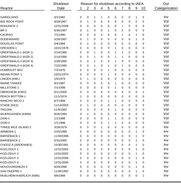
Importantly, the database includes the time series of performance data on reactors

that have since been permanently shutdown. There are 98 reactors in the database that

had been permanently shutdown as of 2008. Table 1 shows the annual number of

shutdown reactors, together with the cumulative number of shutdown reactors through

time. The large majority of these shutdowns occurred because the reactor has reached the

end of its useful life, or has become technologically outdated, or because economic

factors no longer make it worth operating. A few of these shutdowns occur because of

accidents or other operational problems. The database provides some information on

these reasons, although it is useful to have more detail on each case.

We will return later

to examine more carefully the issue of reactors that are both temporarily and permanently

shutdown.

3. A STOCHASTIC MODEL OF THE CAPACITY FACTOR

Denote a nuclear power plant’s capacity factor in year t as F

. Denote by T the

number of years in the normal economic life of the plant—for example, the normal

economic life may be 40 or 60 years. Then the profile of the capacity factor over the life

of the plant, t=1,…T, is, F

,…,F

. We assume that in each year, the capacity factor can

take on only the integer values from 0% to 100%. In addition, we assume that the plant

may permanently shut-down, despite not having yet reached the end of its normal

economic life, i.e., despite the fact that t≤T. We call this a premature permanent

shutdown. Once a plant is permanently shutdown, it cannot be restarted, so there is a

difference between a capacity factor of 0% and the state of being permanently shutdown.

We model the evolution of the capacity factor over the life of the plant as a

stochastic process. This allows us to reflect correlation between the capacity factors

5 _{The IAEA provides separate information on permanently shutdown reactors. This shows a total of 123}

permanently shutdown reactors. Of these, 7 were shutdown prior to 1969, and so would not be included in our dataset. That leaves 116 reactors that were permanently shutdown and that would appear in our dataset. Of these, 2 were shutdown in 2009, and so we do not treat them as shutdown as of 2008 when our data ends. That leaves 114 reactors that were permanently shutdown as of 2008 and that would appear in our dataset. We can only identify 99 of these, leaving 15 unaccounted for. These are reactors for which no capacity factor data appeared in the PRIS database. Omitted these will underestimate the probability of shutdown.

across years. For example, a plant currently operating at 50% capacity factor may be

more likely to operate at 50% in the next year than is a plant currently operating at 95%.

We initially assume that the probability distribution for the capacity factor at t is

conditioned only on the capacity factor at t-1, and so is independent of the age of the

plant. Obviously, one could make a case that the distribution might vary according to the

reactor’s age, and we will revisit this possibility later in the paper.

Let i be the capacity factor in year t-1 and j be the capacity factor in year t,

i,j

{0%,1%,…,100%}{“shutdown”}. Define



as the probability that the capacity

factor in year t equals j, given that the capacity factor in year t-1 equals i. That is,



is

the probability of transitioning from i to j. Denote by



the 102102 transition matrix

with elements



, i,j{0%,1%,…,100%}{“shutdown”}. We assume the probability



is a mixture of two distributions: the probability of a permanent shutdown, and, given no

permanent shutdown, the probability of transitioning from one integer capacity factor

value to another. Define



as the probability that the plant is permanently shutdown in

year t, given that the capacity factor in year t-1 equals i. Define



as the probability that

the capacity factor in year t equals j, given that the plant is not permanently shutdown in

year t, and that the capacity factor in year t-1 equals i. Then the probability that the

capacity factor in year t equals j, given that the capacity factor in year t-1 equals i, is



























shutdown

=

j

,

,

i

for

θ

,

j

i,

for

θ

φ

=

π

99%,100

0%,1%,...

99%,100

0%,1%,...

1

.

For t=1, the first year of operation following the start-up, there is no prior year capacity

factor, and so we must define the first year’s probability distribution separately. We

denote this distribution as



. It is similarly composed as a mixture of two

distributions, and we label these elements as



and



. We denote by



the full

102101 conditional transition matrix with elements



,

i

{“start”}{0%,1%,…,100%}, j{0%,1%,…,100%}. We denote by



the 1021

matrix of shutdown probabilities,



, i{“start”}{0%,1%,…,100%}.

In order to capture the volatility of the capacity factor transitions, and to impose

some regularity on the structure of the elements of the conditional transition probability

matrix,



, we assume that



is a Beta-binomial distribution with n=100 and parameters



(F

) and



(F

). When we estimate



and



, we will make some regularity assumptions

on how the parameters may vary with the capacity factor, i{0%,1%,…,100%}.

This simple structure enables us to calculate a time profile of stochastic capacity

factors for a new build nuclear power plant. Define p

as the unconditional probability

that the capacity factor in year t equals j. Denote by P the T102 matrix with elements

p

, t=1,…T, j{0%,1%,…,100%}{“shutdown”}. The first row of P is the first year’s

probability distribution, p

=



. We can derive the successive rows by successive

matrix multiplication using



:

Π

p

=

p

,

where p

is the t

row of P, with 1102 elements, p

is the previous row of P, with

4. ESTIMATION FROM THE RAW DATA

We organize the sample data into a transition matrix by populating the elements

of the matrix with a simple count of the observed transitions. Reactor-by-reactor, we

simply count the number of year-to-year transitions from capacity factor i to capacity

factor j, and sum across all reactors. In the PRIS database, capacity factors are reported to

the 12th decimal place. In doing our count, we round down to the nearest integer.

Therefore, the row denoted by 90 percent includes all capacity factors from 90 percent up

to, but strictly less than 91 percent. An exception to this rule applies for reactors

operating above 100 percent capacity factor, which are classed in the 100 percent level

regardless of the margin the actual power generation exceeds the reference power

generation. Count values in each row are then normalized to a sum of one by dividing

each row entry by the sum of the count values for the row. We call this the sample

conditional probability matrix,



. Table 4 shows an extract of this sample

conditional transition matrix constructed using the complete capacity factor data available

from PRIS through 2008. Figure 1 is a graphical display of the matrix.

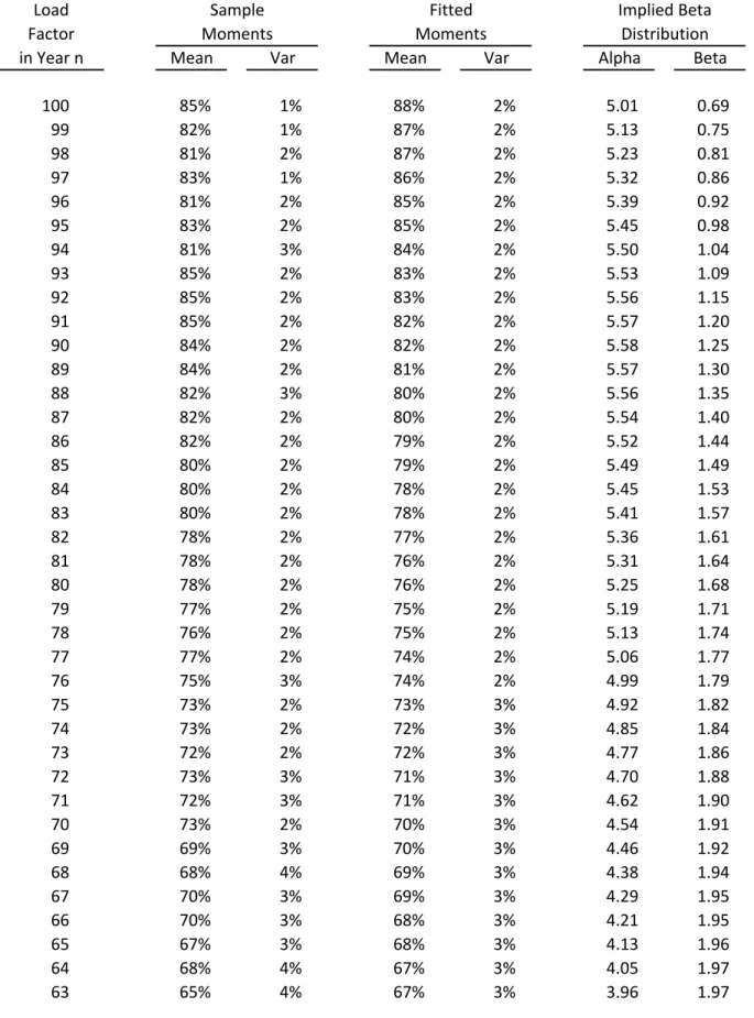
We use this sample to estimate the underlying probability distribution. Table 5

shows the conditional sample mean capacity factor in year t, given each capacity factor in

year t-1,



=

j

φ

φ

, i{0%,1%,…,100%}. These values are also plotted in

Figure 2. Clearly the conditional expected capacity factor in year t is increasing as a

function of the capacity factor in year t-1. Table 5 also shows the sample variance of the

capacity factor in year t, given each capacity factor in year t-1,









0 2 = j sample j i, sample i

φ

φ

j

,

is a declining function of the capacity factor in year t-1. This indicates a tendency for

reactors already performing at a high capacity factor to maintain such performance with

relatively low variability. Reactors performing at lower capacity factors at any given

year tended to exhibit more variable performance the following year. This characteristic

is also apparent in Figures 2 and 3.

From these sample conditional means and variances we estimated the underlying

distribution means and variances by regressing the log of the sample mean and the log of

the sample variance onto the initial capacity factor. Table 6 reports the results of this OLS

regression with robust standard errors. Table 5 shows the fitted moments at each capacity

factor using the parameter estimates from the regression in Table 6. From these fitted

moments we generate the distribution parameters alpha and beta using the

method-of-moments.

Table 5 reports the resulting alpha and beta parameters at each initial capacity

factor. Figure 4 illustrates the results by displaying three probability distributions

associated with three different initial capacity factors. Each distribution describes the

probability of the capacity factor in year t given its respective capacity factor in year t-1,

as marked. The pattern described above—in which reactors already performing at a high

capacity factor tend to maintain such performance, while reactors performing at lower

capacity factors at any given year tend to exhibit more-variable performance the

following year—is reflected in the resulting conditional implied Beta distributions.

In order to recover the conditional probability distribution at the start-up, we

follow a similar procedure. However, since we only have one distribution to calculate,

6 _{The implied parameters of the distribution,  and , are solved for using the fitted mean, , and the}

there is no need to impose any regularity across different starting capacity factors, and so

we skip the OLS step. Instead, we directly apply the method of moments to the sample

conditional mean,



=

j

φ

φ

, and sample conditional variance,









φ

φ

j

. The results are included at the bottom of Table 5.

We estimate the probability of a premature permanent shutdown starting with the

sample distribution,



. The sample permanent shutdown probability is determined

by counting the number of premature permanent shutdowns for each given load factor

range and then dividing by the total count of transitions for that particular load factor

range. We then constructed a smoothed, fitted set of probabilities via

heteroscedacity-robust ordinary least squares regression of natural logs of raw probability figures against

load factor in year n-1. The exponential best-fit curve was then scaled so that the sum of

all fitted values equaled the sum of the sample values.

_{The results are shown in Table 7.}

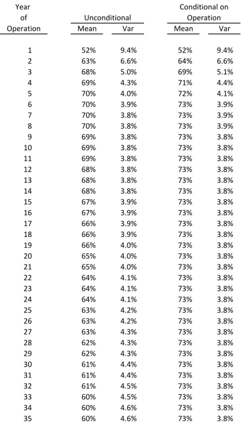
Having constructed our estimated conditional probability matrix,



, and the

probability of a permanent shutdown,



, it is straightforward to calculate the transition

matrix,



, and then the unconditional probability matrix, P. From this matrix, we can

calculate the mean load factor in each year of operation, and the variance. These are

shown in Table 8. We can also calculate a mean and variance conditional on the reactor

still being in operation, i.e., not permanently shutdown. These are also shown in Table 8.

7 _{The unconditional probability of a permanent shutdown is determined by the interaction between the}

conditional transition matrix which determines the probability of arriving at any load factor in year t-1, and this conditional probability of shutdown. Therefore, unfortunately, this scaling does not necessarily assure that the resulting unconditional probability of a shutdown matches the sample frequency. We have not estimated the discrepancy in our estimations.

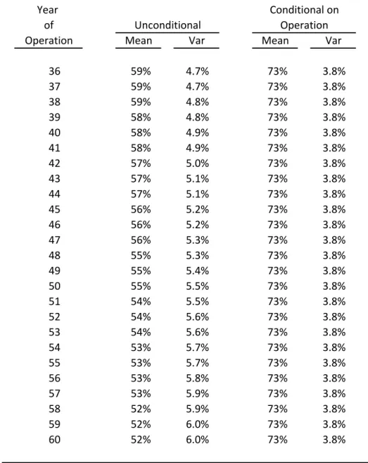
We can see from Table 8 that the conditional variance is 9.4% in the first year and

asymptotes quickly to 3.8%. The unconditional variance also is 9.4% in the first year. It

declines quickly in the next few years. Ultimately, the unconditional variance begins to

gradually rise with the year of operation, although it never reaches as high as it was in the

first year. This risk profile is the main result of this paper. It is graphed in Figure 5. The

difference between the conditional and the unconditional variance—the fact that the

unconditional variance does not asymptote, but rather begins to rise with the year of

operation—is due to the increasing cumulative probability of being permanently

shutdown in the later years of scheduled operation. We will see that this basic pattern in

both the conditional and unconditional volatility holds for all variations of the estimation

pursued later in the paper. Only the specific values change. The pattern follows from the

model of risk that we have imposed on the data.

Table 8 also shows that for the raw sample, the conditional mean capacity factor

is 52% in year 1. It quickly increases and asymptotes to 73%, which it has approximately

reached by year 6 of operation. The unconditional mean capacity factor is 52% in the first

year after start-up. The unconditional mean capacity factor also rises gradually over the

first few years of operation, reaching a peak at approximately 70%. However, it gradually

falls again to 52% by year 60 of operation. The gradual drop reflects the accreting

cumulative probability of a permanent shutdown. The increasing mean of the conditional

probability distribution in the first few years reflects the fact that the conditional

transition probability at start-up has a relatively low mean, below the steady-state

conditional distribution to which it must rise. This happens to produce the same empirical

observation as one would get with an explicit learning curve.

5. ANALYSIS AND REESTIMATION

The previous section utilized the raw PRIS data. There are several objections that

must be made to this naïve calculation.

First, the PRIS database includes several different types of reactors. The vast

majority—402 of the 535 reactors, or 75%—belong to either the boiling light water

reactor (BWR) or to the pressurized light water reactor (PWR) categories that currently

dominate the commercial reactor industry. The database also includes less popular

commercial designs such as the 53 pressurized heavy water reactors (including the

Canadian CANDUs), and designs no longer built for commercial purposes, such as the 42

gas cooled, graphite moderated reactors (widely used in the UK among other places) or

the 21 light water cooled, graphite moderated reactors (which includes the shutdown

Chernobyl reactors and cousins elsewhere in the territory of the former Soviet Union).

Being comprehensive, the database also includes unusual and experimental designs,

including 4 high temperature reactors, 4 heavy water moderated reactors, and 1 steam

generating heavy water moderated, light water cooled reactor. There are 8 fast reactors, a

very different type of reactor that has primarily been constructed on an experimental or a

demonstration basis. Does it make sense to mix the results from these different types of

reactors? Even within the two most popular categories, BWR and PWR, there are

different designs, and one could argue that the transition matrix is likely to vary across

individual reactor designs. In addition, the database includes a number of small,

experimental or demonstration reactors, and the operating experience of these will not be

comparable to that of commercial scale reactors. Lumping everything together in a single

matrix muddies the picture.

Second, the database includes reactors managed in very different types of

institutional settings. Just to illustrate, Table 3 breaks down the mean capacity factor by

reactors operated in OECD countries and reactors operated in non-OECD countries, and

there is clearly a marked difference between these two settings. Even across OECD

countries, one expects to observe different capacity factors in response to the specific

context. For example, France’s heavy reliance on nuclear power for a very large fraction

of its total electricity requirements necessarily means that some of its reactors must “load

follow”—i.e. vary their output as electricity use varies through the day, week or season.

They simply cannot all operate at a high capacity. In other countries, where nuclear

reactors represent a smaller fraction of the total generating capacity, this constraint is not

binding. Therefore, one might expect to observe a very different transition matrix for

reactors operated in France, and this would not be informative about the expected

capacity factor for a reactor being built elsewhere.

Third, the database covers a long window of time during which significant

changes occurred in reactor operations and management. We have already noted the

obvious trend in the median capacity factor apparent in Table 3. This trend may reflect a

number of different things, including changes in reactor design that make them more

reliable and easier to maintain, as well as improved management practices. For example,

in the United States, the number of days required to reload fuel fell from 104 in 1990 to

38 in 2008. This contributed significantly to raising capacity factors in the US. Given

changes such as this, to what extent is the historical data informative about future

expectations for a new reactor’s capacity factor?

Fourth, lumping all of the reactor years together into a single matrix ignores any

life-cycle pattern that may apply to the operation of a specific reactor. For example, the

literature suggests that there may be a learning curve during at least the early years of a

reactor’s operation. Although our results happen to mimic a key outcome of a learning

curve, this is not the same thing as explicitly incorporating how the transition matrix

varies with the age of the reactor. We can reorganize the PRIS data to show capacity

factors by vintage, i.e., by the year of operation of the reactor. There we see a trend

towards higher capacity factor as operating experience at the reactor increases.

The life-cycle perspective is also important as the reactor ages and reaches the

end of its anticipated useful life. Sooner or later, it will not make economic sense to

invest additional money to maintain an old reactor. In the raw database, this will show up

as a permanent shutdown. But clearly there is a difference between the events that

precipitate permanently shutting down a 40-year old reactor as scheduled, and the events

that precipitate permanently shutting down a 5-year old reactor. We should not lump both

events in the same matrix entry.

Fifth, and finally, there is some discrepancy between how we are modeling the

capacity factor and the data recorded in the PRIS database. In a financial analysis of a

new reactor build, we would like an estimate of an exogenous capacity factor variable.

This could then be combined together with estimates of the other inputs to the analysis,

such as a forecast of the electricity price, construction and operating costs, and so on, to

yield an assessment of the value of a new reactor. We could then determine how the risk

profiles of the various inputs combine together to generate a risk profile for the cash flow

and value of the reactor. What we observe in the PRIS database, however, is not a purely

exogenous variable. It is, in part, an outcome of the very valuation decision being made.

This is most obvious in the case of permanent shutdowns, as was mentioned above.

We address these five issues as follows. First, we focus our analysis on a subset of

reactors. We limit ourselves to the broad classes of BWR, PWR and PHWR designs. We

choose not to make any finer categorization so as to retain all of the information in the

combined dataset. We also excluded all reactors with capacity less than 300 MW since

most of these are either experimental or demonstration projects and not commercial

reactors. This leaves us with a total of 426 reactors.

Second, we categorize shutdowns in a manner that reflects our objective of

modeling an exogenous capacity factor variable—i.e. only premature permanent

shutdowns. Table 9a lists all reactors in our base case sample that are reported by the

PRIS database to have been permanently shutdown prior to 12/312008. We sort this list

into 2 mutually exclusive categories. One is involuntary shutdowns. This is the count that

we use to construct our premature permanent shutdown probability. The second is

voluntary shutdowns. These are excluded from the count that we use to construct our

permanent shutdown probability. The sort is done as follows. All shutdowns that occur

after the 35th year of operation are excluded from the “exogenous” shutdown category on

the basis that the plant is approximately at the end of its originally intended useful life.

We then reference the “reasons” for shutdown listed in the IAEA database. Categories

1-3 and 5-7 are counted as voluntary shutdowns and excluded from our count of premature

permanent shutdowns. Categories 4 and 8-10 are counted as involuntary shutdowns and

8 _{As we mentioned in the introduction, a few studies attempt to address this distinction explicitly, at least}

included in our count of premature permanent shutdowns. In some cases multiple reasons

are given: whenever at least one reason falls in the involuntary category, the reactor is

categorized as involuntarily shutdown and added to our premature permanent shutdown

count. At the conclusion of this step we are left with 13 reactors in our base case sample

that were involuntarily shutdown and that enter into our count as premature permanent

shutdowns.

Table 9b lists all reactors in our base case sample that are reported by the PRIS

database to have experienced an extended period of dormancy, i.e., 4 or more years with

no commercial production. These are reactors that are shutdown for an extended period

of time, but continue on the IAEA’s list as still licensed for operation. In 11 cases

identified in the table we treat these reactors as having been permanently shutdown at the

start of the dormancy period. According to our algorithm stated above, these shutdowns

are treated as voluntary and therefore do not add to the permanent shutdown count. If the

reactor was extensively rebuilt prior to restart of operation or if the reactor enters final

shutdown during its dormancy, the later years of zero production are not used in the

counts creating our conditional transition matrix. In four cases identified in the table,

after substantive reinvestment and new construction, the reactor is re-started, and we treat

this as an entirely new reactor.

We believe this methodology is likely to underestimate the sample frequency of

premature permanent shutdowns caused by exogenous factors, at least as a financial

investor considering the value of constructing a new reactor is likely to view it. Several of

the shutdowns that are categorized as voluntary could easily be categorized as

involuntary, once again from the perspective of the financial investor: for example, the

shutdown of the Browns Ferry reactors in the US, the shutdown of the Armenia reactor,

and the shutdown of the Barsebäck reactor in Switzerland, to name a few. And some

reactors that began construction but were never completed or that never generated power

commercially—such as the Shoreham plant in the US—never make it into the dataset and

so do not add to the count of permanent shutdowns.

Because even a small number of permanent shutdowns has a large impact on the

unconditional expected capacity factor, and because of the subjective element involved in

assessing the relevance of the small sample of permanent shutdowns for future operation,

the correct estimation of the probability of a permanent shutdown going forward is likely

a very contentious issue in valuation of a new nuclear power plant. The algorithm chosen

here results in a much smaller count of prematurely permanently shutdown reactors than

in the raw dataset. This has a major effect on the unconditional expected capacity factor

and on the unconditional volatility of the capacity factor, as we shall see below. This

emphasizes the necessity of applying careful judgment in estimating this probability

using historical data.

After taking these two steps, we have what we call our complete “base case” data.

We use this data to reproduce the transition matrix calculations and we report those

results below.

We then do 3 subsidiary analyses. First, we produce transition matrix calculations

broken down by bloc—OECD vs. non-OECD. Second, we produce transition matrix

calculations broken down by reactor age. We group the reactors years into the first 5

years of operation and the remaining years. Third, and finally, we produce transition

matrix calculations broken down by epoch—before and after 2000. These three analyses

are not statistically independent of one another. For example, non-OECD reactor year

observations are more heavily concentrated in the post-2000 data set. The post-2000 data

set contains a different profile of observations at the different age in a reactor’s life as

compared to the pre-2000 data set. These 3 analyses do not generate statistical tests of the

differences, but merely identify the size of the differences one finds in the data set.

Obviously, finer breakdowns lead to even sharper distinctions. To illustrate, we report

results for the post-2000 data for three specific countries: the US, France and Japan.

Base Case Results

Table 10 shows the estimation of the parameters of the conditional probability

distributions for the conditional transition matrix,



, using the base case data. Table 11

shows the estimation of the probabilities of permanent shutdown,



. Table 12 shows the

mean and variance from the unconditional transition matrix, P, through the life of the

reactor.

From Table 12, we see that the conditional variance is 9.5% in the first year of

operation. It quickly asymptotes to 3%. The unconditional variance is also 9.5% in the

first year. It then falls to 2.9%. Unlike in the raw data case, there is no discernable

increase in the unconditional volatility. This is due to the low probability of a permanent

shutdown in our base case.

We also see from Table 12 that conditional mean capacity factor starts at 53.5%

and quickly increases to the asymptote of 74.5%. The uncondititional mean capacity

factor starts out at 53.5%. It quickly climbs towards its peak of just over 74%. The peak

is reached in year 7. After this the unconditional probability declines, but only very

gradually, so that the expected capacity factor is only slightly below 73% at the end of 40

years and just below 72% at the end of 60 years.

Bloc results

The base case dataset is further divided into an OECD dataset and a non-OECD

dataset. There are 428 OECD reactors and only 107 non-OECD reactors in the raw PRIS

database, and 353 OECD reactors (360 counting the rehabilitated units) and only 72

non-OECD reactors in the base case database. Tables 13-15 show the results for the non-OECD,

while Tables 16-18 show the results for the non-OECD. Comparing the unconditional

mean capacity factors calculated from the P matrices reported in Tables 15 and 18 we see

that the mean capacity factor in OECD reactors is higher than non-OECD reactors. For

example, at year 10 the OECD mean capacity factor is 75.2% versus 64.8% in the

non-OECD. This is a result of differences in both the conditional probability matrix,



, and

the probability of permanent shutdowns,



. Some of the differences in the conditional

probability matrix can be summarized in the steady-state mean conditional capacity

factors reported in Tables 15 and 18. The steady-state mean conditional capacity factor in

OECD reactors is higher than non-OECD reactors, 75.3% versus 69.2%. The probability

of a shutdown is lower among OECD reactors than among non-OECD reactors.

Interestingly, a comparison of Tables 15 and 18 reveals that the variance of the

capacity factor is greater when constructed from the OECD reactor data than when

constructed from the non-OECD reactor data. For example, in the second year of

operation, the unconditional variance in the OECD capacity factor is 5.2% versus 3.5%

for the non-OECD capacity factor. The variance of the steady-state conditional

distribution for the OECD capacity factor is 3% versus 1.9% for the non-OECD capacity

factor.

Epoch results

The base case dataset is divided into transitions occurring pre- and post-2000.

Transitions from 1999 into 2000 are assigned to the post-2000 dataset. Tables 19-21

show the results constructed using the pre-2000 experience, while Tables 22-24 show the

results constructed using the post-2000 experience. Comparing the unconditional mean

capacity factors calculated from the P matrices reported in Tables 21 and 24 we see that

the mean capacity factor 2000 is lower than post-2000 reactors. At year 10 the

pre-2000 mean capacity factor is 70.9% versus 77.8% post-pre-2000. This is a result of

differences in both the conditional probability matrix,



, and the probability of

permanent shutdowns,



. As one can see in Tables 21 and 24, the steady-state mean

conditional capacity factor in pre-2000 reactors is lower than post-2000 reactors, 71.5%

versus 78.2%. The probability of shutdowns is greater among reactors pre-2000 than

post-2000.

A comparison of Tables 21 and 24 reveals that the variance of the capacity factor

is greater when constructed from the pre-2000 data than when constructed from the

post-2000 data. For example, in the second year of operation, the unconditional variance

constructed using the pre-2000 data is 4.8% versus 3.6% using the post-2000 data. The

variance of the steady-state conditional distribution from the pre-2000 data is 2.9%

versus 2.1% for the post-2000 data.

Age results

The base case dataset is divided into transitions occurring during the first 5 years

of operation and transitions occurring after the first 5 years of operation. Transitions from

year 4 into year 5 are in the first category, and transitions from year 5 into year 6 are in

the second category. Tables 25 and 26 show the estimation of the parameters of the

conditional probability distributions for the conditional transition matrix,



, and the

estimation of the probabilities of permanent shutdown,



, using the experience from

the first 5 years of operation. These matrices include the start-up probability distribution.

Tables 27 and 28 shows the corresponding estimates,



and



, using the

experience from the years of operation after the first 5 years of operation. These matrices,

of course, do not include a start-up probability distribution. Table 29 shows the mean and

variance from the unconditional transition matrix, P, through the life of the reactor

constructed using



and



to generate the probabilities over the first 5 years of

operation and



and



, to generate the probabilities for the remaining years.

Comparisons of Tables 25 and 27 show that differences in the conditional

probability matrix,



, do not yield an unambiguous comparison of mean conditional

capacity factors independent of the prior year’s capacity factor. When the prior year’s

capacity factor is high, reactors with more than 5-years operating experience have a

higher conditional mean operating factor than do reactors with less than 5-years operating

experience. However, when the prior year’s capacity factor is low, reactors with more

than 5-years operating experience have a lower conditional mean operating factor than do

reactors with less than 5-years operating experience. This would make sense if, for

example, a low capacity factor in the early years reflected, in part, shake-out problems

that can occur at the start-up of any reactor, while a low capacity factor in later years

more purely reflected reactor specific problems that persist across years.

The sample frequency of permanent shutdowns is concentrated in the early years

of operation.

A comparison of Table 29 against Table 12 shows that segmenting the data set by

age of operation produces a slightly lower mean capacity factor in the early years of

operation, and a slightly higher mean capacity factor in the later years. In year 2, the

unconditional mean load factor is 66.1%, very slightly below the 67.1% unsegmented

base case result. By year 10, the unconditional mean load factor is 74.3%, very slightly

above the 74% unsegmented base case result. The steady-state conditional load factor is

75.1% in the segmented data, as opposed to 74.5% in the unsegmented base case results.

Interestingly, segmenting by age lowers the volatility of the unconditional

distribution in the first years of operation as can also be seen in a comparison of Tables

29 and 12. For example, shows that the unconditional variance in year 2 constructed

using age segmented data is 3.8% versus 5.2% in the base case. The variance of the

steady-state conditional distribution from the age segmented data is by construction

identical to the figure for the base case, 3.1%.

Country specific results

The relatively low mean capacity factors reported above for the OECD and for

post-2000 data are surprising to some. This is especially true for those who have given

attention to the very high capacity factors attained in the United States in recent years.

The explanation is to be found in the fact that country specific results are highly variable.

For example, in this period when the US began to attain very high capacity factors, Japan

confronted major problems at a number of reactors, lowering the average in Japan

dramatically. Persons focusing on one country will arrive at starkly different estimates

depending upon which is chosen. Our results above average across these individual

country samples. Also, as mentioned in the opening discussion about capacity factors, the

situations vary across countries, and France, in particular, runs a number of reactors to

follow load and so has lower capacity factors.

To see this, we report results for these three countries estimated separately using

post-2000 data. Tables 30-31 report results for the US, Tables 32-33 report results for

Japan, and Tables 34-35 report results for France. In each case, we report the parameters

of the Conditional Transition Probability matrix,



, calculated using post-2000 data.

Since none of the countries had any of what we classify as involuntary permanent

shutdowns during this period, we only report the distribution moments for the load factor,

conditional on continuing operation, from P. Also, due to the small number of reactor

starts—none in some cases—we employ the conditional probability vector for a start-up

reactor calculated from the full OECD data.

Obviously, when one repeats the analysis for finer subsets of the data one obtains

more variable results as one can see by comparing the starkly different mean capacity

factors for these three countries using the post-2000 dataset. Table 31 shows that the

steady-state mean conditional capacity factor in the US post-2000 is 92.7%. Table 33

shows that the same parameter for Japan is only 66.7%, while Table 34 shows that it is

75.2% for France.

The variance of the steady-state conditional distributions are also different,

although the time pattern is similar. For the US the variance of the steady-state

conditional distribution is 0.4%, for Japan it is 2.9% and for France is is 0.5%.

The contrasts across these countries makes clear how large a role judgement must

play in making use of the available data. Obviously, if one wants to forecast the capacity

factor risk structure in the US, it may make good sense to set aside or otherwise minimize

the French data since one knows a priori that the institutional settings are starkly different

and this may be the major factor in the different mean capacity factors. However, setting

aside the Japanese data is more troublesome. One can make an argument that Japanese

specific geography—vulnerability to earthquakes—as well as country specific corporate

and regulatory failures are the reasons for the low capacity factors, and that these do not

apply to the US. However, the fact that in an earlier era it was the US that saw very low

capacity factors due to country specific corporate and regulatory failures, makes this a

weaker position. The current Japanese experience and the earlier US experience could

reflect a common underlying vulnerability for this complicated technology, one that

could show-up in any country in the future, always in the guise of country specific

circumstances. It is not our objective here to resolve this issue, but only to highlight the

significant judgment that must be applied in deciding which data to rely upon for making

future projections.

5. CONCLUSIONS

We developed a fully specified model of the dynamic structure of capacity factor

risk. It incorporates the risk that the capacity factor may vary widely from year-to-year,

and also the risk that the reactor may be permanently shutdown prior to its anticipated

useful life. We then fit the parameters of the model to the IAEA’s PRIS dataset of

historical capacity factors on reactors across the globe.

Our main result is that capacity factor risk is greatest in the first year of operation,

declining quickly over the next couple of years, after which it is approximately constant

or gradually increasing. Whether risk is constant or increasing in later years depends

significantly on the probability of an early, permanent shutdown of the reactor. Our base

case is parameterized with a conservatively low probability of a permanent shutdown

which yields approximately constant variance after the first few years.

Although our original objective was to understand the dynamic structure of

capacity factor risk, in estimating our model we also found interesting results about the

expected level of the capacity factor. Our model, combined with the global historical

dataset, yields relatively low estimates for the expected level of the capacity factor

through the life of the plant. Our base case estimate is approximately 74%. If we

construct our estimate using historical data only for reactors installed in OECD countries,

the estimate improves by approximately 1 percentage point. If we construct our estimate

using historical data only for reactor performance since the year 2000, the estimate

improves by approximately 4 percentage points. If we construct our estimate recognizing

the different performance characteristics of young and old reactors, the estimated mean

capacity factor is reduced in the first few years of operation, and increased in the later

years. In this preliminary analysis, we did not attempt to construct an estimate combining

each of these effects. But it is difficult to see from this first pass through the data how

that would likely yield a result at all close to the 85% or 90% figures that are commonly

used in advocating construction of new nuclear power plants.

Justification for such a high estimated mean capacity factor appears to require

focusing exclusively on a much smaller subset of the data—e.g. only at the performance

of mature plants in the United States since the year 2000—and simultaneously ignoring

all of the other available data and experience. Certainly there may be a good reason for

focusing on a small subset of the data and ignoring the other data. It is equally wrong to

naively treat all datapoints as equally informative as it is to naively focus on only some of

the datapoints and ignore the others. But we have not seen a careful justification for high

estimates of the mean capacity factor that seriously confront the potential information

available in the full data set.

We should reiterate here that we have been very conservative in calculating our

estimate of the probability of a permanent shutdown. Our estimates using the raw data set

show that a higher probability of a permanent shutdown could be easily rationalized

using the historical experience. This parameter has a very strong influence on the

unconditional mean capacity factor. Here again, judgment in exploiting the historical data

is key. We obtain our low estimate of the unconditional mean capacity factor despite

being very conservative in estimating the probability of a permanent shutdown.

REFERENCES

David, Paul A, Roland Maude-Griffin, and Geoffrey Rothwell, 1996, Learning by

Accident? Reductions in the Risk of Unplanned Outages in U.S. Nuclear Power

Plants After Three Mile Island, Journal of Risk and Uncertainty, 13, 175-198.

Easterling, Robert G., 1982, Statistical Analysis of U.S. Power Plant Capacity Factors

through 1979, Energy, 7.3, 253-258.

Hultman, Nathan E., Jonathan G. Koomey, and Daniel M. Kammen, 1 April 2007, What

History Can Teach Us about the Future Costs of U.S. Nuclear Power,

Environmental Science and Technology, 2088-2093.

Joskow, Paul L. and George A. Rozanski, 1979, The Effects of Learning by Doing on

Nuclear Plant Operating Reliability, The Review of Economics and Statistics,

61.2, 161-168.

Komanoff, Charles, 1981, Power Plant Cost Escalation: Nuclear and Coal Capital Costs,

Regulations, and Economics, New York: Van Nostrand Reinhold Company.

Koomey, Jonathan and Nathan E. Hultman, 2007, A reactor-level analysis of busbar costs

for US nuclear plants, 1970-2005, Energy Policy, 35, 5630-5642.

Krautmann, Anthony C. and John L. Solow, 1988, Economies of Scale in Nuclear Power

Generation, Southern Economic Journal, 55.1, 70-85.

Lester, Richard K. and Mark J. McCabe, 1993, The Effect of Industrial Structure on

Learning by Doing in Nuclear Power Plant Operation, The RAND Journal of

Economics, 24.3, 418-438.

Rothwell, Geoffrey, 1990, Utilization and Service: Decomposing Nuclear Reactor

Capacity Factors, Resources and Energy, 12, 215-229.

---, 1996, Organizational Structure and Expected Output at Nuclear Power Plants, The

Review of Economics and Statistics, 78.3, 482-488.

---, 2006. “A Real Options Approach to Evaluating New Nuclear Power Plants,” The

Energy Journal 27, 1.

Rothwell, Geoffrey and John Rust, 1995, A dynamic programming model of US nuclear

power plant operations, University of Wisconsin Department of Economics.

---, 1995, Optimal Response to a Shift in Regulatory Regimes, Journal of Applied

---, 1997, On the Optimal Lifetime of Nuclear Power Plants, Journal of Business and

Economic Statistics, 15.2, 195-208.

Samis, Michael, 2009, Using Dynamic Discounted Cash Flow and Real Option

Simulation to Analyze a Financing Proposal for a Nuclear Power Plant, Ernst &

Young presentation.

Sturm, Roland, 1993, Nuclear power in Eastern Europe: Learning or forgetting curves?,

Energy Economics, 15.3, 183-189.

---, 1994, Proportional hazard regression models for point processes: An analysis of

nuclear power plant operations in Europe, Journal of Applied Statistics, 21.6,

533-540.

---, 1995, Why does nuclear power performance differ across Europe?, European

Economic Review, 39.6, 1197-1214.

100 94 88 82 76 70 64 58 52 46 40 34 28 22 16 10 4 100 91 82 73 64 55 46 37 28 19 10 1 0 0.1 0.2 0.3 0.4 0.5 0.6 Probability  of  transition LF in year n+1 LF in year n

Figure 1

Transition Matrix from Raw PRIS Database

Figure 2

Sample and Fitted Mean of the Conditional Transition Probabilities

0% 10% 20% 30% 40% 50% 60% 70% 80% 90% 100% 0 10 20 30 40 50 60 70 80 90 100

Load Factor in Year n

Figure 3

Sample and Fitted Variance of the Conditional Transition Probabilities

12% 14% 10% 6% 8% Variance 4% 0% 2% 0 10 20 30 40 50 60 70 80 90 100