HAL Id: hal-00646123
https://hal.inria.fr/hal-00646123
Submitted on 29 Nov 2011
HAL is a multi-disciplinary open access
archive for the deposit and dissemination of sci-entific research documents, whether they are pub-lished or not. The documents may come from
L’archive ouverte pluridisciplinaire HAL, est destinée au dépôt et à la diffusion de documents scientifiques de niveau recherche, publiés ou non, émanant des établissements d’enseignement et de
Order statistics and estimating cardinalities of massive
data sets
Frédéric Giroire
To cite this version:
Frédéric Giroire. Order statistics and estimating cardinalities of massive data sets. Discrete Applied Mathematics, Elsevier, 2009, 157 (2), pp.406-427. �hal-00646123�
Order Statistics and Estimating Cardinalities
of massive Data Sets
Fr´ed´eric Giroire
1ALGO project, INRIA Rocquencourt, B. P. 105, 78153 Le Chesnay Cedex, France; and MASCOTTE, joint project CNRS-INRIA-UNSA, 2004 Routes des Lucioles,
BP 93, F-06902, France.
Abstract
A new class of algorithms to estimate the cardinality of very large multisets using constant memory and doing only one pass on the data is introduced here. It is based on order statistics rather than on bit patterns in binary representations of numbers. Three families of estimators are analyzed. They attain a standard error of √1
M using M units of storage, which places them in the same class as the best known algorithms so far. The algorithms have a very simple internal loop, which gives them an advantage in term of processing speed. For instance, a memory of only 12kB and only few seconds are sufficient to process a multiset with several million elements and to build an estimate with accuracy of order 2 percents. The algorithms are validated both by mathematical analysis and by experimentations on real internet traffic.
Key words: cardinality, estimates, very large multiset, traffic analysis
1 Introduction
Problem. A multiset is a set where each element can appear several times. The cardinality n of the multiset is the number of distinct elements, while the size N of the multiset is the total number of elements, counting the repeti-tions. An important issue in computer science is to estimate the cardinality of a multiset having a very large size. This problem has arisen in the 1980’s, motivated by optimisations of classical algorithmic operations on data bases
Email address: [email protected](Fr´ed´eric Giroire). URL: http://algo.inria.fr/giroire/(Fr´ed´eric Giroire). 1 Partially supported by the European FET project AEOLUS.
(union, intersection, sorting,...). As the data sets to be measured have mostly a very large size N, far beyond the RAM capacities, a natural requirement is to treat the data in one pass using a simple loop, and with a small auxiliary memory (constant or logarithmic in N). More recently, in the past decade, the problem of counting distinct elements has appeared as a crucial algorithmic operation in the context of networking with the development of networks of very large capacity. Typically, the elements are packets, each packet belonging to a flow (also called connection) identified by a source address and a des-tination address. Estimating the number of distinct flows in a data stream has many applications in network monitoring and network security, see the detailed survey of Estan, Varghese and Fisk [7]. For instance, one can count the number of distinct flows on a traffic to detect Denial of Service attacks, where abnormally many distinct connections are opened in a short period of time. Other applications include the data mining of language texts [2, 3] or biological data [16, 17]. The crucial point to solve the problem, first developed by Flajolet and Martin [10] in their algorithm Probabilistic Counting, is to relax the constraint of giving the exact number of distinct values in the mul-tiset. For most applications, a probabilistic estimate of n with good precision is sufficient.
The three families of algorithms. In this article, new estimators, based on order statistics, are introduced to solve the problem of estimating the car-dinality of very large multiset while using constant memory and performing a single pass on the data. In addition, no assumption is made on the structure of the data.
We assume that a hash function h mapping an element to a real value that “looks like” uniformly distributed in the interval [0, 1] is given (see the detailed study of Knuth [19]). Let S = (e1, . . . , eN) be a set of elements and let n be the
number of distinct elements in S. Under the assumption on the hashed function h, and without making any assumption on the nature of the repetitions, the set (h(e1), . . . , h(eN)) of hashed values can be considered as built from n real
values taken independently uniformly at random in [0, 1], and then replicated and permuted in an arbitrary way. Such a set of uniform random values in [0, 1] with arbitrary replications and order of appearance is called an ideal multiset. Thus, estimating the number of distinct elements in a real multiset without making any assumptions on the repetitions amounts to estimating the cardinality of an ideal multiset.
The crucial idea is then that the minimum value in an ideal multiset does not depend on the replication structure of the data nor on the ordering, and gives an indication on the number n of distinct values of the multiset (basically, the minimum of n independent uniform values on [0, 1] has more chances of being small if n is large). More precisely, the expectation of the minimum is
1
this minimum, but the inverse happens to have an infinite expectation. To overcome this difficulty, our solution is to build estimates using the inverse of the k-th minimum —instead of the first minimum— composed with a sublinear function, as logarithm or square root. It gives three families of estimates of n: the Inverse, Logarithm and Square Root Families. The estimates are then combined with a stochastic averaging process, as introduced by Flajolet and Martin in [10]. Stochastic averaging consists in simulating the effect of m experiments on the multiset and then averaging an observable over the m experiments to obtain an estimate with a good precision.
Related work. There has been substantial work on approximate query pro-cessing in the database community, see [14, 13, 5]. In [20] Whang, Zanden and Taylor introduced Linear Counting. The principle is to distribute hashed values into buckets and use the number of hit buckets to give an estimate of the number of values. A drawback of this method is that memory is still linear (but with a small constant). To extend it to very large data sets, Es-tan, Varghese and Fisk proposed in [7] a multiscale version of this principle in their Multiresolution Bitmap algorithm. The algorithm keeps a collec-tion of windows on the previous bitmap. Its estimate has a standard error of 4.4/√m while using m words of memory. Another way that has been proposed to estimate cardinality is sampling. The idea is to keep only a fraction of the values that have been read. For instance, in Wegner’s Adaptive Sampling this fraction is dynamically chosen in an elegant way. The algorithm has been described and analyzed by Flajolet in [8] and its accuracy is 1.20/√m. The Probabilistic Counting algorithm of Flajolet and Martin, in [10], uses bit patterns in binary representations of numbers. It has excellent statistical properties with an error close to 0.78/√m. In [6], the LogLog Counting al-gorithm of Durand and Flajolet starts from the same idea but uses a different observable. The standard error is 1.30/√m, but the m words of memory have here a size of order log log n and not log n. The same is true for the algorithm HyperLogLog, introduced in [9], based on the harmonic mean rather than the geometric mean, which attains a precision of 1.04/√m, giving it the best known ratio precision over memory. Finally in [1] the authors present three algorithms to count distinct elements. The first one uses the k-th minimum and corresponds basically to the inverse family estimator. The authors prove that this algorithm (!, δ)−approximates n using O(1/!2log m log(1/δ)) bits of
memory and O(log(1/!) log m log(1/δ)) processing time per elements. In this paper, we generalize this idea by introducing new and more efficient families of estimates and provide a precise analysis. A short version of this work can be found in [15]. Finally, in [4], Chassaing and Gerin propose an other family of estimators and prove its optimality using information and estimation theory. Results. The three families of estimators are presented in Section 2 and an-alyzed in Section 4. The main results are presented before the analysis in Section 3. We found asymptotically unbiased estimates of n for the three
fami-lies and give their standard error in Theorem 1. We then compare the tradeoffs between accuracy and memory requirement for these families in Theorem 2. We show that, with a fixed amount of memory, M, the precision improves when k increases and that better estimates are obtained when applying sub-linear functions. Nevertheless, the three families have an optimal trade-off of 1/√M. In addition, we propose a best practical estimate, Mincount. Using an auxiliary memory of only 12kB, it succeeds in estimating with accuracy of order 2 percents the cardinality of a multiset with several million elements. Note that the algorithms can be adapted to operate on sliding windows [12]. Validation and experimentations. The estimates of the three families are validated using trace files of different kinds (e.g. english texts or router traces) and sizes. The relative error of the estimates is shown to be close to what expected from theory (see Figure 4 in Section 5). We also show that the al-gorithms are very fast: our implementation takes only few seconds to process files with millions of elements and is only 3 to 4 times slower than the very simple unix command cat -T, that just replaces the tab characters of a file by ˆI (see Figure 6). This is of critical value in the context of in-line analysis of internet traffic where we have only of few tens of machine operations at disposal to process a packet. In Section 5.4, we show how the algorithm Min-count can be used to detect some attacks on a network, e.g. the spreading of the worm Code Red.
2 Three families of estimates
In this section, we present three families of algorithms, the Inverse, Square Root and Logarithm Families, to estimate the cardinality of very large multi-sets.
Construction of estimators based on the minimum M. Recall from the previous section that we assume at our disposal a hash function h mapping any element to a real value that “looks like” uniformly distributed in the in-terval [0, 1] —the construction of this hash function may be based on modular arithmetic as discussed by Knuth in [19]. Given any multiset, we can transform it to an ideal multiset (defined previously) by using such a hash function on the elements in the multiset. Thus, the problem of estimating distinct items in a multiset is equivalent to estimating the cardinality of an ideal multiset. To estimate the number of distinct elements, denoted by n, of an ideal multiset, we consider its minimum, M. An important remark is that the minimum of a sequence of numbers is found with a single pass on the elements and that it is not sensitive to repetitions. The density of the minimum of n uniform random variables over [0, 1] is P(M ∈ [x, x + dx]) = n(1 − x)n−1dx. So, for n ≥ 1, its
expectation is E[M] = ! 1 0 x · n(1 − x) n−1dx = 1 n + 1.
M is roughly an estimator of 1/n. Our hope is now to be allowed to take 1/M as an estimate of n. But E " 1 M # = ! 1 0 1 x · n(1 − x) n−1dx = +∞
Unfortunately, the integral does not converge near 0 and is unbounded. In order to obtain an estimate of n we use indirectly the minimum M in the following ways.
(1) Instead of using the inverse function alone, we compose it with a sublinear function f , e.g. the (natural) logarithm and the square root.
(2) Instead of using the first minimum, we take the second, third or more generally the k-th minima.
Thus we obtain three families of estimates namely the Inverse Family, the Square Root Family and the Logarithm Family. We talk about families as we have one estimator per value of k. Their pseudo-code is given in Figure 1. Simulating m experiments. The precision of the algorithms is given by the standard error of their estimate ξ, denoted by SE[ξ] and defined as follows
SE[ξ] := σ(ξ) n ,
where σ(ξ) denotes the standard deviation of ξ. To improve the precision of the algorithms, we would like to average over several similar experiments, as it is well known that the arithmetic mean of m i.i.d. random variables with expectation µ and standard deviation σ has same expectation µ but a standard deviation scaled down by 1/√m. Doing m experiments involves using m different hashing functions. But hashing all the elements m times is particularly time consuming and building m independent hashing functions is not an easy task. To avoid these difficulties we use a stochastic averaging process, as introduced by Flajolet and Martin in [10]. Stochastic averaging consists in simulating the effect of m experiments on the multiset while using a single hash function and then averaging an observable over the m experiments. The principle is to distribute the hashed values among m different buckets. That is done by dividing [0, 1] into m intervals of size 1/m. A hashed value x falls in the i-th bucket if i−1m ≤ x < mi . Our algorithms keep the k-th minimum of the i-th bucket, denoted by Mi(k) in the analysis, for i from 1 to m (note that the Mi(k) have to be rescaled by M
(k)
i ← m · (M
(k)
i − i−1m ) to produce
elements in the unit interval). A precise estimate is then built by averaging estimates built from the minimum of each bucket, as seen in Section 3.
Inverse Family Algorithm (F : multiset of hashed values; m) for x ∈ F do
if i−1m ≤ x ≤ mi do
actualize the k minima of the bucket i with x return ξ1 := (k − 1)$mi=1M1(k)
i
as cardinality estimate.
Square Root Family Algorithm (F : multiset of hashed values; m) for x ∈ F do
if i−1
m ≤ x ≤
i m do
actualize the k minima of the bucket i with x
return ξ2 := % 1 1 (k−1)+(k−1)!2m−1 Γ(k− 1 2)2 & $m i=1)1 Mi(k) 2 as cardinality estimate.
Logarithm Family Algorithm (F : multiset of hashed values; m) for x ∈ F do
if i−1m ≤ x ≤ mi do
actualize the k minima of the bucket i with x return ξ3 := m · , Γ(k−1 m) Γ(k) -−m · e−m1 $m i=1ln M (k) i as cardinality estimate.
Fig. 1. Pseudo-code of the three families of estimates.
3 Results of the analysis of the three families of estimates.
The main results of the analysis are presented here. The analysis itself and all the proofs can be found in Section 4. We found asymptotically unbiased estimates of n for the three families and give their standard error in Theorem 1. Note that all results for the Inverse and the Square Root family are given for k ≥ 3.
Theorem 1 Consider the algorithms of the three families built on the k-th minimum (k ≥ 3) using a stochastic averaging process simulating m experi-ments and applied to an ideal multiset of unknown cardinality n.
(1) The estimates returned by the Inverse Family, ξ1, the Square Root Family,
ξ1:= (k − 1) m . i=1 1 Mi(k), ξ2:= 1 % 1 k−1 +(k−1)!m−12Γ(k − 12)2 & m . i=1 1 ) Mi(k) 2 and ξ3:= m · / Γ(k − 1 m) Γ(k) 0−m · e−m1 $m i=1ln M (k) i ,
are asymptotically unbiased in the sense that, for i = 1, 2, 3 E[ξi] ∼
n→∞n.
(2) Their standard error, defined as 1 n ) V(ξi), satisfies SE[ξ1] ∼ n→∞C1(m, k) := 1 √ k − 2 · 1 √ m, SE[ξ2] ∼ n→∞C2(m, k) := 1 m2 / 1 k − 1 + (m − 1)Γ(k − 12)2 (k − 1)!2 0−2 · m (k − 1)(k − 2) + 8%m2&Γ(k − 32)Γ(k − 12) (k − 1)!2 + 6 %m 2 & (k − 1)2 + 36%m3&Γ(k − 12)2 (k − 1)(k − 1)!2 + 24%m4&Γ(k − 12)4 (k − 1)!4 − 1 1/2 , SE[ξ3] ∼ n→∞C3(m, k) := 5 6 6 7 / Γ(k − 1 m) Γ(k) 0−2m · / Γ(k − 2 m) Γ(k) 0m − 1, where Γ is the Euler Gamma function defined in Section 4.1.
Note that the equivalents of the standard errors —C1(m, k), C2(m, k) and
C3(m, k)— do not depend on n. They are studied for m large in Lemma 1
—the proof is given in Section 4.6.
Lemma 1 When m large, the equivalents of the standard errors of the esti-mates of the three families, C1(m, k), C2(m, k) and C3(m, k), defined in
The-orem 1, are equivalent to
C1(m, k) ∼ m→∞ 1 √ k − 2 · 1 √ m, C2(m, k) ∼ m→∞2 · 5 6 6 7 1 k − 1 / Γ(k) Γ(k − 1 2) 02 − 1 ·√1 m, C3(m, k) ∼ m→∞ ) ψ%(k) ·√1 m,
where Γ and ψ% are the Euler Gamma and Trigamma functions defined in
Section 4.1.
We now want to compare the algorithms when m is large (we want precise estimates) with respect to the trade-off between precision and memory. The memory used by the algorithms is that required to store the minimums, i.e., km floating numbers for an estimate built with the k-th minimum. The metric here is the precision defined as the relative error of the estimates expressed as a function of the memory, noted M (= km). We have
Theorem 2 (Precision of the algorithms) The precision of the three fam-ilies of estimates, P1(M, k), P2(M, k) and P3(M, k), given by
P1(M, k) := 8 k k − 2 · 1 √ M, P2(M, k) := 2 · 5 6 6 6 7k 1 k − 1 / Γ(k) Γ(k − 1 2) 02 − 1 · 1 √ M, P3(M, k) := ) k · ψ%(k) · √1 M, satisfy, for a fixed M,
(1) P1(M, k), P2(M, k) and P3(M, k) are decreasing functions of k;
(2) when k is large, for i = 1, 2, 3,
Pi(M, k) → k→∞
1 √
M.
The proof is given in Section 4.7. The precisions of the three families can be written Pi(M, k) = Ci(k) · √1M, for i = 1, 2, 3. Note that Ci(k) does not
depend on M. Figure 2 gives these constants for different values of k. Four main results can be extracted from the theorem.
First result. As expressed in (1), for the three families, the precision improves as k increases. For example, for the logarithm family, we have P3(M, 1) =
1.28/√M , P3(M, 2) = 1.14/
√
M and P3(M, 3) = 1.09/
√ M .
Second result. As expressed in (2), there exists an optimal trade-off between precision and memory for the three families: a precision of 1/√M using a memory of M floating numbers.
For practical purposes, we compare the constants of the precision of the three families of estimate and choose a best practical estimate.
20 2 0 1 1.5 10 5 15 k Inverse Family Square Root Family Logarithm Family Precision k C1(k) C2(k) C3(k) 1 − − 1.28 2 − − 1.14 3 1.73 1.26 1.09 5 1.29 1.13 1.05 10 1.12 1.06 1.03 100 1.01 1.006 1.003
Fig. 2. Constants of the precision of the three families of estimates for different values of k.
Third result. Though the three families have the same asymptotical preci-sion, we observe that, for all reasonable practical values of k, the precision of the estimate of the Logarithm Family is better than the precision of the estimate of the Square Root Family which is better than the one of the Inverse Family (see Figure 2), that is, for all 3 ≤ k ≤ 1000,
P1(M, k) ≥ P2(M, k) ≥ P3(M, k).
For example, in the case of the third minimum, we have P1(M, 3) = 1.73/
√ M , P2(M, 3) = 1.26/ √ M and P3(M, 3) = 1.09/ √
M . More values can be found in Table 1. It means that better estimates are obtained when we apply sublinear functions, such as square root or logarithm.
Fourth result: Best practical estimate. In practice, the optimal efficiency is reached quickly. As a matter of fact, the constant for the estimate of the Logarithm Family using only the third minimum is 1.09. We consider this estimate as the best practical estimate. An optimized implementation of an algorithm using this estimate, Mincount, is used in Section 5.3 to study the execution times and in Section 5.4 to analyze Internet traffic traces. Note that, as the best efficiency is attained quickly, the introduction of other families of estimates built with “more” sublinear functions, e.g. ln2, would not provide enough practical gains in terms of precision.
4 Analysis of the three families of estimates.
The proofs of the results enounced in Section 3 are given here. The main part of this section is the proof of Theorem 1 which shows that the estimates are asymptotically unbiased and gives their standard error. The steps of the analysis are presented in Section 4.2. The proof is then given in Section 4.3 for
the Inverse Family, in Section 4.4 for the Logarithm Family and in Section 4.5 the Square Root Family. The computations strongly rely on special functions; classical definitions and results are first recalled in Section 4.1. The section ends with the proofs of Lemma 1 (analysis of the standard error for large m) and Theorem 2 (comparison of the precision of the estimates) in Sections 4.6 and 4.7.
4.1 Preliminaries: special functions
The computations of the expectations and the standard errors of the esti-mates intensively use some special functions, in particular the Euler Gamma function, defined as
Γ(z) :=
! ∞
0 t
z−1e−tdt,
and the Euler Beta function, defined as B(α, β) :=
! 1
0 t
α−1(1 − t)β−1dt.
These two functions and their derivatives are intimately related as B(α, β) = Γ(α)Γ(β)Γ(α + β)
and
d
dαB(α, β) = B(α, β)(ψ(α) − ψ(α + β)),
where ψ is the logarithmic derivative of the Gamma function, also called Digamma function. This last function is defined as
ψ(z) = d
dz ln Γ(z) = Γ%(z)
Γ(z).
The Digamma function ψ is related to the Harmonic Sum Hn:=$nk=1k1 by
ψ(n) = Hn−1− γ,
where γ is the Euler constant defined as limn→∞(Hn− ln n).
The derivative of the function ψ, denoted by ψ%, is called Trigamma function
and is also used in this paper. One of its interesting property is that ψ%(z) = ∞ . k=0 1 (z + k)2.
4.2 Method of analysis
Recall that the stochastic averaging process presented in Section 2 distributes the hashed values into m buckets. In the following, Ni denotes the random
variables giving the number of values falling into bucket i, for i = 1, · · · , m. A distribution of the values is given by (N1, · · · , Nm) = (n1, · · · , nm) with
$m
i=1ni = m. We use the notations ¯N and ¯n for the tuples (N1, · · · , Nm) and
(n1, · · · , nm).
The analysis of the estimates (consisting of the proof of the main result, The-orem 1) is done in two steps. In the first step, we consider a simplification of the problem and the computations are done under the following hypothesis: Hypothesis 1 [Equidistribution hypothesis] Under the equidistribution hy-pothesis, the same number n/m of hashed values falls into each of the m buckets, that is Ni = n/m, for i = 1, · · · , m.
In the second step of the analysis, we prove that the same asymptotic results hold without this hypothesis, using the following determinization lemma. Note that, in this case, the hashed values are distributed into the buckets according to a multinomial law, i.e.
P[ ¯N = ¯n] = 1 mn / n n1, · · · , nm 0 . In the following, we note %nn¯&for the multinomial %n1,··· ,nn m&.
Lemma 2 (Determinization of random allocations) Let f be a function of n and let Sn be defined by
Sn:= . n1+···+nm=n 1 mn / n n1, · · · , nm 0 fn1· · · fnm,
with the notation fn:= f (n).
If the function f satisfies
- f is of growth at most polynomial;
- f is of slow variation (in the sense of following Definition 1), then, for fixed m, there exists a function ! such that !(n) →n→∞0 and
Sn = (fn/m)m(1 + O(!(n))).
variation if there is a function ! such that !(n) → 0 as n → ∞ and if, for all j ≤√n ln n,
fn+j = fn(1 + O(!(n))).
Proof [Determinization lemma] The idea of the proof is to show that the terms that contribute to the sum Sn are in a central domain defined below.
Definition 2 (Central Domain and Periphery) A tuple ¯n is said inside the Central Domain CD if, for any i,
n m − 9n mln n m ≤ ni ≤ n m + 9n mln n m. A tuple outside of CD is said to be in the Periphery P. We have the following result.
Proposition 2 When n goes to infinity, we have, for a fixed m, P[¯n ∈ CD] = $ ¯ n∈CD 1 mn % n n1,··· ,nm & → n→∞1 P[¯n ∈ P ] = $ ¯ n∈P 1 mn % n n1,··· ,nm & = O(exp(−C · (log n)2)) → n→∞ 0,
where C is a positive constant.
Proof It is sufficient to prove the second inequality as an allocation ¯n is either in P or in CD. ¯n is in the periphery if there is an i ∈ N, 1 ≤ i ≤ m, such that
ni ∈/ "n m − 9n mln n m, n m + 9n mln n m # . So, P[¯n ∈ P ] ≤ mP " n1 ∈/ "n m − 9n mln n m, n m + 9n mln n m ## .
n1 is the sum of n random variables following a Bernoulli distribution of
pa-rameter 1/m. The Hoeffding’s inequality gives, ∀t > 0, P(|n1− E[n1]| ≥ t) ≤ 2 exp / −2t 2 n 0 . For t =)mn lnmn, we have P%|n1− n m| ≥ ) n mln n m & ≤ 2 exp , −2 n · %) n mlog % n m &&2 -= 2 exp , −2 m · % log%n m &&2 -.
Hence
P[¯n ∈ P ] = O(exp(−C · (log n)2)) →
n→∞0,
with C a positive constant. This ends the proof of Proposition 2. ! We now have to find an equivalent of Sn. Let sndenote sn(¯n) := m1n
% n ¯ n & fn1· · · fnm
so that we may write Sn=$n1+···+nm=nsn(¯n).
Study of Sn in the Central Domain As f has slow variation, there exist
!(n/m) such that !(n/m) →n→∞0 and ∀j ≤ 9n mln n m, fn/m+j = fn/m(1 + O(!(n/m))). Hence $ ¯ n∈CDsn(¯n) = $ $ li=0,|li|≤√mnln(mn) 1 mn % n n/m+l1,··· ,n/m+lm & (fn/m)m(1 + O(!(n/m)))m = (fn/m)m(1 + O(!(n/m)))m$ CD 1 mn % n n/m+l1,··· ,n/m+lm & Proposition 2 gives . ¯ n∈CD sn(¯n) ∼ n→∞(fn/m) m(1 + O(!(n))).
Study of Sn in the Periphery. As f has at most a polynomial growth, there
exists a ∈ N such that fn≤ na. Hence
. ¯ n∈P sn(¯n) = . P 1 mn / n ¯ n 0 fn1· · · fnm ≤ (n a)m. ¯ n∈P 1 mn / n ¯ n 0 . Proposition 2 gives . ¯ n∈P sn(¯n) = nam· O(exp(−C(ln n)2)) → n→∞0 Hence we have Sn = (fn/m)m(1 + O(!(n))),
with !(n) → 0 as n → ∞. This ends the proof of Lemma 2. !
This lemma is easily extended to the cases where one has a polynomial expres-sion (with polynomial g) of t ≤ m different functions (f(1)
n1 · · · f
(t)
nt) —instead of
m identical functions. The most general variant is given in the following lemma —which is used in the analysis of the Square Root Family in Section 4.5.
Lemma 3 (Variant of the determinization lemma) Let f(1), · · · , f(t) be
t different functions of slow variation and of growth at most polynomial and let g be a polynomial. Let Sn be defined by
Sn:= . n1+···+nm=n 1 mn / n n1, · · · , nm 0 g(f(1) n1 , · · · , f (t) nt),
Then, for fixed m, there exists a function ! such that !(n) →n→∞0 and Sn= g(fn/m(1) , · · · , f
(t)
n/m)(1 + O(!(n))).
4.3 Analysis of the Inverse Family
The proof of Theorem 1 is given here for the Inverse Family. The proof is done in two steps, as explained in Section 4.2. In the first part of the analysis, the re-sult is proved for a simplification of the problem (equidistribution hypothesis, Hypothesis 1). In the second part, using the determinization lemma, Lemma 2, we show that the same asymptotic results hold for the general problem.
4.3.1 First step of the proof.
Unbiased estimate of n. The goal is to show here that ξ1, defined as ξ1 :=
(k − 1)$m
i=1M1(k)
i , for k ≥ 3, is an asymptotically unbiased estimate of n. We
have E[ξ1] = (k − 1) m . i=1 E[ 1 Mi(k) ].
The density of the k-th minimum of n random values chosen in [0, 1] according to a uniform distribution is P(M(k) ∈ [x, x + dx]) = k / n k 0 xk−1(1 − x)n−kdx. Hence we have: E[ 1 M(k)] = :1 0 x1k % n k & xk−1(1 − x)n−kdx = k%n k & B(k − 1, n − k + 1) = k%nk&Γ(k−1)Γ(n−k+1)Γ(n) = k(n−k)!k!n! (k−2)!(n−k)!(n−1)! = n k−1
Note that the expectation would be infinite for k = 1. Under the equidistri-bution hypothesis, n/m hashed values fall in each bucket. Hence we have
E[ξ1] = (k − 1) m . i=1 1 k − 1 n m = n, that is ξ1 is an unbiased estimate of n.
Standard error. What is the standard error of this estimate? We note M1 :=
$m i=1M1(k) i . We have ξ = (k − 1)M 1. E[M2 1] = E[( m . i=1 1 Mi(k) )2] = E[ . 1≤i≤m ( 1 Mi(k) )2+ 2 · . 1≤i<j≤m 1 Mi(k) 1 Mj(k) ]. By linearity of the expectation, we have
E[M2 1] = . 1≤i≤m E[( 1 Mi(k)) 2 ] + 2 · . 1≤i<j≤m E[ 1 Mi(k) 1 Mj(k)].
As the Mi(k) are i.i.d., we obtain
E[M2 1] = m · E[( 1 M1(k) )2] + 2 / m 2 0 · E[ 1 M1(k) ]2. E[ 1 (M(k))2] = :1 0 x12k %n k & xk−1(1 − x)n−kdx = k%n k &:1 0 x(k−2)−1(1 − x)(n−k+1)−1dx = k%nk&B(k − 2, n − k + 1) = k%nk&Γ(k−2)Γ(n−k+1)Γ(n−1) = k n! (n−k)!k! (k−3)!(n−k)! (n−2)! = n(n−1) (k−1)(k−2).
Hence, as n/m hashed values fall in each bucket, we get E[M2 1] = m · n m( n m − 1) (k − 1)(k − 2) + 2 / m 2 0 · 1 (k − 1)2( n m) 2. Recall that ξ = (k − 1)M1. So E[ξ2 1] = 1 m · k − 1 k − 2(n 2 − mn) + m(m − 1)m2 · n 2.
As V[ξ1] := E[ξ12] − E[ξ1]2, we have
V[ξ1] = 1 m · k − 1 k − 2(n 2 − mn) + m − 1m · n2− n2 For n large, V[ξ1] ∼ n→∞ (k − 1) + (m − 1)(k − 2) − m(k − 2) m(k − 2) · n 2 ∼ n→∞ 1 m(k − 2) · n 2.
Hence SE[ξ1] ∼ n→∞ 1 √ k − 2 · 1 √ m. Note that the standard error would be infinite for k = 2.
4.3.2 Second step of the proof.
We remove now the equidistribution hypothesis. The numbers Ni, i ∈ 1, · · · , m,
of hashed values falling into the buckets are no longer identical but they are distributed according to a multinomial law. That is P(N1,··· ,Nm)=(n1,··· ,nm) =
1 mn
% n
n1,··· ,nm
&
. Without the equidistribution hypothesis, the expectation E[ξ1]
is the sum over all possible allocations (N1, · · · , Nm) = (n1, · · · , nm) of the
hashed values in the buckets. E[ξ1] =$ ¯ n PN =¯¯ n· E ¯ N =¯n[(k − 1)( 1 M1(k) + · · · + 1 Mm(k) )] = (k − 1)$ ¯ n PN =¯¯ n·$m i=1 ¯E Ni=¯ni [ 1 M1(k)].
The number of hashed values falling into the buckets are distributed according to a multinomial law. So E[ξ1] = (k − 1) . n1+···+nm=n 1 mn / n n1, · · · , nm 0 m . i=1 E ¯ Ni=¯ni [ 1 M1(k)].
We have previously seen that E[ 1
Mi(k)] = 1
k−1 · ni. Its growth is in O(ni). It has
slow variation in the sense of Definition 1. The variant of the determinization lemma, Lemma 3, applies. Hence
E[ξ] = E[(k − 1) m . i=1 E ¯ Ni=¯ni [ 1 M1(k)](1 + O(!(n))),
with !(n) →n→∞0. When n goes to infinity, this formula gives the same equiv-alent as if exactly n/m values were falling in each bucket, that is the equidis-tribution hypothesis. Hence the estimate ξ3 is asymptotically unbiased in the
general case also. The same method applies for the computation of the stan-dard error, finishing the proof of Theorem 1 for the Inverse Family.
4.4 Analysis of the Logarithm Family
The proof of Theorem 1 is given here for the Logarithm Family. It follows the method of analysis presented in Section 4.2. The computations strongly rely on special functions; classical definitions and results are recalled in Section 4.1.
4.4.1 First step of the proof.
Unbiased estimate of n. We want to show here that ξ3, defined as
ξ := m · / Γ(k − m1) Γ(k) 0−m · e−m1 $m i=1ln M (k) i ,
is an asymptotically unbiased estimate of n. We note M3 := m1 $mi=1lnM1(k) i
. Under the equidistribution hypothesis, we have
E[eM3] = E[exp(1 m(ln 1 M1(k) + · · · + ln 1 Mm(k) ))] = E[(M(k))−m1 ]m
The density of the k-th minimum is P(M(k) ∈ [x, x + dx]) = k / n k 0 xk−1(1 − x)n−kdx.
Under the equidistribution hypothesis, n/m hashed values fall in each bucket. Hence, we have E[eM3] = [k / n/m k 0 ! 1 0 x −m1 xk−1(1 − x) n m−kdx]m
Using the summary on special functions of Section 4.1, we obtain E[eM3] = [k%n/m k & B(k − m1, n m − k + 1)] m = [ (mn)! (k−1)!(n m−k)! Γ(k−m1)Γ( n m−k+1) Γ(mn+1−m1) ] m = [Γ(k−m1) Γ(k) · Γ(mn+1) Γ(mn+1−m1) ]m
For n large, we have Γ(mn+1)
Γ(mn+1−m1) n→∞∼ (n m) 1/m. Hence E[eM] ∼ n→∞ / Γ(k − 1 m) Γ(k) 0m · n m. The expression 1 m , Γ(k−m1) Γ(k) -m
appears as bias. As ξ3 is defined as,
ξ3 := m · / Γ(k − 1 m) Γ(k) 0−m · eM3, we have E[ξ3] ∼ n→∞n,
Standard error. What is the standard error of this estimate? Similar com-putations give us E[e2M3] ∼ n→∞ / Γ(k − m2) Γ(k) 0m · ,n m -2 .
As the variance of ξ3 is defined by V[ξ3] := E[ξ32] − E[ξ3]2, we have
V[ξ3] ∼ n→∞m 2 · / Γ(k − 1 m) Γ(k) 0−2m · / Γ(k − 2 m) Γ(k) 0m · ,n m -2 − n2 Giving SE[ξ3] ∼ n→∞ 5 6 6 7 / Γ(k − m1) Γ(k) 0−2m · / Γ(k − m2) Γ(k) 0m − 1, finishing the first part of the proof.
4.4.2 Second step of the proof.
We remove now the equidistribution hypothesis. The numbers Ni(i ∈ 1, · · · , m)
of hashed values falling into the buckets are no longer identical but they are distributed according to a multinomial law. That is P(N1,··· ,Nm)=(n1,··· ,nm) =
1 mn
% n
n1,··· ,nm
&
. The main factor of the expectation of the estimate E[ξ3] is
E[eM3]. Without the equidistribution hypothesis, this expectation is the sum
over all possible allocations (N1, · · · , Nm) = (n1, · · · , nm) of the hashed values
in the buckets. E[eM3] = E[exp(1 m(ln 1 M1(k) + · · · + ln 1 Mm(k) ))] =$ ¯ n P¯ N =¯n× E¯ N =¯n[(M (k) 1 )−1/m· · · (Mm(k))−1/m].
The number of hashed values falling into the buckets are distributed according to a multinomial law. So E[eM3] = . n1+···+nm=n 1 mn / n n1, · · · , nm 0 E N1=n1 [(M1(k))−1/m] · · · E Nm=nm[(M (k) m )−1/m]
We have previously shown that E
Ni=ni [(Mi(k))−1/m] n∼ i→∞ Γ(k−1 m) Γ(k) · ( ni m)1/m. Its
growth is in O(n1/mi ). It has slow variation in the sense of Definition 1. The determinization lemma, Lemma 2, applies. Hence
E[eM3] = / E Ni=n/m [(Mi(k))−1/m] 0m (1 + O(!(n))),
with !(n) →n→∞0. When n goes to infinity, this formula gives the same equiva-lent as if exactly n/m values were falling in each bucket (the equidistribution
hypothesis). Hence the estimate ξ3 is asymptotically unbiased in the general
case also. The same method applies for the computation of the standard error, finishing the proof of Theorem 1 for the Logarithm Family.
4.5 Analysis of the Square Root family
The proof of Theorem 1 is given here for the Square Root Family. It follows the method of analysis presented in Section 4.2 and it can be extended to any integer power.
4.5.1 Preliminary
First, as a small preliminary, we compute E[ 1
(M(k))α]. The density of the k-th
minimum of n random values chosen in [0, 1] according to a uniform distribu-tion is P(M(k) ∈ [x, x + dx]) = k / n k 0 xk−1(1 − x)n−kdx. Hence we have: E[ 1 (M(k))α] = k %n k &:1 0 x1αxk−1(1 − x)n−kdx = k %n k & B(k − α, n − k + 1) = k%nk&Γ(k−α)Γ(n−k+1)Γ(n+1−α) = Γ(k−α)(k−1)! Γ(n+1−α)Γ(n+1) ∼ n→∞ Γ(k−α) (k−1)! n α.
Note that it gives
E[√1 M(k)] ∼n→∞ Γ(k−12) (k−1)! √ n.
4.5.2 First step of the proof (equidistribution hypothesis).
Unbiased estimate of n. The goal is to show here that the estimate of the Square Root Family, ξ2, defined as
ξ2 := 1 % 1 k−1 + (k−1)!m−12Γ(k − 12)2 & m . i=1 1 ) Mi(k) 2 ,
is an asymptotically unbiased estimate of n. We note M2 :=$mi=1)1
Mi(k) . E[M2 2] = E[()1 M1(k) + . . . +√1 Mm(k) )2] = E[$m i=1M1(k) i +$ 1≤i<j≤m ) 2 (Mi(k)) ) (Mj(k)) ]
By linearity of the expectation and as the Mi(k) are i.i.d, we have E[M2 2] = m · E " 1 M(k) # + 2 / m 2 0 E ; 1 √ M(k) <2 .
Under the equidistribution hypothesis, n/m hashed values fall in each bucket. The preliminary gives us
E[M2 2] ∼n→∞m · Γ(k−1)(k−1)! ·mn + m(m − 1) , Γ(k−12) (k−1)! )n m -2 ∼ n→∞( 1 k−1 + (k−1)!m−12Γ(k − 12)2) · n. The expression ( 1
k−1 + (k−1)!m−12Γ(k − 12)2) appears as bias. By definition of ξ2,
we have
E[ξ2] ∼
n→∞n,
that is ξ2 is an unbiased estimate of n.
Standard error. We now want the standard error of ξ. We first have to compute E[M4 2]. M4 2 = ()1 M1(k) + . . . + √1 Mm(k) )4 =$m i=1(M(k)1 i )2 +$ 1≤i<j≤m) 4 (Mi(k))3 ) (Mj(k)) +$ 1≤i<j≤m ) 4 Mi(k) ) (Mj(k))3 +$ 1≤i<j≤mM(k)6 i M (k) j +$ 1≤i<j<l≤m 12 Mi(k) ) Mj(k) ) Ml(k) +$ 1≤i<j<l≤m ) 12 Mi(k)Mj(k) ) Ml(k) +$ 1≤i<j<l≤m) 12 Mi(k) ) Mj(k)Ml(k) +$ 1≤i<j<l<o≤m ) 24 Mi(k) ) Mj(k) ) Ml(k)√Mo(k)
As the Mi(k) are i.i.d., we have by linearity of the expectation
E[M4] = mE= 1 (M(k))2 > + 8%m2&E ; 1 √ (M(k))3 < E " 1 √ (M(k)) # + 6%m2&E= 1 M(k) >2 +36%m3&E= 1 M(k) > E " 1 √ (M(k)) #2 + 24%m4&E " 1 √ (M(k)) #4
We compute in the preliminary that E[ 1
(M(k))α] ∼
n→∞ Γ(k−α)
(k−1)! n
α. As n/m hashed
values fall in each bucket, we get E[M4 2] ∼n→∞ % n m &2, mΓ(k−2)(k−1)! + 8%m2&Γ(k−32)Γ(k− 1 2) (k−1)!2 + 6 %m 2 &Γ(k−1)2 (k−1)!2 +36%m3&Γ(k−1)Γ(k−12)2 (k−1)!3 + 24 %m 4 &Γ(k−1 2)4 (k−1)!4 -.
The standard error of ξ2is defined by SE[ξ2] = n1 ) E[ξ22] − E[ξ2]2. As ξ2 2 := ( 1 k−1 +(k−1)!m−12Γ(k − 12)2)−2M42, we obtain SE[ξ2] ∼ n→∞ ; 1 m2 , 1 k−1 + (m−1)Γ(k−12)2 (k−1)!2 -−2, m (k−1)(k−2) + 8(m2)Γ(k−32)Γ(k−12) (k−1)!2 + 6( m 2) (k−1)2 + 36(m3)Γ(k−12)2 (k−1)(k−1)!2 + 24(m4)Γ(k−12)4 (k−1)!4 -− 1 #1/2 .
4.5.3 Second step of the proof (without the equidistribution hypothesis). As we have seen, the main factor of the estimate ξ is E[M2]. Without the
equidistribution hypothesis this expectation is the sum over all possible allo-cations N1, · · · , Nm = (n1, · · · , nm) of the hashed values in the buckets.
E[M2] = E[()1 M1(k) + . . . + √1 Mm(k) )2] = $m i=1E[M1(k) i ] + 2$ 1≤i<j≤mE[) 1 (Mi(k)) ) (Mj(k)) ] with E[) 1 (Mi(k)) ) (Mj(k)) ] =$ ¯ n PN =¯¯ n× E ¯ N =¯n[ 1 ) (Mi(k)) ) (Mj(k)) ]. For a given allocation, the Mi(k) are independent and
E[) 1 (Mi(k)) ) (Mj(k)) ] = $ n1+···+nm=n 1 mn % n n1,··· ,nm & E Ni=ni [ 1 ) (Mi(k)) ] E Nj=nj [ 1 ) (Mj(k)) ].
We have seen above that E
Ni=ni [)1 Mi(k)] ∼ni→∞ Γ(k−1 2) (k−1)! √ ni. Its growth is in O(√n). It has slow variation in the sense of Definition 1. The variant of the deter-minization lemma (Lemma 3) applies. Hence we have:
E[) 1 (Mi(k)) ) (Mj(k)) ] = (k−1)!1 2Γ(k − 12)2(1 + O(!(n))) E[M2] = n%m 1 (k−1)!Γ(k − 1) + 2 %m 2 & 1 (k−1)! 2 Γ(k −1 2) 2& (1 + O(!(n))). This formula gives the same asymptotic equivalent as the one with the equidis-tribution hypothesis. The same method applies for the computation of the standard error. Other variants of the determinization lemma are used,
typi-cally to obtain equivalent of expressions as E[ 1 Mi(k) ) (Mj(k)) ) (Ml(k)) ] = $ n1+···+nm=n , 1 mn % n n1,··· ,nm & E Ni=ni [ 1 (Mi(k))] × EN j=nj [) 1 (Mj(k)) ] E Nl=nl [) 1 (Ml(k)) ] = E[ 1 (Mi(k))]E[ 1 ) (Mj(k)) ]2(1 + O(!(n))).
Hence, in the general case, the same estimate may be used and it has asymp-totically the same standard error. This ends the proof of Theorem 1. !
4.6 Study of the standard error for large m
This section gives the proof of Lemma 1. It is a study for large m of the equivalents of the standard errors of the three families given in Theorem 1. Inverse Family. We directly have
C1(m, k) ∼ m→∞ 1 √ k − 2 · 1 √ m, from the definition of C1(m, k).
Square Root Family. We want to show here that the equivalent of the estimate of the Square Root Family, C2(m, k), defined as
C2(m, k) := ; 1 m2 , 1 k−1 + (m−1)Γ(k−12)2 (k−1)!2 -−2, m (k−1)(k−2) + 8(m2)Γ(k−32)Γ(k− 1 2) (k−1)!2 + 6( m 2) (k−1)2 + 36(m3)Γ(k−1 2)2 (k−1)(k−1)!2 + 24(m4)Γ(k−1 2)4 (k−1)!4 -− 1 #1/2 , is such that C2(m, k) ∼ m→∞2 · 5 6 6 7 1 k − 1 / Γ(k) Γ(k − 1 2) 02 − 1 ·√1 m,
where Γ is the Euler Gamma function defined in Section 4.1. Let us note B1 := / 1 k − 1 + m − 1 (k − 1)!2Γ(k − 1 2) 2 02
and B2 := m12 , m (k−1)(k−2) + 8(m2)Γ(k−3 2)Γ(k−12) (k−1)!2 + 6(m2) (k−1)2+ 36(m3)Γ(k−1 2)2 (k−1)(k−1)!2 + 24(m4)Γ(k−1 2)4 (k−1)!4 -in order to have C2(m, k) = )
B1−1· B2− 1. When m is large, B1 can be
expressed in the following way B1 = (m − 1)2 Γ(k− 1 2)4 (k−1)!4 + 2m−1k−1 , Γ(k−21) (k−1)! -2 + o(m) = Γ(k−12)4 (k−1)!4 · m2+ 2 , Γ(k−12)2 (k−1)(k−1)!2 − Γ(k−12)4 (k−1)!4 -· m + o(m) = Γ(k−12)4 (k−1)!4 · m2 " 1 + 2 , (k−1)!2 (k−1)Γ(k−1 2)2 − 1 -·m1 + o( 1 m) #
When m is large, B2 can be expressed in the following way
B2 = m12 , m(m − 1)(m − 2)(m − 3)Γ(k−12)4 (k−1)!4 +6m(m − 1)(m − 2) Γ(k−12)2 (k−1)(k−1)!2 + o(m3) -= Γ(k−12)4 (k−1)!4 · m2+ 6 , Γ(k−12)2 (k−1)(k−1)!2 − Γ(k−12)4 (k−1)!4 -· m + o(m) = Γ(k−12)4 (k−1)!4 m2 " 1 + 6 , (k−1)!2 (k−1)Γ(k−12)2 − 1 -· 1 m + o( 1 m) # It gives B1−1· B2 = " 1 + 2 , (k−1)!2 (k−1)Γ(k−1 2)2 − 1 -· m1 + o( 1 m) #−1 · " 1 + 6 , (k−1)!2 (k−1)Γ(k−1 2)2 − 1 -· m1 + o( 1 m) # = " 1 − 2 , (k−1)!2 (k−1)Γ(k−12)2 − 1 -· m1 + o( 1 m) # · " 1 + 6 , (k−1)!2 (k−1)Γ(k−12)2 − 1 -· m1 + o( 1 m) # = 1 + 4 , (k−1)!2 (k−1)Γ(k−12)2 − 1 -· 1 m + o( 1 m) As C2(m, k) = ) B1−1· B2− 1, we obtain C2(m, k) ∼ m→∞2 · 5 6 6 7 (k − 1)! 2 (k − 1)Γ(k − 12)2 − 1 · √1 m.
Logarithm Family. We want to show here that the equivalent of the estimate of the Logarithm Family, C3(m, k), defined as
C3(m, k) := 5 6 6 7 / Γ(k − m1) Γ(k) 0−2m · / Γ(k − m2) Γ(k) 0m − 1, is such that C3(m, k) ∼ m→∞ ) ψ%(k) ·√1 m,
where Γ and ψ% are the Euler Gamma and Trigamma functions defined in
Section 4.1. When m is large, Γ(k−m2)
Γ(k) can be expressed as Γ(k − 2 m) Γ(k) = 1 − 2 m Γ%(k) Γ(k) + 2 m2 Γ%%(k) Γ(k) + o( 1 m2).
As ΓΓ(k)"(k) = ψ(k) and ΓΓ(k)""(k) = ψ(k)2+ψ%(k), with ψ and ψ%respectively the Euler
Digamma and Trigamma functions (see Section 4.1 on special functions), we have ln , Γ(k−2 m) Γ(k) -= −m2ψ(k) + 2 m2(ψ%(k) + ψ(k)2) − 12m42ψ(k)2+ o(m12) = −m2ψ(k) + 2 m2ψ%(k) + o(m12) Hence / Γ(k − 2 m) Γ(k) 0m = exp , −2ψ(k) + m2ψ%(k) + o(1 m)
-Similar computations give
/ Γ(k − m1) Γ(k) 0−2m = exp , 2ψ(k) − 1 mψ %(k) + o( 1 m) -Hence C3(m, k) = ) exp(−2ψ(k) + 2 mψ%(k) + o( 1 m)) · exp(2ψ(k) − 1 mψ%(k) + o( 1 m)) − 1 = )exp(ψ"m(k)+ o(m1)) − 1 And C3(m, k) ∼ m→∞ ) ψ%(k) ·√1 m, finishing the proof.
4.7 Precision and Comparison of the algorithms
This section presents the proof of Theorem 2 (page 8). It is an analysis of the precision of the estimates of the three families, P1(M, k), P2(M, k) and
P3(M, k). (1) is direct. We prove here (2), that is, when k is large, we have
for i = 1, 2, 3, Pi(M, k) → k→∞ 1 √ M.
the Inverse Family, P1(M, k): P1(M, k) := 8 k k − 2 · 1 √ M k→∞∼ 1 √ M.
Square Root Family. The precision of the estimate of the Square Root Family, P2(M, k), is defined as P2(M, k) := 2 · 5 6 6 6 7k 1 k − 1 / Γ(k) Γ(k − 1 2) 02 − 1 · 1 √ M. The Stirling approximation of the Gamma function says
Γ(s) = √ 2π √s s s es(1 + 1 12s + o( 1 s)). Hence Γ(k−12) Γ(k) = √ 2π·√k √ 2π·√k−1/2 ek·(k−1/2)k−1/2 ek−1/2·kk 1+12(k−1/2)1 +o(1k) 1+12k1 +o(1k)
When k is large, we have the following Taylor expansions
1 √ k−1 2 = √1 k(1 − 1 2k)−1/2 = 1 √ k(1 + 1 4k + o( 1 k)) 1 + 1 12(k−12) = 1 + 1 12k 1 1−2k1 = 1 + 1 12k(1 + 1 2k + o( 1 k)) = 1 + 1 12k + o( 1 k)) (k − 1/2)k−1/2 = kk−1/2(1 − 1 2k)k−1/2= kk−1/2exp((k − 1/2) ln(1 − 1 2k)) = kk−1/2exp((k − 1/2)(− 1 2k − 1 8k2 + o(k12)) = kk−1/2exp(−12 − 8k1 +4k1 + o(1k)) = kk−1/2exp(−1 2 + 1 8k + o( 1 k)) = kk−1/2e−1/2(1 + 1 8k + o( 1 k))
With these expansions, we get
Γ(k−12) Γ(k) = 1 √ k(1 + 1 4k + o( 1 k))(1 + 1 8k + o( 1 k)) = √1 k(1 + 1 4k + 1 8k + o( 1 k)) = 1 √ k(1 + 3 8k + o( 1 k)) , Γ(k) Γ(k−1 2) -2 = 1 1 k(1+8k6+o(1k)) = k · (1 − 3 4k + o( 1 k)). As P2(M, k) is defined as P2(M, k) := 2 · 5 6 6 7k / 1 k−1 , Γ(k) Γ(k−1 2) -2 − 1 0 · √1 M, we have P2(M, k) = 2 · ) (1 + 1k + o(k1))(k − 34 + o(1)) − k · √1 M = 2 ·)k −3 4 + 1 + o(1) − k · 1 √ M.
Hence P2(M, k) ∼ k→∞ 1 √ M.
Logarithm Family. The precision of the estimate of the Logarithm Family, P3(M, k) is defined as
P3(M, k) :=
)
k · ψ%(k) · √1
M.
When k is large, the Euler Trigamma function ψ%(k) is equivalent to 1
k, giving P3(M, k) ∼ k→∞ 1 √ M. It finishes the proof of Theorem 2.
5 Validations and experimentation results
To study the behaviors of the three families of estimates, we use files of dif-ferent kinds and sizes, presented in Section 5.1. In Section 5.2, the relative error of the estimates is shown to be close to what expected from theory (see Figure 4). They have a very good tradeoff between their precision and the size of the memory: for instance, a memory of only 12kB is sufficient to build an estimate with an accuracy of 2 percents for a multiset with several million ele-ments. In Section 5.3 the execution time of the algorithms is studied using an optimized implementation of the best practical estimate, Mincount2. The
algorithm only takes a few seconds to process files with millions of elements and is only 3 to 4 times slower than the very simple unix command cat -T, that just replaces the tab characters of a file with ˆI (see Figure 6). Finally, we show in Section 5.4 how Mincount can be used to detect attacks on a network, e.g. the spreading of the Code Red worm.
5.1 File suite
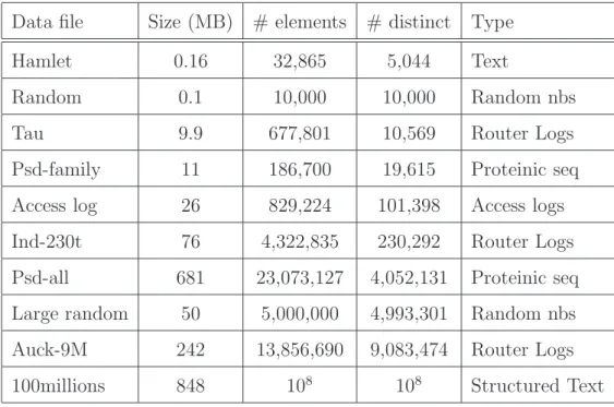
To validate the three families of algorithms we ran simulations using files of different kinds and sizes. Examples of these files are given in Figure 3. The size range is from few tens of thousands to tens of millions. Files are very diverse; english plays, e.g. Hamlet; router logs (traces available on the website of the NLANR Measurement and Network Analysis Group http://moat.nlanr.net);
Data file Size (MB) # elements # distinct Type
Hamlet 0.16 32,865 5,044 Text
Random 0.1 10,000 10,000 Random nbs
Tau 9.9 677,801 10,569 Router Logs
Psd-family 11 186,700 19,615 Proteinic seq
Access log 26 829,224 101,398 Access logs
Ind-230t 76 4,322,835 230,292 Router Logs
Psd-all 681 23,073,127 4,052,131 Proteinic seq
Large random 50 5,000,000 4,993,301 Random nbs
Auck-9M 242 13,856,690 9,083,474 Router Logs
100millions 848 108 108 Structured Text
Fig. 3. Simulation data suite.
access logs collected at the gateway of the INRIA Rocquencourt campus; pro-teinic sequences (available from the website of the database group of the Uni-versity of Washington3); random number files and consecutive number files.
Random is a set of 500 files containing 10,000 integers chosen uniformly at random. In the following section, the results for these files are an average over the set. 100millions is a list of 100 million consecutive integers. This very structured set is used to verify the good alea properties of the algorithm.
5.2 Validation of the algorithms
We estimate here the number of distinct elements of the data suite files of Section 5.1 using estimators of the three families of estimates. Figure 4 shows a summary of typical results for the estimators built with the third minimum. Each of the three horizontal blocks corresponds to results for the estimator of one family. Different columns correspond to simulations with different values of m leading to different expected precisions (recall that m is the number of simulated experiences during the stochastic averaging process). A number in the table is the experimental relative error, i.e. the difference in percents between the estimate given by the algorithm and the exact value. For example, the number of different connections in the trace file Ind-230t is estimated with a precision of respectively 1.4 %, 4.7 % and 4.0 % by the estimates of the Inverse, Square Root and Logarithm Families. The third set of results,
m 4 8 16 32 64 128 256 512 1024 %th 50 35.4 25 17.7 12.5 8.8 6.25 4.4 3.1 1 M(3) Random 53.2 33.5 25.9 17.9 14.3 9.4 6.1 4.3 3.0 Ind − 230t 31.0 32.9 10.4 1.9 10.5 9.4 1.4 0.3 0.05 Auck − 9M 10.3 4.0 5.1 10.0 2.8 3.9 1.7 1.8 3.0 %th 36.3 25.7 18.1 12.8 9.1 6.4 4.5 3.2 2.3 1 √ M(3) Random 38.4 26.5 18.0 13.4 9.0 6.2 4.6 3.1 2.1 Ind − 230t 27.9 18.0 5.9 1.9 10.7 11.4 2.3 0.5 0.15 Auck − 9M 10.6 4.7 2.1 4.7 5.2 0.08 0.3 2.1 2.9 %th 34.0 23.1 16.0 11.2 7.9 5.6 3.9 2.8 2.0 ln 1 M(3) Random 34.9 22.3 16.0 11.8 8.0 5.5 4.0 2.6 1.9 Ind − 230t 25.8 3.5 1.3 4.9 10.6 12.2 3.2 1.2 0.3 Auck − 9M 10.7 6.1 0.2 0.6 6.2 2.7 0.6 2.7 2.9
Fig. 4. Relative error (in percents) of the estimates of the three families.
Random, corresponding to mean results over simulations on 500 files, validates the precision given in Theorem 1. We point out that the numbers are close to what is predicted by the theory. For example for m = 32, we obtain precisions of 17.9, 13.1 and 11.8 for the three families to compare with the expected precisions 17.7, 12.8 and 11.2, indicated in the lines %th in Figure 4. It validates the algorithms: the asymptotic regime is quickly reached and the values are well distributed by the hashing function.
The algorithms have a very good tradeoff between the precision and the size of the memory. For instance, for m = 1024, the algorithm of the Logarithm Family built on the third minimum (the best practical estimate) stores the three first minimums for m buckets. Using 32-bit floating numbers, this cor-responds to a memory of only 12KB. This is sufficient to build an estimate with accuracy of order 2 percents for a multiset with several million elements.
5.3 Execution time
The algorithms are motivated by the processing of very large multisets of data, in particular in the field of inline analysis of internet traffic. Most backbone networks operated today are Synchronous Optical NETworks (SONET). In these networks, the links are optical fibers classified according to their
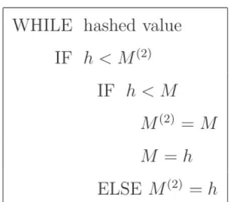
ca-WHILE hashed value IF h < M(2) IF h < M M(2) = M M = h ELSE M(2) = h Fig. 5. Internal loop for k = 2.
Test files Mc Rate Rate Mc/ Mc/ wc -w/ sort -u | wc/ (s) (MB/s) (Me/s) cat -T wc -l Mc Mc Tau 0.20 50. 3.4 4.0 10. 1.4 75.0 psd-family 0.17 65. 3.4 4.0 10. 1.4 58.8 access log 0.43 60. 1.9 3.3 11. 1.7 81.4 psd-all 11.7 58. 2.0 3.0 9.2 1.6 70.2 large random 1.1 45. 4.5 3.5 7.9 1.2 50.5 Auck-9M 4.6 53. 3.0 3.2 8.6 1.5 65.9 100millions 21.7 39.1 4.6 3.6 6.7 1.35 31.5 Fig. 6. Mincount (Mc) execution times on the files of the data suite, correspond-ing throughput (in millions of bytes per second (MB/s) and millions of elements per second (Me/s)) and timing ratios between Mincount and common Unix com-mands.
pacity from OC-1 (51.84 Mbps) to widely used OC-192 (10 Gbps) and even OC-768 (40 Gbps). It is crucial for carriers to know characteristics of the traffic for network monitoring and network design, see [11] and [18]. In particular, Estan, Varghese and Fisk inventory four major uses of the number of distinct connection statistics in [7]: general monitoring, detection of port scan attacks, detection of denial of service attacks (DoS attacks), and study of the spread-ing of a worm. At 40 Gbps speed a new packet arrives every 60 nanoseconds, assuming an average packet size of 300 bytes, see [11]. This allows only 150 operations per packet on a 2.5 GHz processor ignoring the significant time taken by the data to enter the processor. Thus execution times of algorithms are crucial in this context. The algorithms of the three families are mainly composed of a very simple internal loop that finds the k-th minimum of a multiset. This loop is given for k = 2 in Figure 5. Typically, only one com-parison is performed in each loop iteration. Hence the algorithms are quite efficient.
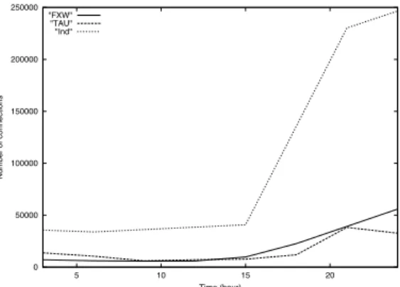
0 50000 100000 150000 200000 250000 5 10 15 20 Number of connections Time (hour) "FXW" "TAU" "Ind"
Fig. 7. Connections Peak during the Spreading of the Code Red Worm
Mincount, an optimized implementation of the best practical estimate, is used here. Figure 6 shows Mincount execution times in seconds while pro-cessing the files of the data suite. The algorithm takes only few seconds to give an estimate of the cardinality of files with millions of elements. For example, 4.8 seconds are enough to process the trace Auck-9M with 13 million elements, including 9 million distinct ones. This corresponds to a rate of 53 MegaBytes per second or 3 million elements per second. The following Unix command are used as references for the execution time: cat -T that reads the file and displays tab characters as ˆI; wc -l that displays the number of lines of the file; wc -w that displays the number of words of the file; sort -u | wc that gives the number of distinct lines of the file. Figure 6 shows the ratios between the execution time of Mincount and the one of the Unix commands. The algorithm is only between 3 to 4 times slower than the cat -T command that only replace the tab characters in its input by ˆI.
5.4 Code Red attacks
We also simulate an analysis of internet traffic to show a typical use of the algorithms, using Mincount. The NLANR Measurement and Network Anal-ysis Group is doing daily network monitoring. We analyze their traces of July 19th 2001 when a Code Red Worm variant started spreading. The Code Red Worm was designed to spread very fast. More than 359,000 computers were infected in less than 14 hours and at the peak of the infection, more than 2,000 new hosts were infected each minute. We considered three sets of traces: one monitored in the Indiana University MegaPOP (Ind), one in the FIX West facility at NASA Ames (FXW) and the last one in Tel Aviv University (TAU). The traces correspond to a window of 1 minute 30 every three hours. We use the algorithm to estimate within 4 % (m=256) the number of active connec-tions using this link during each of these period of times. Results are shown in Figure 7. It is of course a very rough analysis and more data for other links, other days for example would be needed to give precise conclusions about the spread of the worm. But we are able to detect a change of the activity of
the network caused by the infected hosts in the network. We see a very net increase of the number of active connections starting from 3 pm. For the Ind link, the usual load seems to be around 35,000 connections, 33842 at 6 am. At its peak at midnight we estimate a number of 246,558 connections, around 7 times more. Same observation for TAU and FXW: respectively 7,629 and 9,793 connections at 3 pm and 32,670 and 55,877 at midnight. So, by monitoring a link using our algorithm, we are able to see, using constant memory, unusual increase of the traffic, to detect an attack and to give rough indications about its propagation and extent in some parts of the network.
Acknowledgements. I would like to thank my PhD advisor, Philippe Fla-jolet, for introducing me to the subject of the paper, his help and numerous remarks on this work.
References
[1] Z. Bar-Yossef, T. S. Jayram, R. Kumar, D. Sivakumar, and Luca Tre-visan. Counting distinct elements in a data stream. In RANDOM ’02: Proceedings of the 6th International Workshop on Randomization and Approximation Techniques, pages 1–10. Springer-Verlag, 2002.
[2] A. Broder. On the resemblance and containment of documents. In SE-QUENCES ’97: Proceedings of the Compression and Complexity of Se-quences 1997, page 21, Washington, DC, USA, 1997. IEEE Computer Society.
[3] Andrei Z. Broder. Identifying and filtering near-duplicate documents. In COM ’00: Proceedings of the 11th Annual Symposium on Combinatorial Pattern Matching, pages 1–10, London, UK, 2000. Springer-Verlag. [4] P. Chassaing and L. Gerin. Efficient estimation of the cardinality of
large data sets. In math.ST/0701347, 2007. Extended abstract in the proceedings of the 4th Colloquium on Mathematics and Computer Science, 2006, pages 419-422, 2007.
[5] J. Considine, F. Li, G. Kollios, and J. Byers. Approximate aggregation techniques for sensor databases. In ICDE ’04: Proceedings of the 20th International Conference on Data Engineering, page 449, Washington, DC, USA, 2004. IEEE Computer Society.
[6] M. Durand and P. Flajolet. Loglog counting of large cardinalities. In G. Di Battista and U. Zwick, editors, Annual European Symposium on Algorithms (ESA03), volume 2832 of Lecture Notes in Computer Science, pages 605–617, September 2003.
[7] C. Estan, G. Varghese, and M. Fisk. Bitmap algorithms for counting active flows on high-speed links. IEEE/ACM Trans. Netw., 14(5):925– 937, 2006.
Encyclopae-dia of Mathematics, volume Supplement I, page 28. Kluwer Academic Publishers, Dordrecht, 1997.
[9] P. Flajolet, E. Fusy, O. Gandouet, and F. Meunier. Hyperloglog: the analysis of a near-optimal cardinality estimation algorithm. In Philippe Jacquet, editor, Analysis of Algorithms 2007 (AofA07), Discrete Mathe-matics and Theoretical Computer Science Proceedings, 2007. In press. [10] P. Flajolet and P. N. Martin. Probabilistic counting. In Proceedings of
the 24th Annual Symposium on Foundations of Computer Science, pages 76–82. IEEE Computer Society Press, 1983.
[11] C. Fraleigh, C. Diot, B. Lyles, S. Moon, P. Owezarski, K. Papagiannaki, and F. Tobagi. Design and Deployment of a Passive Monitoring Infras-tructure. In Passive and Active Measurement Workshop, Amsterdam, April 2001.
[12] ´E. Fusy and F. Giroire. Estimating the number of active flows in a data stream over a sliding window. In David Appelgate, editor, Proceedings of the Ninth Workshop on Algorithm Engineering and Experiments and the Fourth Workshop on Analytic Algorithmics and Combinatorics, pages 223–231. SIAM Press, 2007. Proceedings of the New Orleans Conference. [13] L. Getoor, B. Taskar, and D. Koller. Selectivity estimation using
proba-bilistic models. In SIGMOD Conference, 2001.
[14] P. B. Gibbons. Distinct sampling for highly-accurate answers to distinct values queries and event reports. In The VLDB Journal, pages 541–550, 2001.
[15] F. Giroire. Order statistics and estimating cardinalities of massive data sets. In Conrado Martnez, editor, 2005 International Conference on Anal-ysis of Algorithms, volume AD of DMTCS Proceedings, pages 157–166. Discrete Mathematics and Theoretical Computer Science, 2005.
[16] F. Giroire. Directions to use probabilistic algorithms for cardinal-ity for DNA analysis. In Journ´ees Ouvertes Biologie Informatique Math´ematiques (JOBIM 2006), pages 3–5, July 2006.
[17] F. Giroire. R´eseaux, algorithmique et analyse combinatoire de grands ensembles. PhD thesis, Universit´e Paris VI, November 2006.
[18] G. Iannaccone, C. Diot, I. Graham, and N. McKeown. Monitoring very high speed links. In ACM SIGCOMM Internet Measurement Workshop, San Francisco, CA, November 2001.
[19] D. E. Knuth. The Art of Computer Programming, volume 3: Sorting and Searching. Addison-Wesley, 1973.
[20] K.-Y. Whang, B. T. V. Zanden, and H. M. Taylor. A linear-time prob-abilistic counting algorithm for database applications. In TODS 15, 2, pages 208–229, 1990.