Extensive form correlated equilibrium: definition and computational complexity

Extensive Form Correlated Equilibrium:

Definition and Computational Complexity

Bernhard von Stengel

Department of Mathematics, London School of Economics, Houghton St, London WC2A 2AE, United Kingdom

email: stengel@maths.lse.ac.uk

Franc¸oise Forges

CEREMADE, University of Paris – Dauphine,

Place du Marechal de Lattre de Tassigny, 75775 Paris cedex 16, France email: Francoise.Forges@dauphine.fr

March 18, 2006

Abstract: This paper defines the extensive form correlated equilibrium (EFCE) for ex-tensive games with perfect recall. The EFCE concept extends Aumann’s strategic-form correlated equilibrium. Before the game starts, a correlation device generates a move for each information set. This move is recommended to the player only at the time of reaching the information set. The condition of perfect recall in two-player extensive games without chance moves leads to strong restrictions on the players’ information sets, which are of some interest on their own. These are used to characterize the set of EFCE by means of a polynomial number of consistency and incentive constraints for correlating sequences of moves. In contrast, strategic-form correlated equilibria for two-player games without chance moves give rise to NP-hard optimization problems. Similarly, maximizing the pay-off of an EFCE, or of a strategic-form correlated equilibrium, is NP-hard for two-player games with chance moves.

Keywords: Correlated equilibrium, extensive game, polynomial-time computable. JEL classification: C72, C63.

Contents

1 Introduction 3

2 The EFCE concept 5

2.1 Definition of EFCE . . . 6

2.2 Reduced strategies suffice . . . 7

2.3 Example: A signaling game . . . 8

2.4 Relationship to other solution concepts . . . 9

2.5 Discussion and open problems . . . 11

3 Computational complexity 12 3.1 Review of the sequence form . . . 13

3.2 Correlation plans and marginal probabilities . . . 14

3.3 Example of generating move recommendations . . . 16

3.4 Information structure of two-player games without chance moves . . . 18

3.5 Using the consistency constraints . . . 21

3.6 Incentive constraints . . . 25

3.7 Hardness results . . . 27

Acknowledgments 30

1

Introduction

Aumann (1974) defined the concept of correlated equilibrium for games in strategic form. Before the game starts, a device selects private signals from a joint probability distribution and sends them to the players. In the “canonical” interpretation, these signals are strategies that players are recommended to play.

The strategic-form correlated equilibrium can be applied to a game in extensive form. This approach is analogous to expressing a Nash equilibrium as a profile of mixed strate-gies, which are randomizations on the sets of pure strategies. We assume each player has perfect recall. Then, by Kuhn’s theorem (1953), a mixed strategy can be replaced by a be-havior strategy, which defines a randomization over the moves at each information set of the player. A behavior strategy is much less complex than a mixed strategy because it can be specified by a probability for every move, whereas a mixed strategy requires typically an exponential number of probabilities, one for each pure strategy.

This paper proposes a new concept of correlated equilibrium for extensive games, called extensive form correlated equilibrium or EFCE. In the same way as in a Nash equilibrium mixed strategies are replaced by behavior strategies, in an EFCE recommen-dations of pure strategies are replaced by recommenrecommen-dations of moves at information sets. Like in a strategic-form correlated equilibrium, the recommendations to the players are generated before the game starts. However, the recommended move is not revealed to the player before the respective information set is reached. As recommendations become local in this way, players know less. Consequently, the set of EFCE outcomes is larger than the set of strategic-form correlated equilibrium outcomes.

The EFCE is a natural definition of correlated equilibrium for extensive games with perfect recall. It applies to any extensive game with information sets as defined by Kuhn (1953), including games without a well-defined time when each player moves. Earlier extensions of Aumann’s concept applied only to multi-stage games (including Bayesian games and stochastic games) that have a special time and information structure. These known approaches are discussed in Section 2.4 below.

For games in strategic form, correlated equilibria are easier to compute than Nash equilibria. The incentive constraints that define the set of correlated equilibria of a game are linear inequalities in terms of the joint probabilities over strategy profiles. An incen-tive constraint compares any two strategies of a player, so the number of these constraints is polynomial in the size of the strategic form. Consequently, finding a correlated equi-librium with, say, maximum payoff sum amounts to solving a linear program, so this can done in polynomial time. In contrast, finding a Nash equilibrium with maximum payoff sum defines an NP-hard optimization problem (Gilboa and Zemel (1989), Conitzer and Sandholm (2003); see Garey and Johnson (1979) or Papadimitriou (1994) for notions of computational complexity).

Linear programming can also be applied to computing Nash equilibria when the strate-gic-form game has two players and zero-sum payoffs. When the game is given in extensive form, its strategic form has an exponentially larger amount of data than the game tree, so

the game cannot be solved in polynomial time using the strategic form. The strategic form is therefore computationally intractable for larger extensive games.

However, extensive two-player zero-sum games with perfect recall can still be solved in polynomial time in the tree size, as shown by Romanovskii (1962), Koller and Megiddo (1992), and von Stengel (1996). These methods use the sequence form of an extensive game which represents a behavior strategy by its realization probabilities for sequences of moves along a path in the game tree. These realization probabilities can be characterized by linear equations, one for each information set. Thereby, the sequence form provides a strategic description that has the same size as the game tree, unlike the exponentially large strategic form.

Given an extensive game with perfect recall, is there a “sequence form” to compute a strategic-form correlated equilibrium with, say, maximum payoff sum in polynomial time? The answer is negative because this problem is NP-hard (Chu and Halpern (2001); see also Theorem 3.10 below). The set of correlated equilibria can therefore not be characterized by a polynomial number of inequalities in the size of the game tree, assuming that P 6= NP. Chu and Halpern’s construction applies to extensive games of two players with an initial chance move. In Theorem 3.11, we show that even for an extensive two-player game without chance moves, a strategic-form correlated equilibrium with maximum payoff sum is hard to compute.

In contrast, extensive form correlated equilibria are computationally tractable for two-player games without chance moves. We show that a polynomial number of linear con-straints suffice to characterize EFCE for these games. These concon-straints extend the se-quence form constraints as used for Nash equilibria. They define joint probabilities for correlating moves at any two information sets of the two players by means of suitable con-sistency and incentive conditions. From these probabilities, the recommended moves are generated for one information set at a time, taking earlier recommendations into account. This specifies the correlation device compactly, without explicitly using probabilities for strategy profiles.

The polynomial-time computability of EFCE for two-player games without chance moves is not straightforward. The consistency constraints on the marginal probabilities of moves that are correlated across information sets are in general only necessary condi-tions. In extensive games with two players and without chance moves, these constraints are also sufficient to describe the set of EFCE. For such games, the condition of perfect recall imposes strong restrictions on the players’ information sets (see Section 3.4), for example a unique partial “time order” among them. These properties may be of some interest by themselves. The most important consequence is that the generation of a rec-ommended move at a player’s information set can be based on a unique earlier sequence of moves by the other player (see Lemma 3.3(c) and (9) in the proof of Theorem 3.8). Because the number of sequences, as opposed to strategies, is polynomial, this reduces the computational complexity.

The EFCE concept can be regarded as the correlated analog of a Nash equilibrium in behavior strategies. It is closer in spirit to the dynamic description of the game by a tree than the strategic-form correlated equilibrium. At the same time, the correlation

de-vice does not have additional power in the sense of observing the game state, because it generates signals at the beginning of the game. In addition, the EFCE concept is compu-tationally tractable, at least for two-player games without chance moves. The EFCE also seems to be the first case of a game-theoretic concept where the introduction of chance moves marks the transition from polynomial-time solvable to NP-hard problems.

Interestingly, Papadimitriou (2005) describes how to find a correlated equilibrium for a compactly represented multi-player game in polynomial time even though finding a correlated equilibrium with maximum payoff sum is NP-hard. That is, maximizing the payoff sum is a stronger computational requirement than merely finding one correlated equilibrium. The compactly represented games considered by Papadimitriou encompass a wide class of games, but not games in extensive form. It is open whether his approach can be applied to the EFCE concept for extensive games with chance moves or with more than two players.

The two main parts of this paper treat the conceptual and the computational aspects of EFCE. In the first part, we first define the EFCE concept. Then we observe that the EFCE can be defined in “canonical form” and by generating only reduced strategy profiles. A signaling game shows that an EFCE can be “type-revealing” when this is not possible with a Nash or strategic-form correlated equilibrium. We then compare the EFCE concepts with related other notions of correlated equilibria. In conclusion, we mention open conceptual problems. Most of our mathematical observations are straightforward, so that we do not state them as theorems with proofs.

The second part of this paper is concerned with computational complexity, and much more technical. Our positive result, a compact description of the set of EFCE, holds for two-player extensive games with perfect recall and without chance moves. We have to prove carefully how the “consistency constraints” describe probabilities for generating moves, because the games we consider have no clear “stages” (see, for example, Figure 6). On the other hand, the consistency constraints provide sufficient structure for generating move recommendations in an unambiguous way. The computational difficulties of more general games with chance moves, and of strategic-form correlated equilibria, are consid-ered at the end of this paper.

2

The EFCE concept

The EFCE concept is defined in Section 2.1. As shown in Section 2.2, an EFCE can be defined with a correlation device that generates reduced strategy profiles. A game with costless signals illustrates the use of EFCE, as explained in Section 2.3. In Section 2.4, we compare the EFCE with other concepts of correlated equilibria that have been defined for games with special time or information structures. Open problems that arise from a conceptual viewpoint are discussed in Section 2.5.

2.1

Definition of EFCE

We use the following standard terminology for extensive games. Let N be the finite set of players. The game tree is a finite directed tree, that is, a directed graph with a distinguished node, the root, from which there is a unique path to any other node. The non-terminal decision nodes of the game tree are partitioned into information sets. Each information set belongs to exactly one player i. The set of all information sets of player i is denoted Hi.

The set of choices or moves at an information set h is denoted Ch. Each node in h has |Ch|

outgoing edges, which are labeled with the moves in Ch.

We assume each player has perfect recall, defined as follows. Without loss of gen-erality, choice sets Ch and Ck for h 6= k are considered disjoint. A sequence of moves of

a particular player is a sequence of his moves (ignoring the moves of the other players) along the path from the root to some node in the game tree. By definition, player i has perfect recall if all nodes in an information set h in Hi define the same sequence σh of

moves for player i.

The set of pure strategies of player i is

Σi=

∏

h∈Hi

Ch. (1)

The set of all strategy profiles is

Σ=

∏

i∈N

Σi. (2)

Definition 2.1. A (canonical) correlation device is a probability distributionµ onΣ. A correlation device µ makes recommendations to the players by picking a strategy profileπ according to the distribution µ, and privately recommending the componentπi ofπto each player i for play. It defines a strategic-form correlated equilibrium if no player can gain by unilaterally deviating from the recommended strategy, given his posterior on the recommendations to the other players (see Aumann (1974)). We define an extensive form correlated equilibrium also by means of a correlation device, but with a different way of giving recommendations to the players.

Definition 2.2. Given a correlation deviceµ as in Definition 2.1, consider the extended game in which a chance move first selects a strategy profile π according to µ. Then, whenever a player i reaches an information set h in Hi, he receives the move c at h specified

inπ as a signal, interpreted as a recommendation to play c. An extensive form correlated equilibrium (EFCE) is a Nash equilibrium of such an extended game in which the players follow their recommendations.

In an EFCE, the strategy profile selected according to the device defines a move c for each information set h of each player i, which is revealed to player i only when he reaches h. It is optimal for the player to follow the recommended move, assuming that all future moves, including of the player himself, are followed as recommended. However, when a player considers a deviation from a recommended move, he is not obliged to

follow subsequent recommendations. This distinguishes the EFCE from the agent normal form correlated equilibrium, which is a correlated equilibrium where at every information set, the move is chosen by a different agent (see also Section 2.4).

The above description of extensive form correlated equilibria is in “canonical form”. That is, the recommendations to players are moves to be made at information sets and not arbitrary signals. In the same way as for strategic-form correlated equilibria, this can be assumed without loss of generality (see Forges (1986a)).

2.2

Reduced strategies suffice

In the reduced strategic form of an extensive game, strategies of a player that differ in moves at information sets which are unreachable due to an own earlier move are iden-tified.1 A reduced strategy can still be considered as a tuple of moves, except that the unspecified move at any unreachable information set is denoted by a new symbol, for example a star “∗”, which does not belong to any set of moves Ch.

We denote the set of all reduced strategies of player i byΣ∗_i, and the set of all reduced strategy profiles by

Σ∗₌

∏

i∈N Σ∗

i. (3)

By construction, the payoffs for a profile of reduced strategies are uniquely given as in the strategic form. This defines the reduced strategic form of the extensive game.

In Definition 2.1, a correlation device is defined on Σ, that is, using the unreduced strategic form. We now re-define a correlation device to be a probability distribution on Σ∗. Any correlated equilibrium that is specified using the unreduced strategic form can be considered as a correlated equilibrium for the reduced strategic form. This is achieved by defining the probability for a profile π∗ of reduced strategies as the sum of the probabilities of the unreduced strategy profilesπ that agree withπ∗(in the sense that wheneverπ∗ specifies a move other than “∗” at an information set, thenπ specifies the same move). Because the incentive constraints hold for the unreduced strategies, and payoffs are identical, appropriate sums of these give rise to the incentive constraints for the reduced strategies, which therefore hold as well.

Conversely, any correlated equilibrium for the reduced strategic form can be applied to the unreduced strategic form by arbitrarily defining a move for every unreachable in-formation set (which is “∗”, that is, undefined, in the reduced strategy profile), thereby defining a particular unreduced strategy to be selected by the correlation device.

In the same manner, an EFCE can be defined by assigning probabilities only to re-duced strategy profiles. This defines an EFCE for unrere-duced strategy profiles by recom-mending an arbitrary move at each unreachable information set. Conversely, consider an EFCE defined using unreduced strategy profiles as in Definition 2.2. Then, just as in the strategic form, this gives rise to an EFCE for reduced profiles, as follows. In the strategy

1_{We define the reduced strategic form in this way because it only depends on the game tree structure and}

profileπ generated by the correlation device, any recommendation at an unreachable in-formation set is replaced by “∗”. Suppose a player deviates from his recommended move at some information set, and gets a higher payoff by subsequently using moves at pre-viously unreachable information sets where he only gets the recommendation “∗”. Then the player could profitably deviate in the same way when getting recommendations of moves for these information sets as inπ, which he ignores. This contradicts the assumed equilibrium property.

2.3

Example: A signaling game

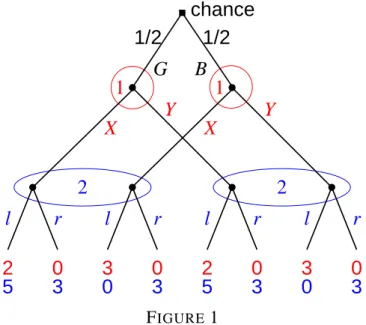
Figure 1 shows an example of an extensive game. This is a signaling game as discussed by Spence (1973), Cho and Kreps (1987), and Gibbons (1992, Section 4.2), but with costless signals. Player 1, a student, can be with equal probability of a good (G) or bad (B) type. He applies for a summer research job with a professor, player 2. Player 1 sends a costless signal X or Y . The professor can distinguish the signals but not the type of player 1, as shown by her two information sets. She can either let the student work with her (l) or refuse to do so (r). Move r always gives the pair of payoffs (0, 3) to players 1 and 2, but l results in (2, 5) for G versus (3, 0) for B.

chance

1/2

1/2

0

3

0

3

5

3

0

2

0

3

0

3

5

3

0

2

l

r

l

r

l

r

l

r

Y

X

Y

X

G

1

1

2

B

2

In any Nash equilibrium of this game, player 2 refuses to work with the student, choos-ing r at both information sets. Otherwise, any positive probability for l would induce both types of player 1 to send a (not necessarily unique) signal where that probability of accep-tance is the highest; hence, for at least one signal, l is not optimal for player 2 because the bad type is at least as likely as the good type. With player 2 always playing r, the signal sent by player 1 does not matter (he gets payoff 0 anyhow), as long as in no information set of player 2, the conditional probability for G versus B is so high as to make her switch to l.

Similarly, in every strategic-form correlated equilibrium, player 2 is never recom-mended to choose move l, because otherwise the bad type would “imitate” the good type by sending the signal where player 2 would choose l. So in this game, the sets of Nash and correlated equilibrium outcomes coincide.

However, there is an EFCE with better payoff to both players compared to the outcome with payoff pair (0, 3): A signal X or Y is chosen with equal probability for type G, and player 2 is told to accept (move l) when receiving the chosen signal and to refuse (move r) when receiving the other signal. The bad type B is given an arbitrary recommendation which is independent of the recommendation to type G. Because the move recommended to G is unknown to B, the bad type cannot distinguish the two signals and, no matter what he does, will match the signal of G with probability 1/2. When player 2 receives the signal chosen for G, it is therefore twice as likely to come from G rather than from B, so that her expected payoff 10/3 for choosing l is higher than 3 when she chose r. When she receives the wrong signal, it comes from B with certainty, and then the best reply is certainly r with payoff 3. The expected payoffs to the two players in this EFCE are 1.75 to player 1 and 3.25 to player 2. In a more elaborate game with M signals instead of just two signals, where the bad type can only guess the correct signal with probability 1/M, the pair of expected payoffs is (1 + 1.5/M, 4 − 1.5/M).

In the terminology of signaling games, any Nash or correlated equilibrium is the de-scribed “pooling equilibrium” with payoff pair (0, 3). This is due to the fact that signals are costless and therefore uninformative. In contrast, the EFCE concept allows for a “par-tially revealing” equilibrium, where signals can distinguish the types, which has better payoffs for both players.

2.4

Relationship to other solution concepts

Our definition of an EFCE generalizes the Nash equilibrium in behavior strategies and applies to any game in extensive form (with perfect recall). Other extensions of Aumann’s strategic-form correlated equilibrium have been proposed in order to take account of the dynamic structure of specific classes of games, namely Bayesian games and multi-stage games.

In a Bayesian game, every player has a type which can be represented by an informa-tion set. Players move only once and simultaneously. For Bayesian games, the agent nor-mal form correlated equilibrium studied in, e.g., Forges (1986b), Samuelson and Zhang (1989), Cotter (1991), and Forges (1993), exactly coincides with the EFCE.

However, in general extensive form games, the set of agent normal form correlated equilibrium outcomes can be larger than the set of EFCE outcomes. An easy example is a one-player game where the player moves twice, first choosing either “Out” and receiving zero, or “In” and then choosing again between “Out” with payoff zero or “In” with payoff one. If the two agents at the two decision points both choose “Out”, this defines an agent normal form correlated equilibrium, but not an EFCE.

In multi-stage games, the best known extension of the strategic-form correlated equi-librium is the communication equiequi-librium introduced by Myerson (1986) and Forges

(1986a). The underlying canonical scenario is that at every stage of the game, every player is invited to report his new information to a communication device (with perfect memory), which in turn makes private recommendations to the players. In a canonical equilibrium, players are truthful and obedient at every stage. This solution concept differs from the EFCE in two respects: First, the players can send inputs to the device. Second, the outputs can depend on the players’ inputs but not on their true information, which is unknown to the device. The device is only informed about the stage (and remembers what players have told it) but cannot distinguish between different information sets of a player at the same stage when generating its outputs. In contrast, the recommendations given in an EFCE are local even at the same stage, as the example in Figure 1 shows. In that example, any communication equilibrium gives only the payoff pair (0, 3). That is, the set of communication equilibrium outcomes in that example is strictly included in the set of EFCE outcomes. The reverse inclusion can also hold. For example, consider a game (described by Forges (1986a), p. 1383) where player 1 learns a move of nature but has only one move himself (like only one signal, say X , in Figure 1). Player 2 does not know the move of nature but would profit from doing so, along with player 1 who has the same payoffs. In a communication equilibrium, player 1 could inform player 2 to their joint benefit, but not in an EFCE.

Like the communication equilibrium, the autonomous correlated equilibrium (Forges (1986a)) applies to multistage games; the players receive outputs at every stage, but can-not make any inputs to the device. In the canonical version of the solution concept, the output to every player at every stage is a mapping telling him which move to choose at that stage as a function of his information (i.e., the relevant part of his strategy for the given stage). However, unlike in an EFCE, the respective signal is known to the player for the entire stage and not only locally for each information set.2 Obviously, every strategic-form correlated equilibrium outcome is an autonomous correlated equilibrium outcome, but the converse is not true in general, like in a battle of sexes game preceded by a suitable outside option (see Myerson (1986, Fig. 2)). Similarly, the set of autonomous correlated equilib-rium outcomes is included in the set of EFCE outcomes, and the inclusion may be strict, as shown in the example of the previous section. The same holds in the class of games we consider later, namely two-player games without chance moves (see Section 3.3).

Solan (2001) defines a concept of communication equilibrium for stochastic games where the device knows the game state and all past moves, which are also known to all players. He proves that this concept is outcome equivalent to the autonomous correlated equilibrium. Therefore, in stochastic games, or other games where the players have sym-metric information, the equilibrium outcomes for these concepts and the EFCE coincide.

Kamien, Tauman, and Zamir (1990) and Zamir, Kamien, and Tauman (1990) study extensive games with a single initial chance move. The game is modified by introducing a disinterested additional player (the “maven”) who can reveal any partial information about the chance move to each player. In some games, the resulting set of payoffs has

2_{In Forges (1986a, p. 1378), a correlated equilibrium based on an autonomous device is called “extensive}

form correlated equilibrium”, but this is now typically referred to as “autonomous correlated equilibrium”. We suggest now to use “EFCE” in our sense.

some similarity with that obtainable in an EFCE. However, the correlation device used in an EFCE is weaker than such a maven, for the following reasons: Recommendations are generated at the beginning of the game. The device does not observe play, and “knows” the game state only implicitly under the assumption that players observe their recommended moves. The device cannot make recommendations conditional on game states that have been determined by a chance move.

Moulin and Vial (1978) proposed a “simple extension” of Aumann’s (1974) correlated equilibrium that is completely different from the ones reviewed above. Like the strategic-form correlated equilibrium, their solution concept, which is sometimes referred to as coarse correlated equilibrium (Young (2004)), is described by a probability distribution

µ on pure strategy profiles and applies to the strategic form of the game. However, the players do not receive any recommendation on how to play the game: each of them can just choose to either adhere toµ and get the corresponding correlated expected payoff or to deviate ex ante, by picking some strategy. The coarse correlated equilibrium conditions express that no player can gain by unilaterally deviating ex ante. Moulin and Vial’s so-lution concept assumes in effect some limited commitment from the players, who let the correlation device play for them at equilibrium.

Every EFCE defines a coarse correlated equilibrium: Namely, given an EFCE, it is clear that no player can benefit by ignoring the recommendations of the device at his information sets and deviating unilaterally before the beginning of the extensive form game.

2.5

Discussion and open problems

As observed in the comparison with other solution concepts, the EFCE can give rise to a larger set of outcomes than a communication equilibrium. A device which can give every player a recommendation that depends on a player’s information set, which in a Bayesian game represents the player’s type, may be considered rather powerful. That is, the ex-tended game that defines the EFCE as in Definition 2.2 can be viewed as changing the game quite substantially. However, we think this is a natural approach when information sets define the rules of the game, rather than defining types which may be not easily “ver-ifiable”. In other words, our concept applies to games with imperfect information rather than games with incomplete information. The standard equivalence between these games (Harsanyi (1967)), which is undisputed for Nash equilibria, may become controversial for correlated equilibria.

In distinction to communication equilibria where players can send signals to the de-vice, an EFCE does not change the game by giving additional moves to the players. The recommended move is associated with the information set of the player, but this does not assume an omniscient device that knows the game state.

An interpretation of the moves that are generated in an EFCE would be recommen-dations that are put into “sealed envelopes” which a player can only open when reaching the respective information set. We assume that the players cannot obtain the information earlier, in the same way as we assume that the information sets describe the rules of the

game which the players must obey. An interesting open question is how to implement “sealed envelopes” in this context by cryptographic techniques. A starting point may be Dodis, Halevi, and Rabin (2000) and Urbano and Vila (2002) who use cryptography to replace the mediator in a correlated equilibrium.

Does the EFCE concept reflect “common knowledge of rationality for extensive games with Bayesian players”, in analogy to Aumann’s (1987) interpretation for strategic-form games? This should be confined to a static description of the game. In a dynamic de-scription, rationality would also mean sequential rationality. Such a concept would lead to refinements such as subgame perfect, or sequential equilibrium. This is not the case for EFCE which include all Nash equilibria, including those that are not sequential. The EFCE concept seems well suited to address refinements such as perfection; see Dhillon and Mertens (1996) or Gerardi (2004, p. 117).

In Forges (1993), Aumann’s (1987) approach is extended to Bayesian games. The corresponding concept of a “belief-invariant Bayesian solution” is described by a prob-ability distribution over types and actions such that the marginal distribution on types is that of the original game. In addition, the action of one player, given his own type, is con-ditionally independent of the other players’ types. The incentive constraints express that a player should choose the action recommended by an omniscient mediator who uses this distribution. Clearly, any agent normal form correlated equilibrium (which coincides with the EFCE in a Bayesian game), induces a belief-invariant Bayesian solution. However, contrary to the claim in Forges (1993, Proposition 3), there may be other belief-invariant Bayesian solutions; see Forges (2006).

3

Computational complexity

So far, we have argued that the EFCE is a “natural” concept for games in extensive form. In this second part of the paper, we show that the EFCE is also attractive from a computa-tional point of view. We will show that the set of EFCE has a compact description given by a polynomial number of inequalities in the size of the game tree, provided the game has only two players and no chance moves. The last Section 3.7 gives hardness results showing that, given an extensive game, such a compact description cannot be expected for the set of strategic-form correlated equilibria, and also not for the set of EFCE if the game has chance moves (or a third player).

In an EFCE, the device recommends moves rather than strategies to the players. One motivation for this is a potential reduction in computational complexity, because the corre-sponding incentive constraints compare any two moves rather than any two pure strategies of a player. In addition to incentive constraints, we need consistency constraints that ex-press how the moves at any two information sets are correlated.

First, we review in Section 3.1 the sequence form. This is a compact description of “re-alization plans” that specify the probabilities for playing sequences of moves, which can be translated to behavior strategy probabilities. Section 3.2 describes how to extend the constraints for realization plans to constraints for joint probabilities for pairs of sequences

(we always consider only two players), which we call “correlation plans”. Section 3.3 gives an example that illustrates the use of these constraints.

In general, the consistency constraints apply only to mutually “relevant” information sets that share a path in the game tree, as explained in Section 3.4. That section also de-scribes implications of perfect recall for the information sets in games with two players and without chance moves, and defines the concept of a “reference sequence”, which is used to generate move recommendations. Based on these technical preliminaries, Sec-tion 3.5 shows how to use the consistency constraints as a compact descripSec-tion of a corre-lation device as used in an EFCE. The incentive constraints are described in Section 3.6. Computational difficulties that arise in games with chance moves are discussed in the final Section 3.7.

3.1

Review of the sequence form

The sequence form of an extensive game is similar to the reduced strategic form, but uses sequences of moves of a player instead of reduced strategies. Since player i has perfect recall, all nodes in an information set h in Hi define the same sequence σh of moves for

player i (see Section 2.1). The sequenceσh leading to h can be extended by an arbitrary move c in Ch. Hence, any move c at h is the last move of a unique sequenceσhc. This

defines all possible sequences of a player except for the empty sequence /0. The set of sequences of player i is denoted Si, so

Si= { /0 } ∪ {σhc | h ∈ Hi, c ∈ Ch}.

We will use the sequence form for characterizing EFCE of two-player games (without chance moves). Then we denote sequences of player 1 byσ and sequences of player 2 byτ, and for readability the sequence leading to an information set k of player 2 byτk.

The sequence form is applied to Nash equilibria as follows (see also von Stengel (1996), Koller, Megiddo, and von Stengel (1996), or von Stengel, van den Elzen, and Talman (2002)). Sequences are played randomly according to realization plans. A real-ization plan x for player 1 is given by nonnegative real numbers x(σ) forσ ∈ S1, and a

realization plan y for player 2 by nonnegative numbers y(τ) forτ ∈ S2. They denote the

realization probabilities for the sequencesσ andτ when the players use mixed strategies. Realization plans are characterized by the equations

x( /0) = 1,

∑

∑

The reason is that equations (4) hold when a player uses a behavior strategy, in particular a pure strategy, and hence also for a mixed strategy which is a convex combination of pure strategies. A realization plan x (and analogously, y) fulfilling (4) results from a behavior strategy of player 1 (respectively, player 2) that chooses move c at an information set

h ∈ H1with probability x(σhc)/x(σh) if x(σh) > 0 and arbitrarily if x(σh) = 0. This yields

a canonical proof of the theorem of Kuhn (1953) that asserts that a player with perfect recall can replace any mixed strategy by an equivalent behavior strategy. The behavior at h is unspecified if x(σh) = 0, which means that h is unreachable due to an earlier own move. Not specifying the behavior at such information sets is exactly what is done in the reduced strategic form.

Sequence form payoffs are defined for profiles of sequences whenever these lead to a leaf (terminal node) of the game tree, multiplied by the probabilities of chance moves on the path to the leaf. Here, we consider the special case of two players and no chance moves, and extend the sequence form to a compact description of the set of EFCE.

The sequence form is much smaller than the reduced strategic form, because a real-ization plan is described by probabilities for the sequences of the player, whose number is the number of his moves. In contrast, a mixed strategy is described by probabilities for all pure strategies of the player, whose number is generally exponential in the size of the game tree.3 A polynomial number of constraints, namely one equation (4) for each information set (and nonnegativity), characterizes realization plans. These constraints can be used to describe Nash equilibria, as explained in the papers on the sequence form cited above.

3.2

Correlation plans and marginal probabilities

In the following sections, we consider an extensive two-player game with perfect recall and without chance moves. Then any leaf of the game tree defines a unique pair (σ,τ) of sequences of the two players. Let a(σ,τ) and b(σ,τ) denote the respective payoffs to the players at that leaf. Then if the two players use the realization plans x and y, their expected payoffs are given by the expressions, bilinear in x and y,

∑

σ,τx(σ) y(τ) a(σ,τ) , σ

∑

respectively. The expressions in (5) represent the sums over all leaves of the payoffs multiplied by the probabilities of reaching the leaves. The sums in (5) may be taken over allσ ∈ S1andτ ∈ S2by assuming that a(σ,τ) = b(σ,τ) = 0 whenever the sequence pair

(σ,τ) does not lead to a leaf. This is useful when using matrix notation, where the payoffs in the sequence form are entries a(σ,τ) and b(σ,τ) of sparse |S1| × |S2| payoff matrices

and x and y are regarded as vectors.

In order to describe an EFCE, the product x(σ) y(τ) in (5) of the realization probabili-ties forσ in S1andτ in S2will be replaced by a more general joint realization probability

z(σ,τ) that the pair of sequences (σ,τ) is recommended to the two players, for a suit-able correlation deviceµ, as far as this probability is relevant. These probabilities z(σ,τ) define what we call a correlation plan for the game.

3_{A class of games with exponentially large reduced strategic form is described by von Stengel, van den}

As a tentative definition, given in full in Definition 3.7 below, a correlation plan is a function z : S1× S2 → R for which there is a probability distribution µ on the set of

reduced strategy profilesΣ∗such that for each sequence pair (σ,τ),

z(σ,τ) =

∑

(p1,p2) ∈Σ∗ (p1,p2) agrees with (σ,τ)

µ(p1, p2). (6)

Here, the reduced pure strategy pair (p1, p2) agrees with (σ,τ) if p1chooses all the moves

inσ and p2chooses all the moves inτ.

In an EFCE, a player gets a move recommendation when reaching an information set. The move corresponds uniquely to a sequence ending in that move. For player 1, say, the sequence denotes a row of the |S1| × |S2| correlation plan matrix. From this row, player 1

should have a posterior distribution on the recommendations to player 2. This behavior of player 2 must be specified not only when player 1 follows a recommendation, but also when player 1 deviates, so that player 1 can decide if the own recommendation is optimal; see also the example in Section 3.3. The recommendations to player 2 off the equilibrium path are therefore important, so the collection of recommended moves to player 2 has to define a reduced strategy. Otherwise, one could simply choose a distribution on the leaves of the tree (with a correlation plan that is a sparse matrix like the payoff matrix), and merely recommend to the players the pair of sequences corresponding to the selected leaf. Our first approach is therefore to define a correlation plan z as a full matrix. Except for a scalar factor, a column of this matrix should be a realization plan of player 1, and a row should be a realization plan of player 2. According to (4) (except for the equations x/0= 1

and y/0= 1 that define the scalar factor), this means that for allτ ∈ S2, h ∈ H1,σ ∈ S1, and

k ∈ H2,

∑

∑

z( /0, /0) = 1, z(σ,τ) ≥ 0 (σ ∈ S1,τ ∈ S2). (8)

Clearly, the constraints (7) and (8) hold for the special case z(σ,τ) = x(σ)y(τ) where x and y are realization plans. With properly defined incentive constraints that make it an EFCE, such a correlation plan of rank one should define a Nash equilibrium. In particular, if x and y stand for reduced pure strategies, where each sequenceσ or τ is chosen with probability zero or one, then the probabilities z(σ,τ) = x(σ)y(τ) are also zero or one, and equations (7) and (8) hold. For any convex combination of pure strategy pairs, as in an EFCE, (7) and (8) therefore hold as well, so these are necessary conditions for a correlation plan.

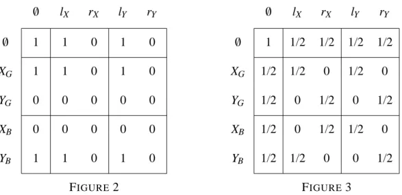
Figure 2 shows a correlation plan defined in this manner for the game in Figure 1. In order to have distinct move names at different information sets, moves X and Y at the information set of the good type are called XGand YG, those of of the bad type XB and YB,

1 1 0 0 1 1 1 0 0 1 0 0 0 0 0 1 1 0 0 1 0 0 0 0 0 /0 XG YG XB YB /0 lX rX lY rY FIGURE 2 /0 XG YG XB YB /0 lX rX lY rY 1 1/2 1/2 1/2 1/2 1/2 1/2 0 0 1/2 1/2 0 1/2 1/2 0 1/2 1/2 0 1/2 0 1/2 0 1/2 0 1/2 FIGURE 3

and the moves of player 2 are lX and rX when she receives signal X and lY and rY when she

receives signal Y . Since both players move only once, every non-empty sequence is just a move. The correlation plan in Figure 2 arises from the pure strategy pair (XGYB, lXlY).

Figure 3 shows a possible assignment of probabilities z(σ,τ) that fulfills (7) and (8). These probabilities are “locally consistent” in the sense that the marginal probability of each move is 1/2. However, they cannot be obtained as a convex combination of pure strategy pairs like the pure strategy pair in Figure 2. Otherwise, one such pair would have to recommend move XGto player 1 and move lX to player 2 to account for the respective

entry 1/2. In that pure strategy pair, given that player 2 is recommended move lX, the

recommendation to player 1 at the other information set must be YB because the move

combination (XB, lX) has probability zero. Similarly, move XG requires that move lY is

recommended to player 2. This pure strategy pair is thus (XGYB, lXlY) as in Figure 2,

but that pair also selects (YB, lY), contradicting Figure 3. This shows that (7) and (8)

do not suffice to characterize the convex hull of pure strategy profiles. For games with chance moves, Theorem 3.10 below shows that this convex set cannot be characterized by a polynomial number of linear inequalities (unless P = NP).

However, we will show that the constraints (7) and (8) suffice to characterize correla-tion plans when the game has only two players and no chance moves.

3.3

Example of generating move recommendations

Figure 4 is a game very similar to Figure 1, except that the initial chance move is replaced by a move by player 1, as if that player “chose his own type”. A similar analysis as in Section 2.3 shows that there is only one outcome in a strategic-form or autonomous correlated equilibrium, or communication equilibrium, which is non-revealing.

Figure 5 gives an example of probabilities z(σ,τ) that fulfill (7) and (8). We demon-strate how to generate a pair of reduced demon-strategies using z, described in general in Sec-tion 3.5 below. We consider only the generaSec-tion of moves, and not any incentive con-straints (treated in Section 3.6), which are in fact violated in Figure 5.

l_Y r_Y l_Y r_Y r_X l_X l_X r_X X_G 0 3 0 3 5 0 3 2 0 3 0 3 5 0 3 2 Y X Y 1 1 2 2 1 G B G B B 1 1/2 1/2 1/4 1/4 1/4 1/4 1/2 1/4 1/4 1/4 0 0 1/4 1/2 1/4 1/4 0 1/4 1/4 0 1/2 1/4 1/4 1/4 0 1/4 0 1/2 1/4 1/4 0 1/4 0 1/4 /0 G B GXG GYG BXB BYB /0 lX rX lY rY FIGURE5 FIGURE 4

The generation of moves starts at the root of the game tree. The information set containing the root belongs to player 1 and has the two moves G and B. We consider a “reference sequence” of the other player, which is here τ = /0 of player 2 because that is the sequence of player 2 leading to the root. This reference sequenceτ determines a column of z describing the probabilities for making a move G or B. In Figure 5, z(G,τ) = z(B,τ) = 1/2. Suppose that move G is chosen. The next information set belongs again to player 1 with moves XG and YG. The reference sequence is stillτ = /0. The moves of

player 1 correspond to the sequences GXGand GYG, which have probabilities z(GXG,τ) =

z(GYG,τ) = 1/4 in Figure 5. These probabilities have to be divided by z(G,τ) to obtain the

conditional probabilities for generating the moves, which are here both 1/2; the respective general equation is (10) below. Suppose that move XGis chosen.

The next information set to be considered (because it still precedes any information set of player 2) is the information set of player 1 with moves XB and YB. However, this

information set is unreachable due to player 1’s earlier move G. Because it suffices to generate only a reduced strategy of player 1 as explained in Section 2.2, no move is rec-ommended at this information set. All information sets of player 1 have been considered, so the generated reduced strategy is (G, XG, ∗); recall that the moves in that strategy are

recommended to player 1 when he reaches his respective information sets.

The remaining information sets belong to player 2. For the information set with moves lX and rX, the reference sequence isσ = GXG because these moves have been generated

for player 1 and reach player 2’s information set. This reference sequenceσ determines a row in Figure 5 where z(σ, lX) = 1/4 and z(σ, rX) = 0. Normalized by dividing by the

probability z(σ, /0) = 1/4 for the incoming sequence /0 of player 2, this means lX is chosen

The information set, say k, of player 2 with moves lY and rY is interesting because it

will not be reached when player 1 plays his recommended moves G and XG. Nevertheless,

a move at k must be recommended to player 2 because player 1 must be able to decide if choosing his recommended move XGis optimal, or if YGis better. Player 1 can only decide

this if he has a posterior over the moves lY or rY of player 2. The reference sequence for

player 2’s selection is againσ = GXG because its last move XGis made at the unique

in-formation set of player 1 that still allows to reach k, described in generality in Section 3.5. According to Figure 5, z(σ, lY) = 1/4 and z(σ, rY) = 0, so lY is also chosen with certainty.

The reduced strategy whose moves are recommended to player 2 is therefore (lX, lY).

The four squares at the bottom right of Figure 5 describe a correlation between the moves at pairs of information sets of player 1 and player 2, with nonzero entries like in Figure 3. However, unlike in Figure 3, these numbers are not only “locally” but also “globally” consistent in the sense that they can arise from a distribution µ on reduced strategy profiles. The reason is that, for example, the moves lY and rY of player 2 are

correlated with either XGand YGor XBand YBof player 1, depending on the first move G

or B of player 1, but not with both move pairs. In contrast, the conflict in Figure 3 arises because G or B is chosen by a chance move.

3.4

Information structure of two-player games without chance moves

In the following sections, we consider only two-player games without chance moves. Using the condition of perfect recall, we describe structural properties of information sets in such games. We then define the concepts of relevant sequence pairs and reference sequences, which we use later in Theorem 3.8.

Definition 3.1. In an extensive game, call any two information sets h and k (possibly of the same player) connected if there is a path from the root to a leaf containing a node of h and a node of k. If the node in h comes earlier on the path, then h is said to precede k.

The following lemma states that two-player games without chance moves have a weak “time structure”.

Lemma 3.2. Consider a two-player extensive game without chance moves and with per-fect recall. Then for any two information sets h and k, if h precedes k, then k does not precede h.

Proof. Let h and k be two information sets so that h precedes k, let u be a node in h and let v be a node in k so that there is a path from u to v in the tree.

Suppose that, contrary to the claim, k also precedes h, with v0∈ k and u0∈ h so that there is a path from v0 to u0. If h and k belong to the same player, then v is preceded by a move at h (the move made at u), and so is v0 by perfect recall, so there is some other node in h from which there is a path via v0to u0; however, it is easy to see that with perfect recall, no two nodes in an information set share a path. So h and k belong to different players.

Consider the last common node w on the two paths from the root to u and v0, respec-tively. If w ∈ h, then there is a path from w via v0to u0∈ h, which is not possible. The same reasoning shows that w 6∈ k, because otherwise there is a path from w via u to v ∈ k. So w belongs to an information set other than h or k, with a move c leading to u and a different move c0leading to v0. Then the player to move at w does not have perfect recall, because in his later information set h or k, there are two nodes that are preceded by different own moves c and c0at w.

Ifσ andσ0are sequences of moves of a player, then the sequenceσ is called a prefix ofσ0ifσ=σ0or ifσ0is obtained fromσ by appending some moves; it is called a proper prefix ifσ 6=σ0.

The following simple observations will be used repeatedly.

Lemma 3.3. Consider a two-player perfect-recall extensive game without chance moves, and let h, h0∈ H1and k, k0∈ H2so that h precedes k. Then the following hold (as well as

the symmetric statements with the players exchanged): (a) if h0precedes h then h0precedes k;

(b) if k0precedes k then k0and h are connected;

(c) if h0 precedes k and h and h0 are not connected, then there is an information set h00 in H1 that precedes both h and h0with different moves c, c0∈ Ch00 leading to h and h0,

respectively, that is, σh has a prefix of the formσh00c andσh0 has a prefix of the form

σh00c0.

Proof. Because h precedes k, there is a path from the root to some node v in k that has a node u in h. Then (a) holds because some node of h is preceded by a move at h0, and thus by perfect recall node u is also preceded by that move at h0. Similarly, (b) holds because v is preceded by some node in k0 which is therefore also on the path from the root to v, which contains u.

To prove (c), consider two paths from the root to k that intersect h and h0, respectively. These paths split at some point because h and h0 are not connected. Consider the last common node u00 on these two paths. That is, from u00 onwards, the paths follow along different moves c and c0 to h and h0, respectively, and subsequently reach k. Then u00 belongs to an information set h00 of player 1, because otherwise player 2 would not have perfect recall. That is, c, c0∈ C_h00so that c 6= c0and h00 precedes h and h0, as claimed.

As considered so far in (6), a correlation plan z describes how to correlate moves at any two information sets of player 1 and player 2. However, it suffices to specify only correlations of moves at connected information sets where decisions can affect each other during play. We will specify z(σ,τ) only for “relevant” sequence pairs (σ,τ). (A motivating example is Figure 6, discussed below.)

Definition 3.4. Consider a two-player extensive game with perfect recall. The pair (σ,τ) in S1× S2 is called relevant if σ orτ is the empty sequence, or if σ =σhc andτ =τkd

for connected information sets h and k, where h ∈ H1, c ∈ Ch, k ∈ H2, d ∈ Ck. Otherwise,

Note that in Definition 3.4, the information sets are connected where the respective last move inσ andτ is made. It is not necessary that the sequences themselves share a path. We specify correlations of moves at connected information sets, not just of moves that share a path, because a player may consider deviations from the recommended moves. The following lemma shows that it makes sense to restrict the equations (7) to relevant sequence pairs.

Lemma 3.5. Consider a two-player extensive game without chance moves and with per-fect recall. Assume that the pair (σ,τ) of sequences is relevant, and thatσ0is a prefix of

σ and thatτ0is a prefix ofτ. Then (σ0,τ0) is relevant.

Proof. If σ or τ is the empty sequence, then so is σ0 or τ0, respectively, and (σ0,τ0) is relevant by definition.

Let σ = σhc and τ =τkd, where h and k are information sets of player 1 and 2, respectively. Since h and k are connected, assume that h precedes k ; the case that k precedes h is symmetric. Ifσ0orτ0is empty, the claim is trivial, otherwise letσ0=σh0c0 andτ0=τk0d0for h0∈ H₁and k0∈ H₂.

We first show that (σ0,τ) is relevant, so let h 6= h0. Then h0 precedes h, and h0 pre-cedes k by Lemma 3.3(a).

Similarly, (σ0,τ0) is relevant, which only needs to be shown for k06= k: Then k0and h0 precede k, and k0and h0are connected by Lemma 3.3(b).

For an inductive generation of recommended moves, we restrict the concept of rele-vant sequence pairs further. The concept of a “reference sequence” was mentioned in the example in Section 3.3. A reference sequenceτ of player 2, for example, defines a “col-umn” of z (like in Figure 5) to select a move c at some information set h of player 1; then

τis called the reference sequence forσhc. We give the formal definition for both players. Definition 3.6. Consider a two-player extensive game without chance moves and with perfect recall, and let (σ,τ) ∈ S1× S2. Then τ is called a reference sequence for σ if

σ=σhc and

(a1) τ= /0, orτ=τkd and k precedes h, and

(a2) there is no k0in H2withτk0=τ that precedes h.

Correspondingly,σ is called a reference sequence forτ ifτ=τkd and (b1) σ = /0, orσ =σhc and h precedes k, and

(b2) there is no h0in H1withσh0=σ that precedes k.

If τ is a reference sequence for σhc, then all information sets where player 2 has made the moves inτ precede h, according to Definition 3.6(a1), and by (a2),τ cannot be extended to a longer sequence with that property (because the next move in such a longer sequence would be at an additional information set k0withτk0 =τ that precedes h). Note, however, that ifτ =τkd, the information set h may not be reachable after the move d of player 2; it is only required that the information set k precedes h.

3.5

Using the consistency constraints

In this section, we first restrict the definition (6) of correlation plan probabilities z(σ,τ) to pairs of relevant sequences (σ,τ). We then show the central result that the constraints (8) and (7), restricted to relevant sequence pairs, characterize a correlation plan. For that purpose, any solution z to these constraints is used to generate, as a random variable, a pair of reduced pure strategies to be recommended to the two players. The moves in that reduced strategy pair are generated inductively, assuming moves at preceding informa-tion sets have already been generated; these moves define each time a suitable reference sequence for the next generated move.

Definition 3.7. Consider a two-player extensive game without chance moves and with perfect recall. A correlation plan is a partial function z : S1× S2→ R so that there is a

probability distributionµ on the set of reduced strategy profilesΣ∗so that for each relevant sequence pair (σ,τ), the term z(σ,τ) is defined and fulfills (6).

Theorem 3.8. In a two-player, perfect-recall extensive game without chance moves, z is a correlation plan if and only if it fulfills (8), and (7) whenever (σhc,τ) and (σ,τkd) are relevant, for any c ∈ Ch and d ∈ Ck. A corresponding probability distribution µ onΣ∗ in

Definition 3.7 is obtained from z by generating the moves in a reduced pure strategy pair inductively by an iteration over all information sets.

Proof. As already mentioned, (7) and (8) are necessary conditions for a correlation plan, because they hold for reduced pure strategy profiles and therefore for any convex combi-nation of them, as given by a distributionµ onΣ∗.

Consider now a function z defined on S1× S2 that fulfills (8), and (7) for relevant

sequence pairs. Using z, a pair (p1, p2) of reduced pure strategies is generated as a random

variable. We will show that the resulting distributionµ onΣ∗has the correlation plan z. The moves in (p1, p2) are generated one move at a time, taking the already generated

moves into account. For that purpose, we generalize reduced strategies as follows. Define a partial strategy of player i as an element of

∏

Let the components of a partial strategy pi of player i be denoted by pi(h) for h ∈ Hi.

When pi(h) = ∗, then pi(h) is undefined for the information set h, otherwise pi(h) defines

a move at h, that is, pi(h) ∈ Ch.

If σ is a sequence of player i and pi is a partial strategy of player i, then pi agrees

withσ if pi prescribes all the moves inσ, that is, pi(h) = c for any move c inσ, where

c ∈ Ch. The information set h is reachable when playing piif piagrees withσh. It is easy

to see that a reduced strategy of player i is a partial strategy piso that for all h in Hi, the

move pi(h) is defined if and only if piagrees withσh.

Initially, p1and p2are partial strategies that are everywhere undefined, and eventually

both are reduced strategies. In an iteration step, an information set h of player i is consid-ered where all information sets (of either player) that precede h have already been treated

in a previous step. For h, a move c in C_his generated randomly, according to z as described below, provided h is reachable when playing pi. If this is not the case, that is, if pi does

not agree withσh, then pi(h) remains undefined. In that sense, the partial strategies piwill

always be reduced partial strategies. The iteration proceeds “top down” (in the direction of play), starting from the root. It cannot “get stuck” because of Lemma 3.2.

To define the iteration step, consider the pair (p1, p2) of reduced partial strategies

generated so far, which is not yet a pair of reduced strategies. Let h be an information set, say of player 1 (the case for player 2 is analogous), so that for all information sets k preceding h, where k may belong to either player i, the move pi(k) is defined, or undefined

because k is unreachable when playing pi. Initially, when p1 and p2 are everywhere

undefined, h is the information set containing the root of the game tree. If h is unreachable when playing p1, the move p1(h) stays undefined. Otherwise, p1agrees withσh.

The move c = p1(h) will be generated based on a reference sequence for σhc. This

sequence consists of the moves that player 2 makes at the information sets that precede h when player 2 plays as in p2. These moves form a sequence because of Lemma 3.3(c):

Let

K = {k ∈ H2| k precedes h andτkagrees with p2}. (9)

We claim that for any two information sets k and k0 in K, one precedes the other or vice versa. Otherwise, if there are k and k0 in K that are not connected, we obtain a contra-diction as follows: Lemma 3.3(c) (with the players exchanged) shows that k and k0 are preceded by distinct moves d and d0 at an information set k00 of player 2 that precedes h. Because k and k0 were reachable when playing p2, so is k00, so that p2(k00) is defined.

However, of the two moves d and d0, at most one can be chosen by p2, and so that p2

cannot agree with bothτk andτk0, that is, k and k0 cannot both belong to K. This proves our claim.

If K in (9) is empty, letτ = /0. Otherwise, let k be the unique last information set in K not preceding any other, and letτ=τkd, where d = p2(k). Thenτ is a reference sequence

forσhc for any move c at h by construction of K.

The pair of partial strategies (p1, p2) generated so far agrees with (σh,τ).

Conse-quently, all moves in (σh,τ) have been generated, and this event has positive probability. We will show shortly by induction that this probability is z(σh,τ). For the base case of the induction where (σh,τ) = ( /0, /0), this is true because z( /0, /0) = 1 by (8).

Given the described reference sequence τ, the move c at h is generated randomly according to the probability

β(c,τ) = z(σhc,τ)

z(σh,τ) (c ∈ Ch), (10) where by inductive assumption z(σh,τ) > 0. The probabilityβ(c,τ) is well defined when considering h in the induction, because it only depends on having generated the moves in

σh(as part of p1) and inτ(as part of p2); any other moves in p2do not matter because they

are not at information sets that precede h, by the definition of K in (9). By construction ofτ, the sequence pairs (σh,τ) and (σhc,τ) in (10) are relevant. Moreover, (10) defines a probability distribution on Chby (7) and (8).

When all information sets have been considered, (p1, p2) is a pair of reduced

strate-gies. The described process of generating moves defines a distributionµ onΣ∗. For any relevant pair of sequences (σ,τ), let

µ(σ,τ) =

∑

(p1,p2) ∈Σ∗ (p1,p2) agrees with (σ,τ)

µ(p1, p2).

In the process described above, a move is generated once for each reachable information set, soµ(σ,τ) is the probability that all moves in (σ,τ) are generated. We want to show (6), that is,

µ(σ,τ) = z(σ,τ), (11) for all relevant sequence pairs (σ,τ). Ifσ or τ is the empty sequence, this imposes no constraint on the moves of the respective player. Thus, if (σ,τ) = ( /0, /0), then (11) holds because z( /0, /0) = 1 by (8). If at least one of the sequences σ or τ is not empty, then according to Definition 3.4 one of the following cases applies:

(a) (σ,τ) = (σhc, /0), or (σ,τ) = (σhc,τkd) and k precedes h; or, symmetrically, (b) (σ,τ) = ( /0,τkd), or (σ,τ) = (σhc,τkd) and h precedes k.

Using Definition 3.6 and Lemma 3.5, it is easy to see that (a) and (b) are, respectively, equivalent to the statements

(a’) τ is the prefix of a reference sequence forσ=σhc, (b’) σ is the prefix of a reference sequence forτ=τkd.

We prove (11) for case (a’) with a two-part induction; the same reasoning applies to (b’) by symmetry. The “outer” inductive assumption is that (11) holds for (σ,τ) = ( /0, /0), and for case (a’) with h0instead of h for any information set h0 that precedes h, and for case (b’) for any k that precedes h.

We prove (11) with a second “inner” induction over the prefixes τ of reference se-quences forσh as in (a’), where we consider the longest prefixes first. We say that the prefixτof a reference sequence forσhc has distance n if n is the largest number of moves d1, d2, . . . , dnof player 2 so thatτd1d2· · · dnis a reference sequence forσhc. We will prove

by induction on n: If τ is the prefix of a reference sequence forσhc of distance n, then

µ(σhc,τ) = z(σhc,τ). Then this shows (11) for case (a’).

If n = 0, the sequence τ is itself a reference sequence for σhc. That is, move c is generated according to (10) with probabilityβ(c,τ), so thatµ(σhc,τ) =β(c,τ)·µ(σh,τ). The moves inσhandτ are all made at information sets that precede h, so by the “outer” inductive hypothesis,µ(σh,τ) = z(σh,τ). Consequently,µ(σhc,τ) =β(c,τ) · z(σh,τ) = z(σhc,τ). This proves the base case n = 0 for the “inner” induction.

Suppose that n > 0 and thatτis the prefix of a reference sequence forσhc of distance n. As “inner” inductive hypothesis, (11) holds for such sequences for all smaller values of n. Because n > 0, there is an information set k in H2 with τk =τ so that k precedes h;

similar to the construction of K in (9), this information set k is seen to be unique with the help of Lemma 3.3(c). Then for all d ∈ Ck, the sequences τkd are all prefixes of

µ(σhc,τkd) = z(σhc,τkd). If all the moves inσhc andτk are generated, then exactly one of the moves in Ck is generated. This implies

µ(σhc,τk) =

∑

d∈Ck

µ(σhc,τkd) =

∑

d∈Ck

z(σhc,τkd) = z(σhc,τk). (12)

This completes the “inner” and thereby also the “outer” induction.

This shows (6) for all relevant sequence pairs (σ,τ), so that z is indeed the correlation plan corresponding toµ. 1 2 1 2 h’ k’ c’ e’ d’ b’ h e k d b c b c FIGURE 6

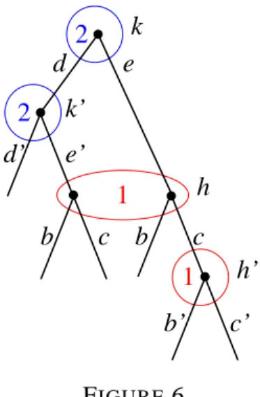
The example in Figure 6 demonstrates the two-part induction in the preceding proof. Player 1 has the information sets h and h0, and player 2 has k and k0. Except for h0 and k0, any two of these are connected. The sets of sequences of player 1 and 2 are S1= { /0, b, c, cb0, cc0} and S2 = { /0, d, e, dd0, de0}. Any non-empty sequence of player 2

has the reference sequence /0 of player 1, so that player 2’s move recommendations are generated first. For the sequences of player 1 that end in a move at h, the possible refer-ence sequrefer-ences are dd0, de0, or e. For the sequences that end in a move at h0, the reference sequences are d or e. That is, reference sequences can be “non-monotonic”, in the sense that “later” information sets (here h0, preceded by h) can have “shorter” reference se-quences (here d, which is a reference sequence forσh0c0, which is a proper prefix of the reference sequence dd0or de0for the sequenceσhc =σh0). For this reason, one needs the second, “inner” induction step (12) in the preceding proof, which amounts here to prov-ing thatµ(c, d) =µ(c, dd0) +µ(c, de0). In this example, all other cases of (11) involve a reference sequence directly, so that only the base case of the inner induction is required.

Figure 6 also demonstrates the use of reference sequences, and why it is useful to restrict z(σ,τ) to relevant sequence pairs. If one did not do the latter, one could specify probabilities z(cb0, dd0), z(cb0, de0), z(cc0, dd0), and z(cc0, de0) subject to (7), which cor-relate the moves at the two information sets h0 and k0. However, this correlation would not matter, but only the marginal probabilities z(cb0, d) and z(cc0, d) when player 2 has to