Mortgage life insurance:
a rationale for a time limit in switching rights
∗
Bertrand Villeneuve
Université Paris-Dauphine
June 24, 2014
Abstract
I examine competition in the sector of mortgage life insurance, in particular the Periodic Switching Right (PSR), by which the borrower can change his insurer once every period (say, every year). The PSR is likely to have pro competitive effects (lower premium), but by the same move, to lead to excessive segmentation. The main theoretical prediction of the PSR is that, in equilibrium, everyone will pay every year a premium reflecting his current risk, meaning that the risk of future risk evolution is not covered. This destruction of insurance is appreciated negatively by consumers. The trade-off is between, on the one hand, a lower price for insurance, and on the other hand, a lower quality of insurance. I simulate the cost of the PSR and find about 5%-15% of the total insurance cost. This order of magnitude is slightly smaller than the benefit one can expect from increased competition. All in all, a switching right limited in time would bring the benefits of competition and avoid most of the cost of segmentation.
Keywords: mortgage; life insurance; risk classification; regulation JEL classification codes: G22; G21; G18.
∗This study has been partly supported by the Ministère de l’économie et des finances (France). I thank Damien
Ientile and Olivier Taillardat for information and analysis. I also thank Céline Grislain-Letrémy and the referee for valuable suggestions. I am solely responsible for the opinions expressed in the text.
1
Introduction
In 2013, two opposite views emerged in France during the consultation of experts about the potential impact of a new switching right in the domain of mortgage life insurance. Some depicted it as destabilizing; others described it as a significant economic advance for consumers. The origin of the controversy is that the rates in this insurance line are clearly above actuarial rates, and often the double (BAO, 2013). This level of loading is certainly surprising given that the product is simple, standardized, and easy to monitor.1 A current perception was that
borrowers were essentially focused on loan rates, and they tended not to negotiate this part of the package. The idea is that, in practice, borrowers were not in a position to search efficiently for alternative insurance, perhaps for psychological reasons. The process is exhausting: finding a property, negotiating the price, signing an agreement with the seller, negotiating a loan rate, finalizing the purchase, all these demanding tasks leave little energy for optimizing mortgage life insurance. It seems that bankers take advantage of this state of spirit when they sell insurance. Legally, bankers are agents of independent insurance companies, and they receive commissions; the sharing of the loading between the insurer and the bank is a trade secret, but there are converging testimonies that bankers receive a significant proportion of the profit.
A first important move was the Loi Lagarde (Loi 210-737, 1st July 2010), that allowed borrowers, during a very short period after they received a firm loan proposal, to search for a so called “alternative insurer” rather than taking the so called “group insurance” proposed by the lending bank. This significant legal advance has not been a success in terms of the objectives pursued by the French government of the time. A vast majority of borrowers continued to subscribe group insurance, and more strikingly, rates charged did not decrease significantly, despite the development of much cheaper accessible alternative offers, but that were rarely chosen. Though understandable, this attitude of borrowers is hard to defend in economic terms: about 20%-25% of the lending cost goes to insurance. A more active search for cheaper insurance could save between a third and a half of this amount.
To go a step further, the French government examined in 2013 an extension of the duration of the insurance substitution right. This extension will be called PSR (Periodic Substitution Right) in this text. People cool off, and after a while, they are in better psychological and strategic position to negotiate insurance. Some argued that allowing substitution every year would be the most competitive solution. This view is taken by consumer rights association and consultancies in actuarial studies (BAO, 2013), the former, I will show, because they misunderstood the downside, and for the latter, maybe, because it meant more business for them (new products and more rating). Bankers were against, maybe because the current system is profitable, but some of them defended it by arguing that it performs a socially useful function, namely, cross subsidies between ages and risks (Durand, 2013; Cognat and de Villeneuve, 2013). Mortgage life insurance as, objectively, a subsidization of the old by the young, is a design I find hard to defend.
My contribution to this debate was and still is to show that the substitution right should be 1We can compare these fees with those found in another line of insurance, which is technically more complex, and
costlier to provide and monitor: health insurance. Karaca-Mandic et al. (2011) find a rate of about 35% for small groups of less than 100 workers; and much less for firms with larger groups of covered workers.
limited in time. This notion has been included in the Law (Loi 1014-344, 17th March 2014, Code de la consommation, Article L312-9). Admittedly, it is necessarily for improving the quality of competition in favor of consumers, but there is a (hidden) risk behind substitution rights, the risk that people cease completely to be insured against future discrimination. I characterize and quantify this risk in this paper.
Section 2 shows that the PSR for mortgage life insurance will produce, in equilibrium, complete segmentation every period. Section 3 poses evaluation principles of the PSR cost; a first numerical illustration is given. Section 4 gives an complete evaluation of the PSR of the whole duration of the loan. Policy implications are given in Section 5. Appendix A gives the code used for the simulations.
2
The periodic substitution right in mortgage life
in-surance
2.1
Facts about mortgage life insurance
Mortgage life insurance is paid by the borrower, it pays the lender the outstanding capital and interest in case the borrower dies. Other insured events like disability or unemployment are not considered in this study; Autorité de contrôle prudentiel (2013) gives information about regulation and practices for mortgages and related insurance.
The mortality risk being separately covered, it does not have to be included in the interest rate. The separability between the interest rate and the insurance justifies that the two could be supplied by two distinct financial entities: the lender and the insurer. The separation has been legal for long, but the commercial separation has been encouraged only recently in France, via the Loi Lagarde mentioned in the introduction. This bill allowed borrowers to choose freely their insurer, but once for all, and during a short time window after the loan is offered.
It has been observed that in practice, most people take the “group insurance” proposed by the bank, the bank being an agent for the insurer. A order a magnitude is 85% for group insurance in general, and significantly less for certain aggravated risks excluded given their medical records (BAO,2013). More intriguing, the cost of these insurance contracts are significantly higher than alternative ones borrowers could find in the market. Borrowers are clearly more sensitive to loan rate than to insurance rate. But insurance costs are not to be dismissed: insurance can cost as much as 25% of the full cost of the loan, i.e., about the double of what the actuarial premium would be.
Rates follow two types of principles (Cognat and de Villeneuve,2013). The most common principle is a constant premium based on the initial capital and age of the lender when he gets the loan. Note that since mortality increases and the outstanding capital decreases as time passes, the profitability is not constant over time. Indeed, the two above mentioned effects have contrary effects on the profitability. The other principle is to base the rate on the current outstanding capital, and insurance premia are periodically revised.
2.2
Full segmentation
I focus the analysis on equilibrium tariffs, i.e., tariffs that are consistent with competition given the PSR. In particular, the regulation may limit the rights to price discriminate. If no segmentation is allowed by the law, and if refusal to deal is also forbidden, the equilibrium is a single price if menus are not allowed either (Rothschild and Stiglitz,1976, and many other works citing this article). If only age can be taken into account, the equilibrium is an age-adjusted tariff.
Assume that discrimination is allowed, and that we are in a period, say, the second year, where borrowers can exert their PSR. In theory, all segmentation possibilities will be used, provided they bear statistical information on risk. This consequence can be proved by con-tradiction. All heterogeneous group (i.e., mixing different observable risks) treated equally by insurer A will experience cream-skimming. The best risks in the group are offered by insurer B better deals, which they accept. For example, insurer B can propose everyone a free analysis of the risk (e.g., medical records) and then make attractive offers to low risks thus detected. As such, the scheme is a good deal for borrowers, since they always keep the option to stay with their original insurer. But insurer A is left with the costly types, and he may enter in financial distress.
The key point is that insurer A must guarantee himself (and his customers) against cream-skimming. The only way to robustness is to adjust premia paid by borrowers to their observable risks period after period, either by decreasing or increasing the rate, depending on the evolution of the individual risk. This adjustment must be done even for those staying with the insurer. The threat of skimming have exactly the same theoretical consequences as actual cream-skimming. This logic goes as far as statistical discrimination can go, technically and legally. Any degree of heterogeneity, measurable with available and legal predictive techniques, in tariff classes is susceptible of cream-skimming. The equilibrium tariff is fully discriminating all the time: individual tariffs follow the trajectory of individual risk.
Claim 1. The PSR and competition will cause full discrimination every period.
This point is raised in several analyses of the PSR, though their practical conclusions and recommendations diverge. Durand (2013) says that even with imperfectly price sensitive con-sumers, the degree of segmentation will increase, with much higher prices for some groups. BAO(2013) insists that margins are so high that if competition eliminates them, all consumers, even the riskiest, will gain. With the same consequences in view, but with a totally different judgment, Cognat and de Villeneuve (2013) see “virtue” is the current system, because there are few classes (in particular in terms of age classes). This would be protective for the highest risks. This situation is not stable if competition is strong, even with the current regulation. Consumers could become unexpectedly more reactive to alternative insurers’ offers. In reality, segmentation possibilities are not all used. The reason could be the cost of segmentation; an-other more interesting explanation is that limiting segmentation can be a collusive scheme in an otherwise imperfectly competitive market. Little segmentation and comfortable profits suggest limited competition rather that virtue.
by all. The insurance literature sheds some light on this basic scenario by proposing important variations, adverse selection and excessive selection, that I examine in turn.
2.3
Adverse selection
Adverse selection relies on the assumption that there are relevant characteristics for risk that are observed by the insured, not the insurers (Rothschild and Stiglitz, 1976).2 Health is a good example: medical exams can overlook pathologies, or simply predispositions, known by the insured. Another important example is the characteristics observable by all but that the law forbids to use (e.g., under EU law, men and women, other things equal, must be treated equally, Cour de Justice de l’Union Européenne, 1st March 2011, Case C-236/09.).
Admittedly, insurers can sometimes use indirect selection means, like occupation, and any other variable correlated with risk-relevant forbidden traits. Other means, in particular self-selection via non-linear contracts, are used in practice and have been clarified by theorists. Insurers can offer menus of contracts, i.e., a well designed short list in which the insured can pick a contract. The list is conceived to provoke choices that are non neutral actuarially speaking. Ideally, the risky insured will tend to choose a certain type of contract and the less risky another type. Expensive contracts with a very good coverage are relatively more attractive than cheap contracts with limited coverage for the high risks. The price difference and the coverage difference have to be adjusted finely for the expected effect to work. Self-selection can be used to fight adverse selection.
Adverse selection is a dynamic phenomenon; it can be there in the first contract, but it can also emerge later if the insured learns or realizes something the insurers cannot observe. A borrower with good, privately known, genetic dispositions could search actively an alternative insurer. The PSR would facilitate this sort of moves.
The question of periodic revision of contracts has been developed by Cooper and Hayes (1987), in the case where both the insurer and the insured are definitely committed in the contract, and by Hosios and Peters (1989) and Dionne and Doherty(1994) in the case where the insured can unilaterally quit and get a better one (only the good type really poses a threat to do so). Dionne and Doherty(1994) study contract renegotiation. These articles do not focus on the notion of “type risk” I develop in this work.
2.4
Excessive selection
Excessive selection by insurers happens in the case where they base their tariffs on differences that the insured do not see. This phenomenon is described in Villeneuve (2005). In civil responsibility insurance, events are rare and consequences rather unforeseeable, especially if you consider the legal aspect. A better knowledge of the risk by insurers, through mastery of the jurisprudence, is plausible. The competition between insurers can be based on characteristics which the insured are not aware that they are relevant.
If competition is strong, the equilibrium segmentation will be entirely determined by the capacity to discriminate of insurers. Even the most ignorant insured is likely to be attracted 2A rich survey on adverse selection isDionne et al. (2000).
by the lowest price, no matter the actuarial reasoning behind it. Excessive selection is precisely a situation where actual selection overpasses risk perception by the insured, with detrimental effects.
Excessive selection is a serious threat. An individual insurer can find profitable to invest in better, new, segmentation criteria. They enable the insurer to pick profitable customers from unsuspecting competitors. They also enable the innovative insurer to discourage (which is more astute than plain refusal) bad risks via costly offers. The consequence is adverse selection for rival firms. But it is likely that will come a time when the practice becomes noticed by the pro-fession, and when it becomes generalized. Profits have been temporary, but the discrimination is installed. This erosion of profit may cause another round of innovation deepening again the degree of discrimination.
The limit of competitive segmentation are posed by the statistical prediction techniques, the test costs, and the decreasing size of groups as criteria are refined, so that finding new significant predictors becomes harder. However, these limits may be too loose for the society. Discrimination based on addresses, information on social networks, etc., are generally feared. Antidiscriminatory laws set limits, but their range is not universal. Another quite different issue is that blocking rating innovation may limit entry, and may facilitate collusion between incumbent insurers.
The insured suffer from this competitive race. Indeed people with the same (absence of risk) perceptions would find mutually advantageous to be pooled ex ante, rather than find themselves treated differently ex post. Risk aversion against this type risk makes people prefer no selection: otherwise, people see insurance prices as lottery tickets, and they would prefer a sure price for the same service. In any case, the PSR is likely to increase this effect. Every year will bring new segmentation, either because of truly novel techniques, or because of the application of existing ones to people, as they age and become increasingly different, statistically speaking.
Claim 2. In the long run, the PSR and competition lead to excessive competition.
Villeneuve(2005) shows that in a situation of excessive selection, collusion between insurers can happen. The right of insured not to be insured is at the basis of the reasoning. The idea is that an unusual offer by an deviant insurer can cause a drop in the customer’s willingness-to-pay for insurance; for example because he becomes very optimistic about his true risk. In that case, a deviant offer is accepted only if it is cheap, which may not be a better outcome for the insururer than to stay in the status quo. Note that there are multiple equilibria since the insured sees offers as signals, and signaling games often have multiple equilibria due to alternative rational beliefs players may have. This scenario may not be the most likely for mortgage life insurance, especially because these insurance are almost compulsory.3 Concerning explicit collusion, only detection and repression can work.
3
The cost of risk selection: a base case
3.1
A story
Would you prefer to know for sure that you will pay e1,000 for your insurance next year, or would you rather have 1/10 chance to pay e2,800 and 9/10 chance to pay e800? In terms of expectations, the two scenarios are identical. If you are risk averse, you prefer the former. But the latter is what will happen if tariffs are adjusted, year after year, to your current risk. Indeed, you could very well become ill (or at least you could show new disposition for severe illness), say with probability 1/10, and you would see the premium almost tripled. Unless you are lucky, and you will see a reduction of 20%. Definitely, you prefer the sure, average, e1,000. You would even be better paying a higher but guaranteed premium, rather than incurring the risk to win or lose, depending on health variations.
3.2
Cost
The cost considered here is not the cost to classify (which I neglect), but the social cost of classifying. I compare, for a borrower, the value of living in a world where he is treated like an average risk of his age whatever happens, with the value of living in a world where he pays for his current risk, in other words, of being in a world where the PSR is fully effective.
I define now the notion of “type risk”, i.e., the risk for the borrower to see his premium change randomly, as insurers revise periodically the risk classification of borrowers. It is a dynamic variety of the Hirshleifer effect (Hirshleifer, 1971; Crocker and Snow, 2000, for the notion that information can have negative private value); it has been discussed in the case of life insurance inVilleneuve (2000).
Year after year, dispositions to pathologies or long term affections appear. This evolution gives a basis for discrimination over time that deepens differences between people in unfore-seeable ways. In this view, the risk is a martingale. Aging is not the only factor driving risk classification over time. Scientific progress improves predictive medicine: the precisions of clinical, genetic and epidemiological predictors will increase. Though the speed at which they will change is unclear, it is very probable that the levels of segmentation they will allow are yet unseen (Crocker and Snow,1985, for basic modeling, andCrocker and Snow, 2000, for development).
To simplify, one can assume that at all age, people belong to one of two categories: aggravated risks (some pathology has come out) or attenuated risks (nothing noticeable). The mortality at a given age in standard tables is the mixture of the mortalities of the two groups.
Figure 1 illustrates what an individual of age t with attenuated risk sees of his immediate future (in the year to come): he will die with probability µt and he will live with the
com-plementary probability 1 − µt; conditional on his survival, his risk will stay attenuated with probability αt, or will pass to aggravated with probability 1 − αt.
In order to show the mechanism, an elementary simulation is given first. Section 4 gives complete results, comprising robustness tests on the less known parameters.
Consider an individual who estimates, at age t, his future utility when he is aged t + 1. The expected utility is calculated in two alternative scenarios. In the first scenario (UNI), insurers
Today After one year
Attenuated risk
at age t Attenuated riskat age t+1
Aggravated risk At age t+1 Death Transition probabilities μt (1 – μt)(1 – αt) (1 – μt) αt
Figure 1: Base case. µt: mortality between t et t + 1 ; αt: conditional probability to stay an
attenuated risk.
don’t discriminate and they charge the average price. In the second scenario (DIS), they charge a price adapted to the type the individual has; this scenario corresponds to what one expects from the PSR (Claim 1). In both scenarios, the expected insurance premium is exactly the same.
Scenario UNI (for uniform). The insurance premium charged at age t only depends on the
due capital and on the average risk. The premium is
λ µtKt,
where
• λ is the loading factor (λ = 1 would give the pure premium, λ = 2 gives the a good approximation of the prices charged for group insurance for one head). Source: price comparators, private communication.
• µt is the probability of death between ages t and t + 1. Source: INSEE.
• Kt is the outstanding capital, which serves as a basis for insurance.
Scenario DIS (for discrimination). The insurance premium charged at age t + 1 is random:
it corresponds either to the aggravated risk or to the attenuated risk, depending on what happens to the borrower (Figure1). The premium follows this dynamics
(
λ µtj Kt with probability αt,
λ µtg Kt with probability 1 − αt,
where
• αtis the probability that an attenuated risk at t remains an attenuated risk. • 1 − αt is the probability that an attenuated risk at t becomes an aggravated risk. • j is the risk attenuation factor: j < 1.
• g is the risk aggravation factor: g > 1.
the following relation:
µt= αtj µt+ (1 − αt) g µt ⇔ αtj + (1 − αt) g = 1.
The utility in scenario UNI is
UUNI= (1 − µt)U [W − Kt(r + λµt)] + µtU0, whereas the expected utility in scenario DIS is
UDIS = (1 − µt) (αtU [W − Kt(r + λjµt)] + (1 − αt) U [W − Kt(r + λgµt)]) + µtU0, where
• U [x] = x1−γ
1−γ is an isoelastic utility function with relative risk aversion γ. • U0 denotes the utility of the individual in case of death.
• W is the consumption during the year serving as a reference point for evaluating risk. • r is the interest rate of the loan. This value disappears from the calculations and has no
impact on the result for the reason that the two scenarios differ only in case of life, and probabilities are exogenous.
3.3
Sensitivity analysis
Because of risk aversion, we have UUNI > UDIS. To compare quantitatively the two cases, I calculate, for scenario UNI, the additional sure premium π that would make the expected utility equal to that of scenario DIS. So I search for π such that:
(1 − µt)U [W − Kt(r + λµt) − π] + µtU0 = UDIS, where risk aversion ensures that π > 0.
Base parameters. The values correspond to an average 55-year old borrower (mortality
rate 5 per thousand).
γ = 3; W = 50, 000 ; Kt= 100, 000 ; r = 3%; λ = 2; α = 0.9; µ = 0.5%; j = 0.555; g = 5.
Variations. Intervals for analyzed parameters:
γ ∈ [1, 3]; W ∈ [20, 000, 50, 000]; λ ∈ [1, 3]; α ∈ [0, 8, 1]; g ∈ [1.5, 5].
With the base scenario, the mortgage annual payment ise3,000, and the insurance premium in the UNI is e1,000. The value of π is to be compared with these e1,000. Figures 2 show parameter sensitivities of the risk premium, expressed ine per year.
A few comments on the figures. The set of simulations suggests a cost for the type risk due to segmentation of the order of 5% à 15% of the total cost of insurance. In the story given at
1.0 1.2 1.4 1.6 1.8 2.0 2.2 2.4 Γ 0 100 200 300 400 Equivalent cost HΕL 20 0000 25 000 30 000 35 000 40 000 45 000 50 000W 100 200 300 400 Equivalent cost HΕL Effect of γ Effect of W 0.800 0.85 0.90 0.95 1.00Α 100 200 300 400 Equivalent cost HΕL 2.0 2.5 3.0 3.5 4.0 4.5 5.0g 0 100 200 300 400 Equivalent cost HΕL Effect of α Effect of g 1.0 1.5 2.0 2.5 3.0Λ 0 100 200 300 400 Equivalent cost HΕL Effect of λ
the beginning of the section, that would mean that an individual would accept to pay as much as e1,150 for sure, rather than e1,000 in expectation. Increasing γ increases risk aversion: the cost of segmentation increases. The isoelastic utility function exhibits a risk aversion that decreases with the level of consumption W : the cost of discrimination is smaller for richer borrowers for the same installments; they can absorb risk more easily. The closer to 1 is α, the lower the probability to become an aggravated risk, which reduces the cost of risk. A higher aggravation factor g (a mean-preserving spread in fact) increases the cost of risk. The effect of the loading factor λ is strong, in particular because of the income effect: a higher λ cause higher installments, and the smaller consumption left to the borrower makes him more risk averse.
4
Evaluation over the whole duration of the loan
In this section, I calculate the cost of the segmentation risk over the duration of the loan. Empirically, one expects types to be rather persistent: aggravated risks tend to stay aggravated risks, or die; attenuated risks tend to stay attenuated risks. Trajectories could be relatively complex, as there is no compelling reason to assume that transition probabilities only depends on the current state rather that the whole history. In fact there is practically no actuarial literature on the dynamics of types. Fortunately, one can use Claim1 to affirm that, with the PSR, tariffs need not have memory.
As a proportion, the cost of the PSR is of the same order of magnitude as the one found for one year. Indeed, segmentation risks add up year after year, and do not compensate each other: securing people for one year do not change the valuation of the cost of segmentation for the other years. Technically, this additivity comes from the additive separability of the intertemporal utility function. To fix ideas, I limit the numerical illustration to a 15-year loan and the age span to 30-59 years (45 years for the older starting age).
One has to find or simulate: an intertemporal utility for comparison across scenarios; mortal-ity table over 30 years (from 30 to 59 year old); installment plan over 15 years (with amortization and insurance), given that the tariff depends on the outstanding capital; a distribution of types over 30 years.
Notation: • U (c) = c1−γ
1−γ the utility function for a year (isoelastic with coefficient of relative risk aversion γ; base scenario: γ = 2.5).
• U0 utility in case of death (arbitrarily set to 0 without loss of generality). • β the discount factor for future utility (β = 0.97).
• a age when the loan starts (a between 30 and 45, depending on scenario).
• Wt consumption at age t, before accounting for mortgage installment and insurance (growth rate of 2% per year, starting point W30= 25, 000 in the base scenario).
• K borrowed capital (e100,000 in the base scenario); r loan rate (r = 3%); A = r K(1+r)(1+r)1515−1
constant installment over 15 years; Kt= K(1+r)
15−(1+r)t−a
(1+r)15−1 outstanding capital at age t.
• µt mortality rate before age t + 1 for those living at age t; Stsurvival probability at age t
• αt proportion of attenuated risks at age t; 1 − αtproportion of aggravated risks at age t.
• gt > 1 risk aggravation factor at age t (base scenario: gt = 3); jt < 1 risk attenuation
factor at age t, calculated given that αtjt+ (1 − αt)gt= 1.
• λ insurance loading factor (base scenario λ = 2).
Specific assumptions and parameter choice. At age a, there is no installment, only
insurance; at age a + 15, the last installment is paid, but no insurance (Ka+15= 0).
Aggravation and attenuation factors are critical parameters on which we have little infor-mation. I have explored for g the interval [1, 7], which is quite large. The effect of g is almost quadratic, because it’s increase represents mean-preserving spread of so called type risk. The proportion of aggravated risk in the population is assumed to increase linearly with age.
Kocherlakota(1996) discusses the admissible values for the coefficient of relative risk aversion
γ. The answer is a large range, and more important, the effect is practically linear. What is
interesting for my research objective is that even at low values of γ, the cost of the PSR is significant, and all the more so as γ increases.
Utility without discrimination (UNI):
VUni=SaU [Wa− λ µaK] + (1 − Sa) U0+
s=15
X
s=1
βs × {Sa+sU [Wa+s− A − λ µa+sKa+s] + (1 − Sa+s) U0} .
Utility with discrimination (DIS):
VDis =SaU [Wa− λ µaK] + (1 − Sa) U0+
s=15
X
s=1
βs× { Sa+s(αa+sU [Wa+s− A − λ ja+sµa+sKa+s]
+ (1 − αa+s) U [Wa+s− A − λ ga+sµa+sKa+s])
+ (1 − Sa+s) U0} .
The concavity of the utility function provides Jensen’s inequality, VUni> VDis. Let’s search, in scenario UNI, the maximum extra loading rate τ on the premium that would leave this riskless situation preferred to scenario DIS. Formally, τ is such that:
SaU [Wa− λ (1 + τ )µaK] + (1 − Sa) U0+
s=15
X
s=1
βs × {Sa+sU [Wa+s− A − λ (1 + τ ) µa+sKa+s] + (1 − Sa+s) U0} = VDis.
The figures show τ in various cases. Remark that there are alternative interpretations of 1 + τ . It can be seen as a proportional increase of mortality as perceived (and charged) by insurers; it can also be seen as a proportional increase of outstanding capital.
install-of the model to the parameters. The most critical parameters are the risk aversion γ and the risk factor g. 35 40 45 50 55 60 0.2 0.4 0.6 0.8 1.0
Figure 3: Survival probability (top) and probability to be an aggravated risk (bottom) depending on age. For the living at age 30.
46 48 50 52 54 56 58 60
2000 4000 6000 8000
Figure 4: Annuity (top), interest on outstanding capital (middle) and insurance (bottom) depending on age. Loan at age 45.
Overall, I find an evaluation of the cost of the type risk at 5-10 % of the total cost of insurance. Note it could be seen as a lower bound, because future segmentation can be seen as unfamiliar, uncertainty, or ambiguous (to use a few terms in non expected utility analysis).
5
Policy implications
What could happen if a new PSR were introduced in the market for mortgage life insurance?
Ongoing contracts. Unbinding one of the parties (i.e., borrowers) would certainly
destabi-lize the market. Whether this is constitutional is doubtful, but this is not the point raised here. Insurer A would suffer from the fact that insurer B would pick the best of insurer A’s clients.
1.5 2.0 2.5 3.0 3.5Γ 0 5 10 15 20 Equivalent cost H%L 20 0000 22 000 24 000 26 000 28 000 30 000W30 5 10 15 20 Equivalent cost H%L Effect of γ Effect of W 1 2 3 4 5 6 7g 0 5 10 15 20 Equivalent cost H%L 1.5 2.0 2.5 3.0 3.5 4.0 4.5 5.0Λ 0 5 10 15 20 Equivalent cost H%L Effect of g Effect of λ
Figure 5: Segmentation cost sensitivity. Loan subscription at age 45.
30 32 34 36 38 40 42 44 Age 0 1 2 3 4 5 6 7 Equivalent cost H%L
The main problem is that the effect would not be actuarially neutral, on the contrary it would aggravate adverse selection on previous deals. The error would be to see only the lower prices, and to interpret them as an only beneficial fruit of competition.
Contracts could be renegotiated, but this is never is the interest of both parties. Any renego-tiation would imply increasing or decreasing the premium depending on new risk classification; at least one of the parties would oppose a price change. This effect comes from the fact that insurance is ex ante and ex post optimal, a result that competition under normal conditions should yield.4
New contracts. With the PSR, all new contracts will internalize the risk of cream-skimming.
To do so, the only solution is to plan a periodic resegmentation of the insured. The segmentation will go as far as statistical methods can go. The notions of high and low risks often used in this literature are useful simplifications (Rothschild and Stiglitz, 1976; Villeneuve, 2003); the important fact is that any class of risk can be subdivided until statisticians reach the limits of their discriminatory abilities. Strictly speaking, the market is not destabilized; it works on a new basis.
The reasoning behind the prediction of full segmentation supposes that the insured are sensitive to price differences. Such an assumption seems natural, however there is evidence in numerous sectors (banks, telecoms, healthcare) that people tend to limit search for better deals even if this strategy is profitable. Many consumers are quite passive. With public prices, they may simply free-ride on active consumers; with personalized prices as with life insurance, passivity is likely to be less efficient. Insurers could identify passive policyholders, and strategies to attract them (low-balling for example) could be be used against them.
The question that follows would be: do they suffer (indirectly but definitely) from the PSR as it is used by active peers? Indeed, passive good risks would consent, by their passivity, to subsidies bad risks. Insurance prices may not be as private as they used to be: it has become relatively simple to collect information on Internet platforms to document firms’ behaviors. The cost of gathering from the public, and diffusing among them, information has decreased. This situation is likely to benefit even the most passive customers.
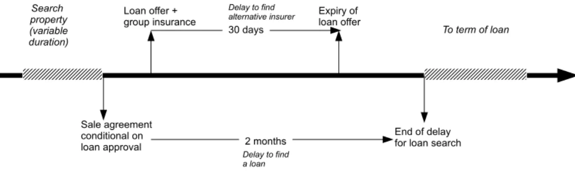
Limiting the PSR. Finding a property, then a loan, then an alternative insurer (Figure 7)
entails some risk at each stage that hinders effective competition between insurers, especially because insurance is the last and smallest step. Lenders have interest to delay as much as possible the formalization of their offer, or the examination of alternative insurance contracts, to limit the time available to borrowers in their final search for insurance. It is common practice in France (in preliminary sales agreement) to have to pay 10% of the value of the property if one renounces to the purchase for reasons other than plain loan refusal. This ultimatum biases insurance pricing, more than it biases interest rates, because borrower spend their energy on the latter, though competition on loans only work reasonably well. The legal information facilitates comparisons, and the public is generally well educated in this aspect of property acquisition.
Insurance in contrast is a rather discreet place where to earn comfortable margins. Indeed, 4Bolton and Dewatripont(2005) for a complete synthesis on contract theory, and the effect of commitment to reach
Search property (variable duration) Sale agreement conditional on loan approval Delay to find alternative insurer To term of loan Loan offer + group insurance End of delay for loan search
Delay to find a loan 2 months 30 days Expiry of loan offer
Figure 7: Steps for mortgage financed property acquisition.
banks are remunerated as agents of insurance companies, in a completely opaque way. It is now largely admitted in personal finance issues that protocol and default options matter (Sunstein and Thaler,2008). Leaving group insurance as the default choice leave too much local market power to lenders. A substitution right limited in time, but significantly longer than in the current system (30 days) is a possible solution. The analysis shows the cost of the PSR. What are the benefits? In theory, the substitution right does not have to be open during a large window to be effective and provide competitive effects. One has to admit that the exhausting steps towards a loan fragilize people’s ability to negotiate serenely their mortgage life insurance contracts.
We have seen that the PSR over the duration of the loan is not a good idea, so limiting the duration during which substitution is possible is a sensible option. A suggestion is to keep it to 6 months or 1 year at most. This duration contains strictly the risk of resegmentation and it seems a reasonable time for people to reconsider they borrowing strategy, especially their mortgage life insurance
How will we see that it has worked? As the theory of contestable markets have made clear (Baumol et al.,1982), the proportion of borrowers turning to alternative insurers is not a clear signal. The analysis of insurance prices is a much more reliable indication of effective competition: observing the evolution of the ratio between insurance rates and mortality rates will be easy and informative.
In any case, facilitating their development is recommendable: the product is not extremely sophisticated, comparisons between offers is easy. The barriers to entry were essentially in the timing of insurance sales; technical dimensions are minor. Therefore the market is very likely to be made contestable by a limited PSR.
References
Autorité de contrôle prudentiel (2013). Le financement de l’habitat en 2012. Banque de France, Paris.
BAO (2013). Assurance emprunteur immobilier: étude d’impact de l’application effective de la résiliation annuelle. http://www.baofrance.com/telechargement/Etude_impact_r%C3% A9siliation_25%20avril%202013.pdf.
Baumol, W., Panzar, J., and Willig, R. (1982). Contestable markets and the theory of industry
structure. Harcourt Brace Jovanovich, New York.
Bolton, P. and Dewatripont, M. (2005). Contract theory. MIT Press.
Cognat, D. and de Villeneuve, P. (2013). Les vertus sociales de l’assurance des emprunteurs.
Risques, 94:36–42.
Cooper, R. and Hayes, B. (1987). Multi-period insurance contracts. International Journal of
Industrial Organization, 5:211–231.
Crocker, K. J. and Snow, A. (1985). The efficiency of competitive equilibria in insurance economics with adverse selection. Journal of Public Economics, 26:207–219.
Crocker, K. J. and Snow, A. (2000). Handbook of Insurance, chapter The Theory of Risk
Classification, pages 245–276. Kluwer Academic Publishers.
Dionne, G. and Doherty, N. (1994). Adverse selection, commitment and renegotiation with application to insurance markets. Journal of Political Economy, 102:209–235.
Dionne, G., Doherty, N., and Fombaron, N. (2000). Handbook of Insurance, chapter Adverse Selection in Insurance Markets, pages 186–243. Kluwer Academic Publishers.
Durand, R. (2013). Etude « assurance des emprunteurs » collectives et individuelles.
ACTU-ARIS International.
Hirshleifer, J. (1971). The private and social value of information and the reward to inventive activity. American Economic Review, 61:561–574.
Hosios, A. J. and Peters, M. (1989). Repeated insurance contracts with adverse selection and limited commitment. Quarterly Journal of Economics, 104:229–253.
Karaca-Mandic, P., Abraham, J. M., and Phelps, C. E. (2011). How do health insurance loading fees vary by group size?: implications for healthcare reform. International Journal of Health
Care Finance and Economics, 11:181–207.
Kocherlakota, N. (1996). The equity premium: It’s still a puzzle. Journal of Economic
Litera-ture, 34:42–71.
Rothschild, M. and Stiglitz, J. E. (1976). Equilibrium in competitive insurance markets: An essay on the economics of imperfect information. Quarterly Journal of Economics, 90(4):630– 649.
Sunstein, C. R. and Thaler, R. H. (2008). Nudge. Yale University Press.
Villeneuve, B. (2000). Handbook of Insurance, chapter Life insurance, pages 902–931. Kluwer Academic Publishers.
Villeneuve, B. (2003). Mandatory pensions and the intensity of adverse selection in life insurance markets. Journal of Risk and Insurance, 70(3):527–548.
Villeneuve, B. (2005). Competition between insurers with superior information. European Economic Review, 49:321–340.
A
Code used for simulations
Mathematica code for the referee’s information. It will be removed from the paper for publi-R cation but it will be made available on my personal website.
(* Utility function *) U@x_D:= x ^H1- ΓLH1- ΓL; (* Notation Discount factor: Β Consumption: W[t] Outstanding capital: K Interest rate: r Loading factor: Λ *) (*
Parameters relevant for loan duration
Survival probability between t and t+1 : 1 - Μ[t] Conditional of survival
probability of attenuated risk Α[t] probability of aggravated risk 1 - Α[t]
Attenuation factor: j < 1 Aggravation factor: g > 1 *) (* Cost of insurance UNI a = Λ Μ DIS a = Λ j Μ with probability Α a = Λ g Μ with probability 1 - Α *) (* Mortality tables
Ages groups: 30-59 (30 years) by 5-year groups Rates: 0.7 ; 1.0 ; 1.5 ; 2.5 ; 4.1 ; 6.0 (per thousand) *) BaseMortalityIned =80.7, 1, 1.5, 2.5, 4.1, 6<; Do@Μ@tD =BaseMortalityIned@@1DD 1000,8t, 30, 34<D; Do@Μ@tD =BaseMortalityIned@@2DD 1000,8t, 35, 39<D; Do@Μ@tD =BaseMortalityIned@@3DD 1000,8t, 40, 44<D; Do@Μ@tD =BaseMortalityIned@@4DD 1000,8t, 45, 49<D; Do@Μ@tD =BaseMortalityIned@@5DD 1000,8t, 50, 54<D; Do@Μ@tD =BaseMortalityIned@@6DD 1000,8t, 55, 59<D; DiscretePlot@Μ@tD,8t, 30, 59<D 35 40 45 50 55 0.001 0.002 0.003 0.004 0.005 0.006
(* Smoothing at year level *)
Do@Μ@tD =BaseMortalityIned@@1DD 1000 *H1.07 ^Ht-32LL,8t, 30, 34<D; Do@Μ@tD =BaseMortalityIned@@2DD 1000*H1.07 ^Ht-37LL,8t, 35, 39<D; Do@Μ@tD =BaseMortalityIned@@3DD 1000*H1.09 ^Ht-42LL,8t, 40, 44<D; Do@Μ@tD =BaseMortalityIned@@4DD 1000*H1.11 ^Ht-47LL,8t, 45, 49<D; Do@Μ@tD =BaseMortalityIned@@5DD 1000*H1.09 ^Ht-52LL,8t, 50, 54<D; Do@Μ@tD =BaseMortalityIned@@6DD 1000*H1.07 ^Ht-57LL,8t, 55, 60<D; DiscretePlot@Μ@tD,8t, 30, 60<D DiscretePlot@Log@Μ@tDD,8t, 30, 60<D 35 40 45 50 55 60 0.001 0.002 0.003 0.004 0.005 0.006 0.007 35 40 45 50 55 60 -7.0 -6.5 -6.0 -5.5 -5.0
(* Survival probability at age t (for the living at age 30) *)
S@30D = H1- Μ@30DL; Do@S@t+1D =S@tD H1- Μ@tDL,8t, 30, 59<D; DiscretePlot@S@tD,8t, 30, 60<D 35 40 45 50 55 60 0.93 0.94 0.95 0.96 0.97 0.98 0.99 1.00 (*
Table for attenuated and aggravated risks: proportion of aggravated risk increasing from 8 % to 15 % *)
Α@t_D =1- Α0H.15 +Ht-30L.005L; DiscretePlot@Α@tD . Α0®1,8t, 30, 60<D 35 40 45 50 55 60 0.72 0.74 0.76 0.78 0.80 0.82 0.84
(* Survival as an aggravated risk, survival *)
DiscretePlot@8S@tD H1- Α@tDL, S@tD< . BaseRule,8t, 30, 60<D 35 40 45 50 55 60 0.2 0.4 0.6 0.8 1.0
(* Aggravation and attenuation factors: exploitation of restriction between parameters *)
EqMortality@t_D = Α@tDj + H1- Α@tDLg == 1;
j@t_D = j . Solve@EqMortality@tD, jD@@1, 1DD;
(* Annuity (without insurance) and outstanding capital *)
A =r KH1-H1+rL^H-nLL;
K@p_D =KHH1+rL^ n-H1+rL^ pLHH1+rL^ n-1L;
(* Installment table; interest; insurance *)
Risque_typage-2014-04-28.nb 3
BaseRule = 8Γ ®3,Β ®0.97, W30®25 000, K®100 000, r®.03, g®3,Λ ®4, n®15,Α0®1<; DiscretePlot@ 8A, K@t-45Dr, ΛK@t-45D Μ@tD < . BaseRule,8t, 45, 60<D 46 48 50 52 54 56 58 60 2000 4000 6000 8000
(* Amortization (top); insurance premium (bottom) *)
DiscretePlot@ 8K@t-30Dr, K@t-30D Μ@tD < . BaseRule,8t, 30, 45<D 32 34 36 38 40 42 44 500 1000 1500 2000 2500 3000 (* Income *) W@t_D =W30H1.02L^Ht -30L; DiscretePlot@W@tD . W30®25 000,8t, 30, 45<D 32 34 36 38 40 42 44 26 000 28 000 30 000 32 000
(* P is the fictious proportional charge equalizing utilities in both scenarios *) (* Function for age a at start *)
U0 =0; Uunia = SumBΒ^HsL S@a+sDH W@a+sD -A - K@sD Λ Μ@a+sD H1+PLL1-Γ 1- Γ +H1-S@a+sDLU0 ,8s, 1, 15<F; Udisa =SumBΒ^HsL S@a+sD Α@a+sDH W@a+sD -A -K@sD Λj@a+sD Μ@a+sD L1-Γ 1- Γ + H1- Α@a+sDLH W@a+sD -A -K@sD ΛgΜ@a+sD L1-Γ 1- Γ +H1-S@a+sDLU0 ,8s, 1, 15<F ;
(* Parameter lists, each being free in turn *)
BaseRule = 8Γ ®3,Β ®0.97, W30®25 000, K®100 000, r®.03, g®3,Λ ®4, n®15,Α0®1<; GammaRule = 8 Β ®0.97, W30®25 000, K®100 000, r®.03, g®3,Λ ®4, n®15,Α0®1<; WRule = 8Γ ®3,Β ®0.97, K®100 000, r®.03, g®3,Λ ®4, n®15,Α0®1<; AlphaRule = 8Γ ®3,Β ®0.97, W30®25 000, K®100 000, r®.03, g®3,Λ ®4, n®15 <; GRule = 8Γ ®3,Β ®0.97, W30®25 000, K®100 000, r®.03, Λ ®4, n®15,Α0®1<; LambdaRule =8Γ ®3,Β ®0.97, W30®25 000, K®100 000, r®.03, g®3, n®15,Α0®1<;
(* P as of function of free parameter (one function per free parameter) *)
GammaPrimeT@z_, x_D:=P . FindRoot@Uunia==Udisa . GammaRule . Γ ®z. a®x,8P, 0, 1<D;
WPrimeT@z_, x_D := P . FindRoot@Uunia==Udisa . WRule . W30®z. a®x,8P, 0, 1<D;
AlphaPrimeT@z_, x_D:=P . FindRoot@Uunia==Udisa . AlphaRule . Α0®z . a®x,8P, 0, 1<D;
GPrimeT@z_, x_D := P . FindRoot@Uunia==Udisa . GRule . g®z. a®x,8P, 0, 1<D;
LambdaPrimeT@z_, x_D:= P . FindRoot@Uunia==Udisa. LambdaRule . Λ ®z. a®x,8P, 0, 1<D;
(* Figures *)
Plot@GammaPrimeT@Γ, 45D *100,8Γ, 1.5, 3.5<,
PlotRange®881.5, 3.5<,80, 20<<, AxesLabel®8Γ, "Equivalent cost H%L"<D
Plot@WPrimeT@W, 45D *100,8W, 20 000, 30 000<, PlotRange®8820 000, 30 000<,80, 20<<,
AxesLabel®8W30, "Equivalent cost H%L"<D
Plot@AlphaPrimeT@Α, 45D *100,8Α, 1, 1.5<, PlotRange®881, 1.5<,80, 20<<,
AxesLabel®8Α, "Equivalent cost H%L"<D
Plot@GPrimeT@g, 45D *100,8g, 1, 7<, PlotRange®881, 7<,80, 20<<,
AxesLabel®8g, "Equivalent cost H%L"<D
Plot@LambdaPrimeT@Λ, 45D *100,8Λ, 1.5, 5<, PlotRange®881.5, 5<,80, 20<<,
AxesLabel®8Λ, "Equivalent cost H%L"<D
1.5 2.0 2.5 3.0 3.5 Γ 0 5 10 15 20 Equivalent costH%L Risque_typage-2014-04-28.nb 5 23
20 000 22 000 24 000 26 000 28 000 30 000 W30 0 5 10 15 20 Equivalent costH%L 1.0 1.1 1.2 1.3 1.4 1.5Α 0 5 10 15 20 Equivalent costH%L 1 2 3 4 5 6 7 g 0 5 10 15 20 Equivalent costH%L 1.5 2.0 2.5 3.0 3.5 4.0 4.5 5.0 Λ 0 5 10 15 20 Equivalent costH%L
(* Other figures: sensitivity on age at loan subscription *) 6 Risque_typage-2014-04-28.nb
DiscretePlot@GammaPrimeT@3, aD *100,8a, 30, 45<,
PlotRange®8830, 45<,80, 7<<, AxesLabel®8"Age", "Equivalent cost H%L"<D
30 32 34 36 38 40 42 44 Age 0 1 2 3 4 5 6 7 Equivalent costH%L Risque_typage-2014-04-28.nb 7 25