Precautionary principle and the cost benefit analysis of innovative projects

HAL Id: hal-00570317

https://hal.archives-ouvertes.fr/hal-00570317

Preprint submitted on 28 Feb 2011

HAL is a multi-disciplinary open access archive for the deposit and dissemination of sci-entific research documents, whether they are pub-lished or not. The documents may come from teaching and research institutions in France or abroad, or from public or private research centers.

L’archive ouverte pluridisciplinaire HAL, est destinée au dépôt et à la diffusion de documents scientifiques de niveau recherche, publiés ou non, émanant des établissements d’enseignement et de recherche français ou étrangers, des laboratoires publics ou privés.

Precautionary principle and the cost benefit analysis of

innovative projects

Marc Baudry

To cite this version:

Marc Baudry. Precautionary principle and the cost benefit analysis of innovative projects. 2011. �hal-00570317�

EA 4272

Precautionary principle

and the cost benefit analysis

of innovative projects

Marc Baudry *

2011/06

* LEMNA : Université de Nantes

Laboratoire d’Economie et de Management Nantes-Atlantique Université de Nantes

Chemin de la Censive du Tertre – BP 52231

D

o

cu

m

en

t

d

e

T

ra

va

il

W

o

rk

in

g

P

ap

er

PRECAUTIONARY PRINCIPLE AND THE COST BENEFIT ANALYSIS OF INNOVATIVE PROJECTS

Marc Baudry

Université de Nantes – IEMN-IAE & LEMNA Address :

Chemin de la Censive du Tertre - BP 52231 44322 NANTES Cedex 3

France

email : marc.baudry@univ-nantes.fr

tel: +33.2.40.14.17.05

Abstract : Public authorities often invoke the precautionary principle to ban or postpone the development of innovative projects with uncertain but potentially harmful irreversible impacts on the environment or health. As stated in the Rio declaration, the precautionary principle suggests balancing costs and benefits associated with irreversible decisions while taking account of the perspective to acquire better but costly information in the future. Though the real option theory seems to be an appropriate tool to deal with the precautionary principle it has two important limits with this respect. First it focuses on Markovian processes rather than on Bayesian learning. Second, it disregards the role of preferences whereas preferences are at the core of the seemingly linked concept of precautionary saving. The article is an attempt to circumvent these two limits. A canonical model of Bayesian real option expressed in terms of intertemporal utility maximisation is presented and solved. The optimal decision rule is discussed in the light of the precautionary principle. It is then shown how to switch consistently to an equivalent problem expressed in terms of costs and benefits. JEL classification :. Q55, D81, C61.

Key words : Precautionary principle, Real options, Bayesian learning, Environmental preservation, Irreversibility, Uncertainty.

PRECAUTIONARY PRINCIPLE AND THE COST BENEFIT ANALYSIS OF INNOVATIVE PROJECTS

1.INTRODUCTION

Implications from the use of new technologies are often ambivalent. On the one hand new technologies are by essence intended to satisfy human needs and, as such, they generate benefits. On the other hand, unforeseen effects on the environment and health may appear. Impacts on the environment associated to the use of Genetically Modified Organism in agriculture or consequences on health of the use of cellular phones are among the most often quoted and analysed examples. Facing the decision whether to allow or ban new technologies in the presence of suspicions of harmful effects on the environment and/or health, public authorities in Europe generally invoke the precautionary principle to argue in favour of a, at least temporary, ban. The precautionary principle they referred to is that defined at the earth summit that took place at Rio de Janeiro in 1992. Indeed, principle fifteen of Rio declaration states that “Where there are threats of serious or irreversible damage, lack of full scientific

certainty shall not be used as a reason for postponing cost-effective measures to prevent environmental degradation”1. Similar definitions have been enacted in other national or international laws (see Gollier 2001 or Immordino 2003). From an economist point of view there are three key concepts embedded in the Rio conference definition. The first key concept is that of irreversibility. If damages were not irreversible, inappropriate decisions could be corrected and associated costs could be avoided thanks to a feedback effect. Irreversibility makes such a correction ineffective and thus strengthens the effects of an inappropriate decision. The second key concept is that of a lack of full scientific certainty. Scientific knowledge is not exogenous but cumulates through time as the result of a costly research activity. Thus the first two key concepts call for a dynamic approach to the precautionary principle. The third key concept is that of cost-effectiveness. It implicitly means public authorities have to balance costs and benefits. Surprisingly, how to balance costs and benefits in the presence of potential irreversible harmful effects and scientific evolving knowledge is not much detailed in the economic literature.

Since the seminal articles by Arrow and Fisher (1974) and Henry (1974) and the clarification made by Hanemann (1989), economists generally invoke the “irreversibility effect” to explain that the more uncertain we are about future returns from an irreversible project, the more the postponement of the project is relevant. The “irreversibility effect” has received much attention due to the ability to implement it to irreversible investment choices

1

Full text of the Rio declaration was available in February 2011 at

thanks to the real option theory synthesized in the now well known articles and textbook by Pindyck (1991), Dixit (1992), and Dixit and Pindyck (1994). Although the real option theory is originally build on a comparison with financial options (see, for instance, the pioneering works of McDonald and Siegel 1986 or Brennan and Schwartz 1985), its relationship with the concept of options and the “irreversibility effect” originally developed and clarified by Arrow Fisher Henry and Hanemann (AFHH) has been outlined, among others, by Lund (1991) and Fisher (2000). The real option theory is commonly quoted in works dealing with the precautionary principle but it has never been applied, to our knowledge, to explicitly model it. We suggest two ways to explain this paradox.

First, as noted by Ulph and Ulph (1997), assumptions about stochastic variables made in the real option theory are not appropriate for a wide range of economic problems implying both irreversibility and uncertainty. The reason for this is that the real option theory focuses on problems where independent exogenous and repeated shocks affect the evolution of a key variable in the decision of whether to develop or postpone an irreversible project. This approach, thereafter called Markovian approach, is relevant to deal with uncertainty affecting future prices but it is not suitable to deal with uncertainty about an unknown parameter, the true value of which is invariant with time. The latter kind of problems entails an analysis in terms of Bayesian uncertainty. The matter is that, in its primary version, the concept of option introduced by Arrow and Fisher (1974) is sufficiently large to be thought of as a problem with either Markovian uncertainty or Bayesian uncertainty while the reference to a learning process and Bayesian uncertainty is made more explicit in the subsequent literature. Fisher and Hanemann (1987) and Hanemann (1989), for instance, explicitly refer to Bayesian uncertainty when focusing on uncertainty about biological and engineering parameters or uncertainty as to whether the offshore structures contain oil in commercial quantities. By contrast, the analysis of the optimal timing of environmental policies proposed by Pindyck (2000) still refers to Markovian uncertainty.

Second, economists often have other theoretical references than the real option theory in mind when dealing with the precautionary principle. Indeed, precautionary saving is a well known and extensively concept in macroeconomic dynamics. For many economists, adapting the concept of precautionary saving to environmental policies thus seems to be a natural way to analyse the precautionary principle. One of the most noticeable articles that obey to this logic is that by Gollier et al. (2000). As a result, preferences, and more specifically attitude toward risk, play a crucial role in determining whether the precautionary principle is theoretically founded or not. This contrasts with the real option theory that may be thought of as an advanced Costs Benefits Analysis method specified in terms of monetary units without explicit reference to the concept of utility. The fact that models adapted from the concept of precautionary saving focuses on continuous choices in a macroeconomic context rather than discrete choices in a microeconomic context adds to the gap with the real option theory.

Nevertheless, citations of Dixit and Pindyck (1994), considered as the core of the real options literature, are still made in works building on the concept of precautionary saving (and more specifically in the article by Gollier et al. 2000).

This article is an attempt to unify the different ways suggested to analyse the precautionary principle. It starts with a Bayesian approach to the dynamics of scientific knowledge and highlights the role of prior beliefs in the debate about the precautionary principle and the importance to accord to the arrival of new information (section 2). We then turn to the presentation of a canonical model of Bayesian real option expressed in terms of intertemporal utility maximisation (section 3). The optimal exercise rule of the option helps identifying rules to balance advantages and disadvantages when facing a discrete choice with irreversible but uncertain impacts. These rules are used as a guideline to characterise cost effectiveness in the precautionary principle (section 4). For this purpose, a reformulation of the canonical Bayesian real option model is proposed in the specific case of a project with marginal impact. We more specifically focus on how to switch consistently from a specification in terms of utility to a specification in terms of monetary values.

2.A DYNAMIC APPROACH TO SCIENTIFIC UNCERTAINTY

This section introduces a Bayesian representation of the dynamics of scientific knowledge. How to model in a simple setting the arrival of informative but noisy messages about potential harmful effects of a project is first examined (2.1). We then turn to a discussion of decision errors and illustrate it with the case of a risk of dissemination of Genetically Modified Organisms (GMOs) in agriculture (2.2). We also examine in what respect the basic model proposed by Arrow and Fisher (1974) introduces some confusion between Markovian and Bayesian approaches to uncertainty.

2.1Bayesian learning and scientific progress

Since the seminal article of Arrow and Fisher (1974), the prospect of an arrival of new information is the core of the analysis of irreversible economic decisions. New information takes either the form of the observation of exogenous random shocks (described as Markov processes) affecting the evolution of some key variables or the form of messages used to revise the beliefs of economic agents. The real option theory typically focuses on the first representation of information while the work of AFHH and, more especially, the subsequent literature is merely influenced by the second representation. This second representation constitutes the basis for modelling scientific uncertainty as regards the irreversible consequences of developing an innovative project. It is generally assumed that there is a finite set of possible values of the unknown parameter and that there exists an a priori, or subjective, discrete probability distribution on this set representing the beliefs about the true

value of the unknown parameter. Messages arriving with time are used to revise the probability distribution. Some basic or intuitive properties of the revision process are expected. First of all, uncertainty decreases in the long term. This means that the probability for one of the possible values tends to increase with time while the probability assigned to other values tend to decrease. Some authors rule out the eventuality of contradictory messages, which allows representing the evolution of knowledge as an information structure which becomes finest as time goes2. As a result, the evolution of probabilities assigned to the different possible values of the unknown parameter is monotonic. If the eventuality of contradictory or noisy messages arriving at different dates is not ruled out, the evolution of probabilities is not monotonic: it may be the case that a probability increases and then decreases on two successive periods of time. Kolstad (1996a) for instance takes account of such noisy messages. Then, the evolution of probabilities may be viewed as a stochastic process with an attractor corresponding to a vector made of zeros except one of its components (that associated to the correct value of the unknown parameter) equal to unity. Another important property of the evolution of beliefs is that the revision of probabilities may be consistent with the probability theory, more especially with Bayes’ theorem. This point has not always received attention in the literature dealing with irreversible decision when facing uncertainty. A noticeable exception is the article by Kelly and Kolstad (1999). Though their model is not formalised in terms of real options, it has set the intuition for our canonical model.

Consider an innovative project intended to generate an additional flow of revenues for all future dates. Nevertheless, there are threats that developing the project generates irreversible though uncertain damages. Uncertainty affects damages in the sense that two scenarios are envisaged. The optimistic scenario refers to the case where the development of the project does not generate damages and, conversely, the pessimistic scenario refers to the case where the development of the project generates damages. Whether damages are generated by the project or not is known with certainty only once the project is developed. Before the project is developed, economic agents have beliefs about what is the correct scenario. Beliefs are based on common and public but costly information. C denotes the deterministic flow of investigation costs that has to be incurred on one unit of time to eventually receive additional information with probability 1 where is the probability that the investigation yields no new result. Investigation costs are expressed in terms of consumption units. Probability of receiving additional information on one period of time for a given investigation cost C may be thought of as a rough measure of the speed of knowledge acquisition. Due to the arrival of information through time, beliefs are nor static but dynamic. Beliefs are represented by subjective probabilities associated to each scenario.

2

This is typically the case in Freixas and Laffont(1984) or Kolstad(1996b) who merely follow the primary model of Henry(1974).

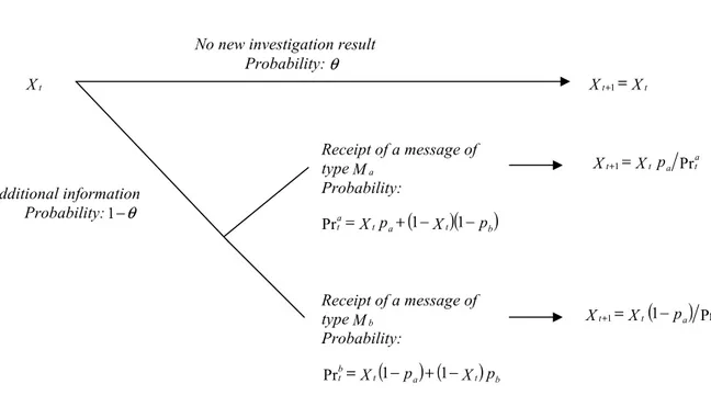
Let Xt (respectively 1 Xt) denote the subjective probability at time t that the true scenario is the optimistic (respectively pessimistic) scenario. In order to make the dynamics of Xt more explicit, we consider that they are two types of informative messages that may be received on one period of time. The first type is a message Ma which is more likely when the correct scenario is the optimistic scenario. Ma is received with probability (conditional on the arrival of an informative message) p_a 1 2 if the correct scenario is the optimistic scenario and with probability (conditional on the arrival of an informative message) 1 p_b 1 2 if the correct scenario is the pessimistic scenario. The second type of message is a message Mb which is more likely when the correct scenario is the pessimistic scenario. Mb is received with probability (conditional on the arrival of an informative message) p_b 12 if the correct scenario is the pessimistic scenario and with probability (conditional on the arrival of an informative message) 1 p_a 12 if the correct scenario is the optimistic scenario. Accordingly, given that an informative message is received, economic agents consider that there is a probability Xtpa Xt pb

a

t 1 1

Pr that it is a message Ma and a probability

p X p Xt a t b b t 1 1

Pr that it is a message Mb. Probabilities pa and pb are objective probabilities known by all economic agents. As a result, economic agents are assumed to revise their beliefs on the correct scenario by applying Bayes’ theorem. This yields the dynamics of beliefs illustrated by Figure 1. A key feature of the stochastic process Xt representing these beliefs is that it admits two absorbing points which are respectively _Xt 0 and _Xt 1_{. This is consistent with the fact that Xt} is a probability and does not take values outside the interval 0,1 when starting from the interior of this interval. It also reflects the fact that when economic agents have no doubts about what is the correct scenario they will never change their beliefs whatever the type and number of new messages received.

Insert Figure 1

2.2Bayesian learning and decision errors: an example

In the context of the use of GMO for agricultural purposes, investigation takes the form of scientific tests to determine whether a GMO plant may disseminate easily or not. The optimistic scenario corresponds to the absence of dissemination. In this case, producers adopting the GMO plant do it in their own interest so that there are exclusively net benefits. The pessimistic scenario corresponds to a significant dissemination of the GMO plant, more specifically dissemination on fields devoted to organic agriculture. As a result products harvested on these fields no longer conform to the rules of organic agriculture and cannot be sold under the organic label, thus implying a loss for organic producers. For the problem to make sense, the loss incurred by organic producers is supposed to exceed the benefit of

farmers adopting the GMO plant so that there is a net loss. Scientific tests may invalidate some factors alleged to induce GMO dissemination. Such a conclusion is logically more likely to occur under the optimistic scenario and is assimilated to a message of type Ma. Conversely, scientific tests may confirm factors alleged to induce GMO dissemination. Such a conclusion is assimilated to message of type Mb because it is more likely to occur under the pessimistic scenario. Probability 1 p_b reflects the risk that no dissemination is proven by scientific tests in spite of its existence, due to measurement errors and/or inappropriate protocols. Probability 1 p_a captures the risk that a conclusion in favour of dissemination is obtained whereas the correct scenario is that without dissemination. Such a risk originates in errors in the protocol or manipulations and is clearly expected to be far lower than the previous risk. These two types of risk are referred to as the risk of first type and the risk of second type in statistics. Table 1 adapted from Dorman (2005) helps illustrating the nature of the risk conditionally on the correct scenario and the decision. It also helps understanding the debate between the partisans of GMOs and their opponents. On the one hand, partisans of GMOs stress the risk of a ban of GMOs whereas they may constitute a major innovation for economic and human progress. What they have in mind is the risk of first type. By sometime disregarding the risk of second type they implicitly reveal that they believe without doubt that the correct scenario is the optimistic scenario (i.e. _X0 1). On the other hand, opponents to GMOs point out the threat of an irreversible dissemination of GMO plants and thus have in mind the risk of second type. They sometime do not mention the risk of banning a harmless and profitable innovation and thus implicitly reveal that they believe without doubt that the correct scenario is the pessimistic scenario (i.e. _X0 0). For this two polar positions, scientific investigation aiming at obtaining additional information is worthless because both

1

Xt and Xt 0 are absorbing points of the stochastic process describing the dynamics of beliefs and thus both extreme partisans and extreme opponents are locked in their initial beliefs. Scientific investigation makes sense only in the presence of some initial doubts. A reasonable position could consist for instance in affecting a same probability (i.e. _X0 12) to each scenario to reflect the absence of a priori about the problem at stake. Beliefs then evolve through time as new information is received and how the risks of first and second types should be balanced is a dynamic matter.

Insert Table 1

What distinguishes our modelling assumptions form the standard model of Arrow and Fisher (1974) and the subsequent works applying the real option theory to the analysis of optimal choice when facing risk and irreversibility is the explicit Bayesian nature of the underlying stochastic process. Indeed, the dynamics of beliefs used in Arrow and Fisher (1974) is obtained as the peculiar case of the stochastic process described in Figure 1

with 0 , p_a 0 and p_b 0. Said less formally, Arrow and Fisher (1974) consider an informative message is received for sure and, moreover, it is not a noisy message. As a result, waiting one period of time enables switching from incomplete to complete information so that the dynamics of the problem is fully handle by a two period model. From a technical point of view, these additional assumptions imply that the stochastic process does not depart from a standard Markovian process. This is less obvious if errors of first type and/or errors of second type are introduced.

3.A BAYSIAN REAL OPTION APPROACH TO THE OPTIMAL DEVELOPMENT DECISION

This section starts with the decision problem of a public authority having to maximise the intertemporal utility of a representative agent. Reference to the agent’s preferences is thus explicit but the problem departs from a standard model of precautionary saving by the discrete nature of the decision (3.1). It is shown that the optimal decision rule may be determined as the optimal exercise rule of a real option problem (3.2). A numerical example is provided to highlight how the perspective of acquiring costly information may drastically reduce the set of state of beliefs for which either definitive abandonment or immediate development is optimal, thus calling for postponement of project and further scientific investigation about its consequences (3.3).

3.1The decision problem

The public nature of the decision to develop or not the innovative project in the canonical problem introduced in the previous section arises from two elements. First, as they generally correspond to previously unobserved phenomena, no mechanism exists to internalise the potential harmful impacts of the development of the innovative project. Second, scientific knowledge is a non rival good the production of which is suboptimal if let to private economic agents. With these two elements in mind, we consider a public authority facing the problem to either abandon the innovative project or develop it immediately or postpone the development while financing scientific investigations about its consequences. There is a representative agent or equivalently numerous identical agents with an additive intertemporal utility where uY ,Q stands for the instantaneous utility function and denotes the utility discount rate. The instantaneous utility function depends on the consumption level Y and on the level Q of environmental quality or health. Consumption amounts to y units in the absence of development and scientific investigation. In case of an immediate development of the project, the consumption level raises to y B~ where B~ is the random additional benefit expressed in terms of consumption units that the project generates for all future dates. In the optimistic scenario, environmental quality (or health) is preserved when the project is developed so that Q remains equal to its initial level q . The instantaneous

utility level is then given by u y B~,q . Conversely, the pessimistic scenario implies that Q falls to q D~ where D~ is the measure of random damages in physical terms and the resulting instantaneous utility level for all future dates is u y B~,q D~ . The exact values of additional consumption and damages are unknown until the project is developed. Risk as regards these values is introduced in order to analyse the impact of risk aversion and link our results to that of Gollier et al. (2000). B~ and D~ have known probability distributions. For the problem to make sense we also assume that u y B~,q D~ u y,q whatever the realisations of B~ and D~. Finally, the consumption level is given by y C as long as postponement of the development and further scientific investigation is decided, which yields the instantaneous utility level u y C,q . The public authority seeks to maximise the intertemporal expected utility of the representative agent. In case of abandonment, the intertemporal utility level is deterministic and defined by

WA 0 ₁ , t t q y u q y u , 1 (1)

In case of an immediate development without damages, the intertemporal expected utility level is given by the same expression with Eu y B~,q in place of u y,q . The corresponding expression in case of damages deserves more attention. Indeed it is not standard to use the expected utility model with a utility function having two random arguments. Therefore, we first express the instantaneous utility level obtained with the pessimistic scenario in terms of the willingness to pay W~ for preserving environmental quality or health. By definition we have u y B~ W~,q u y B~,q D~ so that only the first argument of the instantaneous utility function is random. Accordingly, the intertemporal expected utility level in case of damages is given by the same expression than (1) with

q L y u

E ~, in place of u y,q where L~ W~ B~ stands for random net equivalent losses expressed in consumption units and associated with damages to the environment or health. Note that the second argument in u remains unchanged whatever the situation considered. In order to make notations more concise we thus replace u by v with consumption as the sole argument thereafter. Function v may be interpreted as an indirect utility function. Therefore, the expected intertemporal utility level, conditional on information received so far, when immediate development is decided but just before development reveals whether there are damages or not is defined as

L y v E X B y v E X X W t t t D 1 ~ ₁ 1 ~ ₍₂₎

Postponing the development while financing scientific investigation about its consequences yields the instantaneous utility level v y C u y C,q at the current date plus the expected discounted intertemporal utility level corresponding to the optimal choice between definitive abandonment, postponement with scientific investigation and immediate development at the next date. Therefore, the optimal expected intertemporal utility level at the current date is given by

X W p X W p X W X W C y v W Max X W t D b t a t b t a t a t a t t A t 1 Pr 1 * Pr Pr * Pr 1 * * (3) The expected optimal intertemporal utility level at the next date in case of postponement is defined on the basis of the dynamics of beliefs described in Figure 1. With probability no additional informative message is received in spite of scientific investigation. The optimal intertemporal utility level then remains unchanged. With probability 1 Pra

t it is believed that a message of type Ma will be received and thus that an upward revision to

Pr

1 t a at

t X p

X of the beliefs that the optimistic scenario is the correct one will occur at date 1

t _{. Conversely, it is believed that a message of type M}b will be received with probability

Pr

1 b

t and that a downward revision to Xt 1 Xt 1 pa Prbt of the beliefs that the optimistic scenario is the correct one will occur at date t 1.

Whether postponement has to be preferred to definitive abandonment or immediate development crucially depends on the state of beliefs Xt. If there were non perspectives of acquiring additional information through time (i.e. if 1) it would never be optimal to postpone the decision. Indeed, it would imply to incur the investigation cost without perspectives to change the state of beliefs. This also happens if beliefs are locked to Xt 1 or

0

Xt , even if informative messages are received. According to the discussion made in the previous section about the respective positions of extreme opponents and extreme partisans of the development of innovative projects susceptible to have harmful impacts on the environment and /or health, this explains why both of them reject the idea of further scientific investigations. Whatever the reason, if the perspective of acquiring more information is disregarded, the optimal choice consists in developing immediately the project when

W X

immediate development is preferred if and only if Xt exceeds a threshold value defined as a ratio of variations for the instantaneous utility level:

X X W X WD t A t (4.a) with L y v E B y v E L y v E y v X _{~ ~} ~ (4.b)

If the perspective of acquiring more information is taken into account, a definitive abandonment of the project as soon as _Xt X could reveal to be suboptimal at the next date. It more specifically happens if messages of type Ma (leading to an increase of Xt) are received. Conversely, an immediate development of the project as soon as _Xt X could be regretted if the pessimistic scenario reveals to be the correct one. Indded, waiting just one period of time more could induce the receipt of a message Mb leading to a drop of Xt and thus justifying not to develop the project. Therefore, taking account of the arrival of additional information, it is optimal postponing the decision to abandon or develop the project as long as beliefs stay inside an interval _XA_{, X}D _{where X}

XA is the lower bound behind which definitive abandonment is optimal and XD X is the upper bound above which immediate development is optimal. In mathematical terminology, is the optimal waiting region of the optimal stopping time problem defined by (3). The optimality of this form of waiting region is checked ex post by verifying that the resulting intertemporal utility level W _Xt

* _exceeds

both WA and W _Xt D

for values of Xt in .

3.2The option value of additional information

The optimal thresholds XA _{and X}D _{are find by solving the optimal stopping time} problem (3). For this purpose, note that as long as Xt lies inside the optimal waiting region

the value function _W* _{Xt satisfies the following definition}

X W* t v y C 1 * X W t X X X p X W p X W D A t b t a t b t a t a t a t , 1 Pr 1 Pr Pr Pr 1 * * (6)

This is nothing else than the discrete time version of the Bellman equation characterising option values in continuous time real options problems. Substitution shows that the

homogeneous part of the equation has solutions of the form X X X X K X W t t 1 t t 1 t

* _{, provided is a root of the characteristic equation}

p p p p p p b b a b b a 1 1 1 1 1 (7)

For a strictly positive discount rate the left hand side of equation (7) is a positive, higher than unity, constant. Let h denote the right hand side of equation (7). It is easily checked that h 0 1 and h1 1. Moreover, given that p_a 1 2 and p_b 1 2 some computations

lead to the conclusion that lim h , lim h , h 0 and

0

h with 0,1 . As illustrated by Figure 2, we can conclude that (7) has two roots satisfying 1 1 and 2 0. Then, solutions of the homogeneous part of equation

(6) are linear combinations of the two independent solutions

X X X X X f1 t t 1 t t 1 t 1 and f2 Xt Xt 1 Xt Xt 1 Xt 2. Solutions to the complete equation (6) are obtained by adding the particular solution

C y v

WP 1 (8)

A parallel with (1) shows that this particular solution defines the intertemporal utility level in case of permanent postponement and investigation. Of course, it is expected that postponement will not be permanent and that at some date in the future a sufficient amount of information will be acquired so that it will be optimal to either abandon the project or develop it. This perspective justifies incurring the investigation cost for acquiring more information and generates an option value, expressed in terms of utility, that adds to WP in order to obtain

X

W* t . The expression of this option value OV Xt is given by the general solution to the homogeneous part of equation (6). Therefore

X OV X f K X f K W C y v X W t t t P t 1 1 2 2 * 1 ₍₉₎

Where the two constants K1 and K2 remain to be determined on the basis of the behaviour of

the value function W _Xt

* _{at the boundaries of the waiting region.}

3.3Solution to the optimal stopping problem

By definition, at the lower bound XA _{of the waiting region the public decider is just} indifferent between postponing the development of the innovative project and definitely abandoning it. As a result the following condition holds

W X

W* A A (10.a)

Similarly, at the upper bound XD _{of the waiting region the public decider is just indifferent} between postponing the development of the innovative project and immediately realising it. This yields the second boundary condition

X W X

W* D D D (10.b)

In the terminology of optimal stopping time problems, (10.a) and (10.b) are the “value matching” conditions. Solving simultaneously (10.a) and (10.b) with respect to K1 and K2

generates expressions K1 XA,XD and K2 XA,XD of these two constants as functions of

the two thresholds XA

and XD_{. These two expressions are the only way by which the levels} of XA

and XD _{affect the level of the value function} X

W* t . The other conditions required to obtain XA

and XD _{are the “smooth pasting” conditions}3

0 * X WX A (11.a) and X W X W*X D DX D (11.b)

Where W*X Xt and WDX Xt respectively stand for the first derivative of W* Xt and X

WD t with respect to Xt. It seems that it is not possible to obtain an analytical solution for XA and XD_{. Therefore we turn to a numerical solution to illustrate the optimal decision rule} and visualise the importance of the additional intertemporal expected utility generated by the opportunity to postpone realisation of the project in order to acquire more information. The instantaneous indirect utility function is assumed to take the form v y y and parameters values used for the numerical application are p_a 0.6, p_b 0.9, 0 , .1 0 , .5 0.03,

100

y , B 10, L 25 and C 1. The associated optimal thresholds values are 246074

. 0

XA and XD 0.88062. Figure 3 confirms that W* Xt exceeds W A _and

X WD t for all values of Xt between XA and XD. The threshold to be used in the absence of the

3

See Brekke and Oksendal (1991), Dumas (1991) or Dixit (1993) for technical details on the link between the optimality of the thresholds values and the smooth pasting conditions. Sodal (1998), Dixit et al. (1999) or Shackleton and Sodal (2005) provide an alternative, equivalent but more intuitive for economists, explanation of optimality conditions for basic option problems.

opportunity to acquire new informative messages as time goes is X 0.732969. The optimal waiting region is not centred on this latter value but extends more on its left than on its right. The perspective to acquire additional information thus plays more in favour of a reduction of the range of beliefs that justifies definitive abandonment of the project than in favour of a reduction of the range of beliefs in favour of an immediate realisation of the project. In spite of a wide optimal waiting region, the supplement of intertemporal expected utility generated by the opportunity to postpone the project and pay for additional information remains rather limited. It amounts at most to 1.26% of WA at X X.

Insert Figure 3

4.IMPLICATIONS FOR THE COST BENEFIT ANALYSIS OF INNOVATIVE PROJECTS

When facing projects without macroeconomic incidence, public authorities generally implement a Costs Benefits Analysis. This section examines how to make such a Costs Benefits Analysis consistent with the approach to the precautionary principle developed so far in the article. Rewriting the problem in terms of monetary units requires adding corrections to gross measures of costs and benefits in order to correctly take account of preferences (4.1). The real option model with Bayesian learning presented in the previous section may then be converted from a problem in terms of utility to a problem in terms of monetary units (4.2).

4.1Switching from utility to monetary units

Implementing Cost Benefit Analysis to the problem of developing, abandoning or postponing the innovative project presumes that net benefits and net losses incurred in case of development but also investigation costs associated to postponement are small compared to the initial consumption level y . The indirect utility function may then be replaced by its second order approximation in the neighbourhood of the initial consumption level. In the case of postponement, the instantaneous utility function is thus replaced by

C y v C y v y v C y v ₁₂ 2 ₍₁₂₎

Moreover, utility terms have to be converted in monetary units by dividing by the marginal utility level v y . We then obtain the following decomposition of (12)

m C y v y v C v y v y v v y v C y v p a p 2 2 1 (13)

where vp is the instantaneous utility level in terms of monetary units obtained in case of postponement and investigation whereas va is the instantaneous utility level in terms of monetary units obtained in case of abandonment. Postponing the project to benefit from scientific investigations not only induces the additional investigation cost C compared to abandonment but also an additional monetary value referred to as expression mp. Given that the marginal utility of consumption is positive but decreasing, mp is a cost. Imposing constant marginal utility of consumption is the only way to obtain a value of zero for mp. Therefore, mp is interpreted as the equivalent monetary penalty to be added to the investigation cost C to take account of the decreasing marginal utility of consumption. Substituting L~ to C in (13), taking expectation and noting that the variance of net losses is given by 2 ~2 2

L t L EL

with _L E L~ their expected value, we obtain a somewhat similar decomposition of the monetary equivalent vL of the instantaneous utility level in case of development and net losses L L L L a L t y v y v m y v y v v y v y v v y v L y v E L 2 2 2 1 2 1 ~ (14)

In addition to the monetary penalty mL due to the decreasing marginal utility of consumption, the expected loss _L is also reduced by the Arrow Pratt approximation _L of the risk premium. The fact that both the decreasing marginal utility of consumption and risk aversion are captured by the concavity of the instantaneous utility function implies that mL and L have close expressions. The decomposition is almost identical except the negative sign of the second term of the right hand side in case of development and net benefits:

B B B B a B y v y v m y v y v v y v y v v y v B y v E B 2 2 2 1 2 1 ~ (15) where _B and 2

B respectively denote the expected value and variance of net benefits. Note that whether losses or benefits are considered, taking account of the marginal utility of consumption always yields a penalty.

4.2Precautionary principle in terms of costs and benefits

The next step to switch from the utility maximisation problem to a Cost Benefit Analysis problem consists in rewriting program (3) in terms of variations of the expected intertemporal utility level compared to the level WA obtained with abandonment and dividing

all expressions by the marginal indirect utility v y to convert all terms in monetary units. Using approximations (13) (14) and (15) and proceeding along the same lines than in section 3, the option value is now defined in monetary units by two constants _{K1 K1} v y and

y v K

K 2 2 that solve the following two “value matching” boundary conditions replacing

boundary conditions (10.a) and (10.b)

0 1 2 2 1 1 f X K f X K m C A A p (16.a) X f K X f K m C D D p 1 1 2 2 1 L L L D B B B D m X m X 1 1 1 (16.b)

The optimal thresholds XA

and XD _{of beliefs solve the following “smooth pasting”} conditions that replace boundary conditions (11.a) and (11.b)

0 2 2 1 1 f X K f X K X A A X (17.a) X f K X f K X D D X 2 2 1 1 B mB B L mL L 1 (17.b)

where the subscript X is used to denote the derivative of functions with respect to the state of beliefs.

Finally, boundary conditions (16.a), (16.b), (17.a) and (17.b) are those obtained when directly solving the optimal stopping time problem defined by

t L L L t t B B B t b t a t b t a t a t a t t p t m X m X p X V p X V X V m C Max X V 1 1 1 1 Pr 1 Pr Pr Pr 1 0 (18)

Expression (18) corresponds to (3) expressed in terms of monetary costs and benefits. V _Xt

is the monetary option value of postponing the project to acquire additional information at the cost C _mp, to be thought of as the exercise price of the option. Abandonment yields a monetary value of zero corresponding to the first line in (18). Development of the project generates the flow _{B mB B} of benefits for all future dates if the optimistic scenario is the

true scenario whereas the flow _L m_{L L} of losses is generated if the pessimistic scenario is correct. Both flows are discounted at rate and corrected to take account of decreasing marginal utility of consumption and risk aversion. By this way, preferences and attitude toward risk affect the optimal decision rule. Given the current state of beliefs Xt, development of the project yields the expected discounted monetary value that appears in the third line of (18). According to (18), the project is valued by the expected discounted sum of benefits and losses, respectively weighted by the current beliefs that the correct scenario is the optimistic scenario or the pessimistic one, if and only if immediate development is optimal. This occurs when _{X X}D

t . The project is worthless if the current beliefs in favour of the optimistic scenario fall below the threshold XA_{. Finally, the project is valued at the option} value X f K X f K m C X V t p 1 1 t 2 2 t 1 (19)

for all states of beliefs such that Xt is in the range X X D

A_{, . This value may be used, for} instance, to define the maximal initial investment cost that justifies not abandoning the project. The optimal exercise rule of the real option highlights how to balance costs and benefits in the presence of evolving scientific uncertainty about potential irreversible impacts. Costs and benefits are not only weighted by current beliefs, they also play a key role in defining the optimal thresholds of the state of beliefs above which immediate realisation of the project is optimal and below which definitive abandonment has to be chosen. As regard this second effect, their influence is highly non linear if the perspective of acquiring costly additional information is properly taken into account.

5.CONCLUSION

The canonical model developed in this article is intended to provide a guideline for implementing the precautionary principle in Cost Benefit Analysis. First, it builds on the real option theory but extends it to Bayesian learning processes instead of the standard Markovian processes generally postulated in the literature. This extension makes the real option approach more consistent with the logic of evolving scientific knowledge that is at the core of the precautionary principle and results from a costly search for additional information. Second it conciliates the real approach to precautionary principle and the strand of literature that analyses the precautionary principle by adapting the concept of precautionary saving to environmental preservation. This suggests applying two kinds of correction to flows of costs and benefits. The first correction is intended to take account of the marginal utility of consumption. The second correction follows on from risk aversion and takes the form of a risk premium. Using standard method of resolution of real options models, it is then shown

how corrected costs and benefits influence the choice between abandoning, realising or postponing innovative projects with uncertain but irreversible potential harmful effects.

REFERENCES

Arrow, K. J., Fisher, A. C., 1974. Environmental Preservation, Uncertainty, and Irreversibility, Quarterly Journal of Economics 88, 312-319.

Brekke, K. A., Oksendal, B., 1991. The high Contact Principle as a Sufficiency Condition for Optimal Stopping. In Lund, D., Oksendal, B., (Eds.), Stochastic Models and Option Values. North-Holland, New York.

Brennan, M. J., Schwartz, E. S., 1985. Evaluating Natural Resource Investments. Journal of Business 58, 135-157.

Dixit, A., 1992. Investment and Hysteresis. Journal of Economic Perspectives 6, 107-132.

Dixit, A., 1993. The art of smooth pasting. In Lesourne, J., Sonnenschein, H. (Eds). Fundamentals of pure and applied economics, Vol 55. Harwood Academic Press, Chur Switzerland.

Dixit, A., Pindyck, R. S., 1994. Investment Under Uncertainty. Princeton University Press, Princeton.

Dixit, A., Pindyck, R. S., Sodal, S., 1999. A markup interpretation of optimal investment rules. The Economic Journal, 109, 179-189.

Dorman, P., 2005. Evolving knowledge and the precautionary principle. Ecological Economics, 53, 169-176. Dumas, B., 1991. Super Contact and related Optimality Conditions. Journal of Economic Dynamics and Control

15, 675-685.

Fisher, A. C., 2000. Investment under Uncertainty and Option Value in Environmental Economics. Resource and Energy Economics 22, 197-204.

Fisher A. C., Hanemann, W. M., 1987. Quasi-option Value: Some Misconceptions Dispelled. Journal of Environmental Economics and Management 14, 181-190.

Freixas, X., Laffont, J-J., 1984. On the Irreversibility Effect. In Boyer, M., Kihlstrom, R., (Eds.). Bayesian Models in Economic Theory. Elsevier, Dordrecht.

Gollier, C., Jullien, B., Treich, N., 2000. Scientific progress and Irreversibility: an Economic Interpretation of the Precautionary Principle. Journal of Public Economics 75, 229-253.

Gollier, C., 2001. Should we beware of the Precautionary Principle?. Economic Policy 16, 301-328.

Hanemann, W. M., 1989. Information and the Concept of Option Value. Journal of Environmental Economics and Management 16, 23-37.

Henry, C., 1974. Investment Decisions Under Uncertainty: The Irreversibility Effect. American Economic Review 64, 1006-1012.

Immordino, G., 2003. Looking for a guide to protect the environment : the development of the precautionary principle. Journal of Economic Surveys 17, 629-643.

Kelly D. L., Kolstad, C. D., 1999. Bayesian Learning, Growth and Pollution. Journal of Economic Dynamics and Control 23, 491-518.

Kolstad, C. D., 1996a. Learning and Stock Effects in Environmental Regulation: The Case of Greenhouse Gas Emissions. Journal of Environmental Economics and Management 31, 1-18.

Kolstad, C. D., 1996b. Fundamental Irreversibilities in Stock Externalities. Journal of Public Economics 60, 221-233.

Lund, D., 1991. Financial and Non Financial Option Valuation. In Lund, D., Oksendal, B., (Eds.). Stochastic Models and Option Values. North Holland, New York.

McDonald, R., Siegel, D. R., 1986. The Value of Waiting to Invest. Quarterly Journal of Economics 101, 707-727.

Pindyck, R. S., 1991. Irreversibility, Uncertainty and Investment. Journal of Economic Literature 29, 1110-1152. Pindyck, R. S., 2000. Irreversibilities and the timing of environmental policy. Resource and Energy Economics

Shackleton, M. B., Sodal, S., 2005. Smooth pasting as rate of return equalization. Economics Letters 89, 200-206.

Sodal, S., 1998. A simplified exposition of smooth pasting. Economics Letters 58, 217-223.

Figure 1 Dynamics of beliefs

Additional information Probability:

Xt

No new investigation result Probability: X Xt 1 t 1 Receipt of a message of type Probability: Ma p X p Xt a t b a t 1 1 Pr Receipt of a message of type Probability: Mb p X p Xt a t b b t 1 1 Pr Pr 1 a t a t t X p X Pr 1 1 t a bt t X p X

Figure 2

Solutions to the characteristic equation

h 1 1 2 1 1 0 1

Figure 3

Optimal waiting region and intertemporal expected utility levels as function of the state of beliefs in the numerical example.

0.2

0.4

0.6

0.8

1

X

330

335

340

345

350

355

360

X

X

W

W

X

W X

Table 1

Typology of decision errors

Correct scenario :

H0

Optimistic scenario

H1

Pessimistic scenario

H0 No error Error of type 2

Conclusion :