Évaluation des déterminants de l'aire de répartition des poissons d'eau douce pour éclairer leur écologie et conservation

(1)

THÈSE

En vue de l’obtention du

DOCTORAT DE L’UNIVERSITÉ DE TOULOUSE

Délivré par l'Université Toulouse 3 - Paul Sabatier

Cotutelle internationale : Instituto de Ecología A.C.

Présentée et soutenue par

JUAN CARVAJAL-QUINTERO

Le 9 octobre 2020

Évaluation des déterminants de l'aire de répartition des poissons

d'eau douce pour éclairer leur écologie et conservation

Ecole doctorale : SEVAB - Sciences Ecologiques, Vétérinaires, Agronomiques et Bioingenieries

Spécialité : Ecologie, biodiversité et évolution Unité de recherche :

EDB - Evolution et Diversité Biologique Thèse dirigée par

Thierry OBERDORFF et Fabricio Villalobos Jury

M. David NOGUéS-BRAVO, Rapporteur M. Paulo PETRY, Rapporteur Mme Elizabeth ANDERSON, Examinatrice

M. Sébastien BROSSE, Examinateur M. Pablo TEDESCO, Examinateur M. Fabien LEPRIEUR, Examinateur M. Thierry OBERDORFF, Directeur de thèse M. Fabricio VILLALOBOS, Co-directeur de thèse

(2)

(3)

(4)

(5)

Acknowledgements

First of all, I want to thank my co-directors Pablo, Fabricio, and Thierry for their continuous support during my PhD. Thank you for ALWAYS being willing to solve my questions and offer me a guide in the moments that I was lost in my seas of ideas and data. Thanks to Pablo for the serenity that he always transmitted to me to face the challenges, to Fabricio for his enthusiasm and vibrant energy to explore new ideas, to Thierry for his objectivity in all our discussions.

Thank you very much to David Nogues Bravo, Paulo Petry, Carla Gutierrez, Andres Lira, Elizabeth Anderson, Fabien Leprieur and Sebastien Brosse for being reviewers and/or members of the thesis jury. Your comments will be very important to improve this manuscript and to broaden and strengthen the foundations of the line of research that I am building. Many thanks to Gaël Grenouillet and Alejandro Espinosa, members of my thesis committee, for their advice and opinions during the 8 thesis committees, a great proof of patience!

I am very grateful to the following institutions for their financial and logistical support to carry out my thesis: Consejo Nacional de Ciencia y Tecnología de Mexico (CONACYT), Office français de la biodiversité (OFB), INECOL A.C., Université Paul Sabatier, Laboratoire Évolution et Diversité Biologique, Institut de Recherche pour le Développement (IRD), Society for Conservation Biology (SCB), Labex Tulip, y los proyectos AMAZONFISH y ODYSSEUS (ERANetLAC and BiodivERsA founded projects respectively).

Mil gracias a Ana por su amor, compañía, incondicionalidad y alegría durante este tiempo, sin duda fue un viaje inolvidable.

A mi familia porque a pesar de no entender mi trabajo y el porqué lo estoy haciendo siempre me han apoyado.

A Javier Maldonado Ocampo por haberme transmitido su pasión para estudiar los peces dulceacuícolas, esperó poder transmitir todas tus enseñanzas y el legado que dejaste en mi vida y en mi carrera científica. Eternamente agradecido! Descansa con los peces…

To all the people who have advised and mentored me in my academic training, especially Federico Escobar, Luz Fernanda Jiménez and Stephanie Januchowski

(6)

A Jorge Garcia-Melo por sus fotos, las cuales utilicé en esta tesis y mi defensa. Estas fotos hacen parte del proyecto CaVfish Colombia.

Merci beaucoup à tous les amis de l'EDB (y compris Kathe qui s'est infiltré) de m'avoir accueilli pendant ces trois années, de m'avoir montré l'inconditionnalité de l'amitié française, de m'avoir appris à parler français, et pour faire le silence tous les jours pendant ma sieste :) Gracias a los carnales y carnalas del INECOL y del laboratorio de Macroecología Evolutiva. Los años que pasé en Xalapita la Bella durante mi maestría y principios de mi doctorado siempre estarán en mi mente gracias a ustedes.

À Dominique, Elisabeth, Florence et Claudine pour m'avoir guidé dans la bureaucratie française. Vous faites un travail magnifique.

A Berthita, Ingrid y Mónica por haberme guiado en la burocracia Mexica y por simpre tener una sonrisa de buenos días!

(7)

(8)

(9)

8

CHAPTER 1 ‒ General introduction

Geographic range size

Understanding the geographic distribution of species across space and time is one of the long standing challenges in ecology and evolution. Since the first naturalists of the 18th and 19th centuries, we have documented the enormous variation of species geographic distributions (hereafter geographic range) and have long sought to understand the mechanisms underlying such variation (Brown et al. 1996, Gaston 2003). Despite this, we are still a long way from understanding the principal drivers of range size variation and have a satisfactory explanation about why some species occur in larger area than others (Gaston 2009, Coreau et al. 2010, Sheth et al. 2020). The need to answer these questions has become more urgent in the recent decades as this knowledge is crucial to predict changes in biodiversity patterns in response to global changes, such as, climate change and habitat loss or habitat fragmentation (Brown et al. 1996, Jetz and Rahbek 2002, Gaston 2009, Sandel et al. 2011, Grill et al. 2019).

The species’ geographic range size has been studied across several taxonomic groups and has been related to multiple ecological and evolutionary factors. However, studies on range size have generally analyzed potential driving factors separately or have limited both the number of species and their spatial extent (Brown et al. 1996, Gaston 2003). Indeed, one of the main reasons for the lack of a comprehensive answer to the question of what determines species’ range sizes has been the lack of an holistic view that considers the full extent of species geographic distributions (i.e. extent of occurrence sensu Gaston and Fuller 2009) and the complex way in which multiple driving factors may interact with each other and influence the range size differently among regions and taxonomic groups (Brown et al. 1996, Sexton et al. 2009, Morueta-Holme and Svenning 2018, Sheth et al. 2020).

Some macroecologial studies have made important contributions to the comprehension of the variation on species’ geographic ranges by evaluating quantitatively and statistically, different proprieties of this pattern across the globe (e.g. Li et al. 2016). However, these studies have been only applied to some taxonomic groups, mainly those with more information (e.g. birds and mammals), leaving out many others. Freshwater fishes are one of those groups, still lacking integrative studies describing species distribution patterns. The few studies dealing with the variation of freshwater fishes geographic range size have been species- and location-specific analyses (e.g. Tales et al. 2004, Bertuzzo et al. 2009).

(12)

11 Overcoming these knowledge gaps and applying them to guide conservation strategies for freshwater ecosystems is a critical challenge. Freshwater environments harbor an extraordinary rich and endemic biota, and provide diverse ecosystem goods and services (e.g. providing water quantity and quality as well as food and nutrition for billions of people globally, Costanza et al. 1997, Dudgeon et al. 2006). At the same time, this strong human dependence on freshwater ecosystems’ goods and services drives increased pressures, degrading these ecosystems, modifying species range sizes (Comte et al. 2013, Radinger et al. 2017) and ultimately increasing species’ extinction risk (Vörösmarty et al. 2010, Albert et al. 2020). These human pressures are projected to substantially increase for freshwater ecosystems in the near future, impacting further species’ persistence (Zarfl et al. 2015, Winemiller et al. 2016, Comte and Olden 2017, Albert et al. 2020). Thus, besides understanding the factors and processes explaining species’ geographic range sizes and their changes, it is also important from a conservation perspective to quantify the potential impacts that human-induced changes in range sizes could have on species’ extinction risks, to guide conservation priorities by pointing where actions are needed.

Historical context: From the biodiversity distribution to the species geographic range

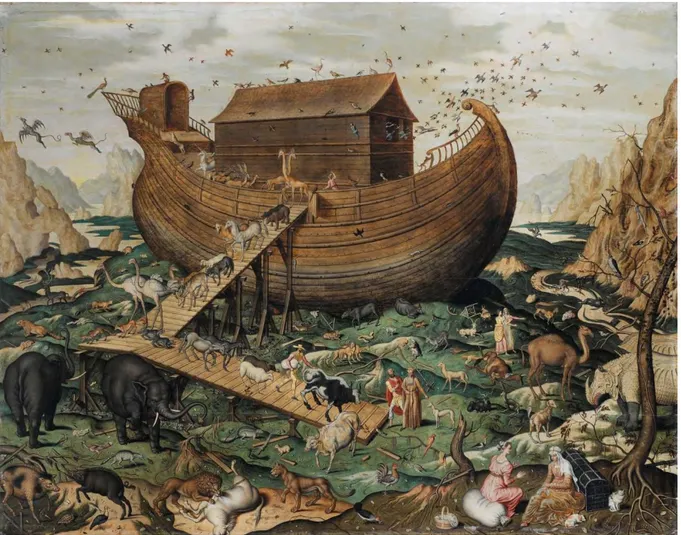
Perhaps, the initial approach to understand the distribution of species was the Noah's Ark, an ancient narrative based on Mesopotamian stories and widely enacted between the 16th_{and 17}th

centuries during the biblical doctrine. Back then, the belief was that after the great flood the animals disembarked from Noah's Ark on Mount Ararat and dispersed around the globe (Fig. 1, Mayr 1982). Thinkers at that time would have predicted the same geographic range size for all the living species. However, in the 18th_{century with the beginning of the age of}

explorations, a vast number of uneven distributed species were described, and it seemed no longer plausible that they all could be aboard an ark (Mayr 1982, Browne 1983). In the mid 18th_{century, Carl Linnaeus, the father of systematics, was the first to think about the}

geography of species distributions alluding a term that later evolved “the regions in which the

plants grow” (Candolle 1820, Nelson 1978). Linnaeus’ interpretation of the distribution of

biodiversity (the mountain explanation) did not rely on dispersal from Noah’s Ark. Instead, he posited that each species was created in a particular climatic belt of a small mountainous island surrounded by a great flood and, as the floodwaters receded, different species dispersed outward from this island to colonize their preferred environments (Browne 1983). The French

(13)

12 naturalist Georges-Louis Buffon challenged Linnaeus’ explanation, recognizing that species were not perfectly suited to an environment; instead, the distribution of species across the globe was the result of the observed shifts in climate (Buffon 1770). Based on this observation, he proposed the Buffon’s law, then known as the “law of the distribution of

forms”, stating that similar environments in isolated regions have distinct species assemblages

with similar attributes (Browne 1983). This law has represented the basis of the first biotic zoning described during the 19th century (see below).

Figure 1. Representation of the Noah’s Ark where animals are descending after the great flood. By Edward Hicks, 1846 Philadelphia Museum of Art. Image obtained from Wikimedia Commons.

In the late 18th_{century, Carl L. Willdenow and Eberhard A. von Zimmermann, two}

German geographers who shared a similar view as Buffon, brought a geological perspective to explain the distribution of species. Based on the observation that different regions and continents shared common species, they proposed that the current distributions of species were the results of historical connections and dispersion processes (Mayr 1982). They also recognized early patterns in the spatial variation of species distribution by describing the

(14)

13 restricted range of plants in mountain regions (Morrone 2009). Willdenow transmitted his passion for plants and mountains to his pupil, Alexander von Humboldt (Hiepko 2006), who in the early 19th century, attempted to get a full picture of the phenomenon gathering empirical evidence to directly relate changes in species distribution with different environmental parameters. Through this evidence, Humboldt set up hypotheses on which factors might influence the physiology of plants and in turn their distribution (Morueta-Holme and Svenning 2018). Perhaps, the strongest relation that he inferred was that the physiological requirements of plants to ambient energy restricted their survival and distribution, which could be clearly seen while ascending a mountain (Fig. 2, Humboldt and Bonpland 1805, reviewed in Morueta-Holme and Svenning 2018). Humboldt also noted the effect of temperature seasonality on species ranges. He attributed the observation that many temperate plants spread from lowlands to high elevations to the fact that species in these regions were exposed to the same low temperatures in winter and at high elevations, and thus, that they have adapted to a wider range of temperatures. Conversely, the stable intra-annual temperature in the tropical regions resulted in clearer vegetation bands towards highlands (Humboldt and Bonpland 1805) (The same observation that lead Janzen to later develop the classic hypothesis “Mountain passes are higher in the Tropics”; Janzen 1967).

(15)

14

Figure 2. Scientific illustrations by Alexander von Humboldt. His famous illustration of Chimborazo volcano in Ecuador shows plant species living at different elevations (Public domain / Wikimedia Commons).

The aforementioned biogeographers were very influential in the study of the distribution of species, identifying biotic zones and how environmental factors determined them. But, the first person that conceived the idea of species geographic range was Augustin de Candolle which described “les habitations” (dwellings), as “the country wherein the plant is native”, and “les stations” (the stations) as “the special nature of the locality in which each species

customarily grows” (Candolle 1820: 383). Another important contribution of de Candolle was

the hierarchical notion distinguishing between the factors that determined the distribution of species on a regional scale (temperature, light and the biology of the organisms) and those that influence global-scale patterns (historical factors that restrict the distribution of species into the provinces) (Lieberman 2012).

During the second half of the 19th_{century, the fields of geology and paleontology added}

an evolutionary view to the distribution of species. At this time, geologists and paleontologists strongly questioned the view that climate alone could explain the distribution of species across the globe, and were looking for reasons why certain species were found in particular areas. Charles Lyell was the first to establish a relationship between the current distribution of species and their distribution in the fossil record. He proposed a deep-time dynamic where the geographic ranges of animals and plants contracted and expanded according to geologically mediated changes (Browne 1983). Charles Darwin, a profound admirer of Lyell, integrated this deep-time dynamic with the thesis that geological changes left descendants with modifications. This allowed Darwin to explain why species distributed in a certain region were more related among them than species found in other distant regions (“On this principle of inheritance with modification, we can understand how it is that sections

of genera, whole genera, and even families are confined to the same areas, as is so commonly and notoriously the case”, Darwin 1859: 350-351). Alfred Russel Wallace extended Darwin’s

vision proposing a global pattern of species distribution, where higher taxonomic hierarchies such asclasses and orders, were generally spread over the whole Earth, whereas more derived ones such as families and genera were confined to more restricted parts of the globe. Overall, the first evolutionary approach of the geographical distribution of species identified that “the

(16)

15 natural sequence of the species by affinity is also geographical” (Brooks 1984: 73). In other

words, that the relationships between species across the tree of life is spatially structured.

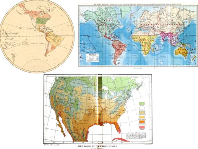
Figure 3. Evolution in the delimitation of geographical-biotic units during the 19th century. Early biotic zones (top) had coarse resolution and strong limits demarcated almost by latitudinal lines whereas Life zones theory (down) integrated climate and topography allowing to reduce resolution and define flexible limits. Top left, first atlas of the geography of plants in the New World, largely based by Humboldt’s collections. By Joakim F. Schouw in 1822 (from Morueta-Holme & Svenning 2018). Top right, bioegraphic regions proposed y Alfred R. Wallace in his book The geographical Distribution of Animals (Public domain / Wikimedia Commons). Down, life zones of the United States proposed by Clinton Hart Merriam (Public domain / Wikimedia Commons).

In the late 19th_{century, an integrated view in the study of natural and social phenomena}

began to permeate the biological sciences (Chamberlin 1965) advocating a more comprehensive view of species geographic distributions, where multiple factors interacted as drivers. Following Chamberlin, Clinton Hart Merriam proposed the “life zones” theory where he stated that climate interacted with topography forming circumpolar belts that aggregated

(17)

16 species in climatic zones (Merriam 1894). The interest of this theory was a finer-resolution view of biotic zoning where borders were adjusted to environmental conditions instead of latitudinal lines (Fig 3). The “life zones” theory was widely accepted in its beginnings, however, in the early 20th century, the supporters of the emerging field of ecology considered that “distribution cannot be explained by the mere mapping of the extent either of

hypothetical faunal divisions” (Ruthven 1920: 248). Ecologists proposed that combining the

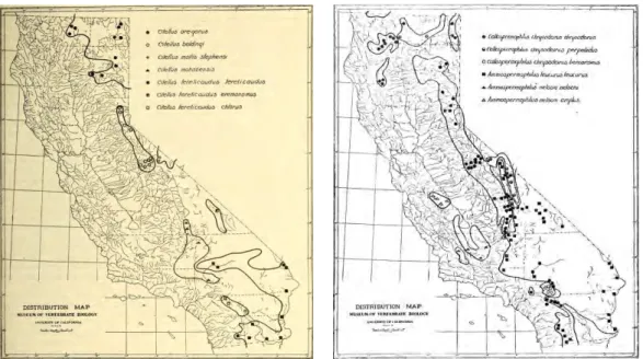
results of experiments altering the intensities of environmental factors along with the study of habitat preferences across the ranges of species was the correct way to identify the determinants of species distribution (Ruthven 1920, Moore 1920). This resulted in the construction of the first regional maps of species’ ranges based on wide sampling records (Fig. 4) and the nomination of different ecological factors as drivers of the species distribution (e.g. Grinnell 1914, 1917, Talbot 1934, Dennis 1938). Besides the contributions made by the field of ecology during the early 20th_{regarding the spatial and environmental component of}

species’ ranges, a temporal dimension was also proposed at that time by John Willis. stated the (Willis 1922). He proposed a positive age-area relationship about the dynamics of species geographic ranges where, in areas with no well-marked barriers, the oldest species would have the broadest geographic ranges.

Figure 4. First regional-distribution maps of ground squirrels species elaborated by Joseph Grinnell (1910, Public domain / Wikimedia Commons).

During the second half of the 20th century, the study of species geographic distributions underwent a pivotal moment and species ranges began to be studied as basic geographic units

(18)

17 (Brown et al. 1996, Jenkins and Ricklefs 2011), transcending the delimitation of biogeographic regions as the only way to explain species distributions and establishing the concept of species range that we currently apply and study (i.e. the area across which a species occurs, Sheth et al. 2020). The first step to consolidate this single-species view of species distribution was the launch of multiple biological surveys (e.g. North American Breeding Bird Survey) and the compilation of maps of geographic ranges for thousands of species that allowed gathering different types of information on the distribution of species (e.g. Hall and Kelson 1959). Then, Eduardo Rapoport used this information to pose the initial guidelines to quantify and analyze different aspects of the species geographic ranges in his seminal book ‘Areografía’ (Rapoport 1975), clearly differentiating between biogeography (“the delimitation of faunistic or floristic sets and in the origin of their different elements”, Rapoport 1975: 21), areography (“the attention on the form and size of the geographical

ranges of species and other taxa”, Rapoport 1975: 21), and ecogeography (“the study of the spatial distribution of taxa, but at a geographic level”, Rapoport 1975: 22). This promoted the

description of early spatial patterns of geographic ranges such as the one showing that small-ranged species are much more common than large-small-ranged ones and that species are not evenly spread through all the potential range (Rapoport 1975, Anderson 1977). Then, these geographic range patterns were rapidly associated with diverse hypotheses: habitat availability (Cody et al. 1975, Anderson and Koopman 1981), density dependent factors (Rosenzweig 1978), abundance (Bock and Ricklefs 1983, Brown 1984), life history (Reaka 1980), and body size (Reaka 1980, Gaston and Lawton 1988).

At the end of the 20th century, the computers-related technology developments facilitated the compilation and digitalization of the first large databases of species ranges, and allowed faster quantification and analysis of distributional patterns. Thus, the study of geographic range size at large spatial scales rapidly received considerable attention (Gaston 1990, 1996, Brown et al. 1996), and the first global patterns were described. One of these patterns is the Rapoport’s rule that describe how species latitudinal range decreased toward the Tropics (Stevens 1989). Other relevant contributions were the macroecological relationships between the geographic range and the body size and abundances of species, documented by James Brown and Brian Maurer (1987, 1989). Through these relationships, Brown and Maurer offered insights into the empirical patterns and causal mechanisms that characterize the distribution of food and space across species (Brown and Maurer 1987, 1989). Today, in the 21th century, these patterns set the basis of macroecological theory

(19)

18 (Keith et al. 2012, Brown 2019) where species geographic range size has been related with a long list of driving factors (Morueta-Holme and Svenning 2018, Sheth et al. 2020). Currently, the study of species geographic range sizes keeps growing, being at the interface of different knowledge fields such as ecology, evolution, biogeography and conservation (Li et al. 2016, McGill 2019, Newsome et al. 2020, Sheth et al. 2020).

Determinants of species geographic range size: going from potential drivers to quantification of interacting forces.

Since the time of Linnaeus, we have identified several extrinsic and intrinsic drivers that shape the variation of species’ geographic range sizes at both ecological (contemporary) and evolutionary (historical) scales (Sheth et al. 2020). Extrinsic drivers are external environmental conditions such as climate and dispersal barriers that directly affect the physiological requirements and morphological variation of species, ultimately determining the presence and accessibility of suitable habitats across the geographical space. Climate stability has been frequently seen as one of the main extrinsic drivers of species geographic range size (Stevens 1989, Morueta‐Holme et al. 2013, Li et al. 2016). At an ecological scale, climate is proposed to select against small range sizes via intra-annual variability (Stevens 1989, Morueta‐Holme et al. 2013, Li et al. 2016). Habitat availability is another prevalent driving factor, small range sizes having been associated with discontinuous areas and habitat fragments (Hawkins and Diniz‐Filho 2006, Morueta‐Holme et al. 2013), or poor habitats representativeness compared to their surroundings (Ohlemüller Ralf et al. 2008). Conversely, widespread habitats can harbor relatively more large-ranged species due to a larger potential for range expansion (Hawkins and Diniz‐Filho 2006, Ohlemüller Ralf et al. 2008). For terrestrial organisms, topographic heterogeneity is also an established driver acting negatively on species geographic range (Hawkins 2006, Li et al 2016), e.g. mountain regions acting as dispersal barriers that constrain dispersal movements through steep-climate gradients and rapid changes of habitats (Brown et al. 1996, Hawkins and Diniz‐Filho 2006, Morueta‐Holme et al. 2013).

Intrinsic drivers of geographic ranges are features of species that condition their response to external drivers (i.e. extrinsic factors) determining their ability to colonize new habitats. Niche breadth (Brown 1984, Slatyer et al. 2013) and dispersal capacity (Glazier and Eckert 2002, Laube et al. 2013) have been proposed as the main intrinsic drivers of species geographic range. Generalist species that can maintain stable or high population densities

(20)

19 across a broad range of environments or resources should become more widespread than specialized species with narrow niches (Brown 1984, Slatyer et al. 2013). Similarly, species with higher locomotion capacities should disperse across longer distances, promoting colonization and achieving larger range sizes (Glazier and Eckert 2002, Laube et al. 2013), whereas, low dispersal ability can lead to population differentiation promoting allopatric speciation into small-ranged species (Gutiérrez and Menéndez 1997). Other species traits related to dispersal capacity have been also associated with geographic range size. For example, when migratory behavior has a low fitness cost, dispersion is expected to be positively related to range size as migratory movements increase the probability of colonizing new areas (Hanski et al. 1993, Polechová 2018). Additionally, the commonly observed macroecological relationship between body size and range size shows an overall positive trend where small-bodied species can have a variety of range sizes, but larger-bodied species are increasingly constrained to larger ranges (Brown and Maurer 1987, 1989; this relationship is explained more in detail below in the section Range - body size relationship, and its

conservation implications of this chapter).

The above drivers explain the ecological reasons for the geographical variation of species range sizes. However, historical factors associated with species’ evolutionary history and/or climatic and geological history of the environment can also influence the size of the area where a species currently occurs. For example, in temperate regions, cyclical variations in the shape of Earth’s orbit induced climatic variability occurring at an evolutionary time scale (104_–106_{year). These variations created long-term climatically unstable conditions that}

may have selected in favor of large range species by lowering the proportion of small-ranged species (Dynesius and Jansson 2000, Jansson 2003, Sandel et al. 2011). The loss of historical barriers can also drive changes in species geographic range size, the connection of previously isolated areas favouring exchanges of biotas that allows the colonization of newly suitable areas and the subsequent expansion of species ranges (e.g. The Great American Biotic Interchange, Vermeij 1991). Conversely, the emergence of geological barriers fragments species ranges into isolated populations promoting speciation events that result in areas with high endemism and composed of species with small range sizes (e.g. the Andes uplift, Hoorn et al. 2010). Regarding time elapsed throughout species’ evolutionary history, the original proposal of the age – area relationship stated that the geographic range of a species continues to expand throughout its life (Willis 1922). However, the fossil record shows a non-linear relation where newly formed species tend to expand their ranges and then undergo a gradual

(21)

20 decline until extinction (Foote et al. 2007, Liow et al. 2010). Average range sizes within clades may also decline with speciation events (Jablonski and Roy 2003, Pigot et al. 2010), as the available space is divided by functionally similar species, leading to a negative relationship between the geographic range size of a species and the diversification rate of the corresponding clade.

Despite the progress already made in identifying several drivers of species’ geographic range sizes, the need to go beyond a long list of factors and to develop a more holistic view of species ranges that allows us to predict how biodiversity patterns will change due to global environmental change is still necessary (Morueta-Holme and Svenning 2018, Sheth et al. 2020). The new models of species geographic range size must consider the interactions among driving factors (Sheth et al. 2020) that directly and indirectly influence its variation while considering the factors’ effects across scales (Levin 1992, McGill 2010), regions (Morueta‐Holme et al. 2013), species traits (e.g. body size, Brown and Maurer 1987), and taxonomic groups (Li et al. 2016) (Fig. 5). This will allow us to have a comprehensive explanation of the distribution of species in specific places and times, but also to dispose of predictive, prescriptive, and scalable models (Hampton et al. 2013).

(22)

21

Figure 5. How driving factors operate? Factors that drive species’ geographic range size can interact (upper right) and influence geographic ranges at different dimensions scales (left). The relative importance of each driver at each scale (represented with gradient colors with respect to each axis; left) varies among them. At the same time, the importance of each driver can vary across each scale (lower right).

This aspiration for a bigger picture of species geographic ranges builds on recent informatics developments and remote sensing technologies that have brought advances in methods and data availability. Large repositories of ecological and environmental data are becoming increasingly accessible (Hampton et al. 2013, Linke et al. 2019, Wüest et al. 2020), and the expansion of computational capabilities has allowed us to better translate our knowledge into empirical and theoretical models with greater inferential strength and causality (Hampton et al. 2013, Connolly et al. 2017). Today, the so-called biodiversity informatics provides us with the opportunity to test hypotheses at unprecedented spatial and temporal scales and integrate disciplines that typically focus on different levels of biological organization, such as phylogenetics, population dynamics, community ecology and macroecology (McGaughran 2015, La Salle et al. 2016, Benedetti‐Cecchi et al. 2018).

Despite being promising, biodiversity informatics is also challenging (Michener and Jones 2012, Hampton et al. 2013, Farley et al. 2018). The enormous amount of information already collected is heterogeneous and spread in different databases or reside on papers or other media from both academic and gray literature, impeding its direct treatment and analysis (Edwards et al. 2000, Farley et al. 2018). Thus, some of the academic and certainly most of the “grey” biodiversity information is often not used for policy or management decisions, nor for scientific research (Edwards et al. 2000). The diversity and scatter of these data lies in the variety of ways in which studies are carried out resulting in large numbers of small and idiosyncratic data sets that accumulate relevant biological, ecological and environmental data collected from thousands of scientists (Michener and Jones 2012). Besides, language barriers and cultural differences across disciplines, institutions and countries hinder the data-sharing (Hampton et al. 2013). Integrating and analyzing massive amounts of heterogeneous data must be carefully planned, and this point is central in contemporary ecological and biogeography sciences (Hampton et al. 2013, La Salle et al. 2016, Wüest et al. 2020).

Thus, through initiatives of developing new databases that make available the massive amount of inconspicuous and disconnected ecological data and the developing of models that

(23)

22 convert these emerging databases into comprehensive and synthetic results, we will be able to have a more holistic vision of species’ geographic ranges to better understand the nature and pace of ecological and environmental changes (Michener and Jones 2012).

Geographic range size of freshwater fishes

One of the most important challenges to achieve a unified view of biodiversity distribution is to contrast the proposed hypotheses and explore new ones across all the tree of life (Shade et al. 2018). However, in the case of geographic range size variation and its drivers, most research has focused on terrestrial environments, mainly for large terrestrial vertebrates (Brown et al. 1996, Sheth et al. 2020), skewing our understanding of species distribution toward a reduced group of charismatic species. Studies about this topic on freshwater fishes are scarce and restricted to specific clades and regions, (e.g. Hugueny 1990, Pyron 1999, Rosenfield 2002, Tales et al. 2004, Blanchet et al. 2013). These studies have identified as intrinsic drivers of range size, factors related to locomotion capacity, energetic requirements and the ability of species to occupy different habitats. For example, fish species presenting migratory behavior, high swimming capacity and small eggs have larger home ranges and a higher probability that offspring disperse and recruit successfully to new suitable habitats, resulting in larger range sizes (Blanchet et al. 2013, Giam and Olden 2018). Likewise terrestrial vertebrates, generalist fish species with larger bodies and presenting high local abundances tend to have larger geographic ranges (Pyron 1999, Tales et al. 2004, Giam and Olden 2018).

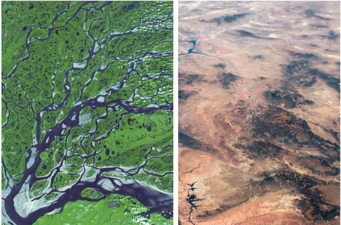
Among extrinsic factors, river topology has been associated with the variation in the range size of freshwater fishes. Bertuzzo et al. (2009) found that fish species with small ranges can be distributed along all the Mississippi-Missouri river basin, whereas, large-ranged species tend to be restricted to the lowland waters. They attributed this pattern to the network structure of rivers (Fig 6) that increasingly constraint the dispersal movements of freshwater organisms toward the headwaters. Similarly, Carvajal-Quintero et al. (2015) found a negative relationship between the species’ regional range size and elevation in Tropical rivers.

River architecture not only restricts dispersion within drainage basins but also among basins, hence freshwater fishes range size may have conserved the signal of historical-geographical patterns (Smith 1981, Hocutt and Wiley 1986). For example, historical connections between rivers (i.e. paleo-connected river drainages) during the last glacial

(24)

23 maximum favored inter-basins colonization (Voris 2000, Dias et al. 2014b) which could have further favored the expansion of geographic ranges of species that inhabited ‘paleo-connected’ basins. Besides, it has been hypothesized that wide river channels and lakes in North America have served as refuges for freshwater fish from adverse environmental changes during glacial periods and allowed them to recolonize northward as glacial sheets retreated (Griffiths 2010, Blanchet et al. 2013), making fish species using large rivers and lacustrine habitats to have larger range sizes than species that do not use these habitats (Giam and Olden 2018).

Figure 6. Topologies of contrasting freshwater (left) and terrestrial environments (right). The branching-network and isolated structure makes freshwater environments more fragmented than terrestrial ones. Images obtained from the NASA earth observatory (https://earthobservatory.nasa.gov/images).

Overall, because freshwater fishes have current and historical dispersal limitations not found among terrestrial taxa, we may expect fish species to display patterns of geographical ranges that differ from birds and mammals, supporting a growing body of literature that suggests that theories developed in open landscapes, such as terrestrial landscapes, may be

(25)

24 inadequate to predict the properties of complex branching ecosystems, such as river networks (Campbell-Grant et al. 2010, Rinaldo et al. 2014).

Geographic range size in conservation

Beyond its theoretical relevance, studying species geographic ranges is also critical for advancing fundamental knowledge in conservation practice and action (Mace et al. 2008, 2010, Lee and Jetz 2011). By identifying the drivers and processes acting on species’ geographic range size we can make projections on the way global change will impact these ranges (e.g. Powers and Jetz 2019), allowing us to develop and prioritize conservation actions for the most affected species. Geographic range size can also be used as a surrogate for identifying species with rapid population decline (Mace et al. 2008), and constantly emerges as a key correlate of extinction risk across animals and plants (Lee and Jetz 2011, Böhm et al. 2016, Chichorro et al. 2019). Additionally, by reflecting the vulnerability of restricted-ranged species, species’ geographic range size analyses play a key role in categorizing species according to their likelihood of extinction (including listing on the IUCN Red List of threatened species) and thus contribute importantly to indices of global trends in threat status and to the prioritization of species for conservation (Gaston and Blackburn 1996a, IUCN 2001, Mace et al. 2008). Indeed, almost 50% of overall threatened species are actually listed as threatened on the basis of the geographic range size criterion alone, and in less known groups, such as amphibians, this could go up to 75% (Gaston and Fuller 2009).

However, the variation of geographic range size by itself does not provide a mechanistic explanation for extinction risk. For example, a small range size alone or a range contraction would fail to detect if population processes needed for the species’ persistence are fulfilled (Mace et al. 2008). Therefore, it is not enough to know that species with small geographic ranges tend to be at greater risk; rather, we need to know how range size interacts with other ecological traits to make certain species more vulnerable than others (Davidson et al. 2009). Thus, by understanding how different key ecological drivers interact, we may be able to identify the species at greatest risk and to understand what makes them vulnerable (Davidson et al. 2009, Ripple et al. 2017).

(26)

25

Range - body size relationship, and its implications for conservation

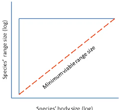
One of the most important patterns accounting for the variation in the size of species’ geographic ranges is the range – body size relationship (Brown 1995, Gaston and Blackburn 2008). This relationship was proposed as a mechanistic explanation on how physical space and resources are allocated among species (Brown and Maurer 1987, 1989), and currently represents the basis of the seminal macroecological theory (Brown 2019). The range-body size relationship is determined by different ecological and evolutionary constraints that restrict the traits space to a triangular envelope through differential colonization, speciation and extinction processes (Fig. 7, Brown and Maurer 1987, 1989). The upper-horizontal bound of the triangle is settled by the maximum geographic area that species can potentially occupy (geographic constraint), the left-vertical bound corresponds to the minimum body size that a species of a given taxon can reach (physiological constraint), and the lower-diagonal bound represents the minimum viable geographic range size needed for species to achieve long-term persistence given their body sizes (Fig. 7, Brown and Maurer 1987, 1989, Gaston and Blackburn 1996).

Figure 7. Empirical model describing the geographic range size–body mass relationship proposed by Brown and Maurer (1987, 1989).

(27)

26 Two main hypotheses have arisen to explain the lower-diagonal bound of the range-body size relationship. First, large-bodied species tend to disperse more quickly and efficiently than smaller species filling a bigger portion of their potential distributional range (Gaston 1994a, Gaston and Blackburn 1996a). Second, large species have higher energetic demands than small species, hence large-bodied species occupy larger home ranges to attain enough resources to support viable population size to be able to persist (Brown and Maurer 1987, Swihart et al. 1988). Thus, small species can have a variety of geographic range sizes while species with larger body size are restricted to larger ranges (Gaston and Blackburn 1996a).

From a conservation perspective, the lower-diagonal bound of the range – body size relationship is the most important feature and has been proposed as a probabilistic vulnerability limit whereby any species that is near or beyond this limit is prone to extinction or has a low probability of persistence through time (Brown and Maurer 1987, 1989, Gaston and Blackburn 1996a). Different studies have shown that the distance of species with respect to the lower limit is a reliable and useful predictor of extinction risk (Rosenfield 2002, Diniz-Filho et al. 2005, Le Feuvre et al. 2016, Newsome et al. 2020) and have promoted its use for tracking trajectories of species towards or away from an extinction threshold and to evaluate how different human stressors may affect species vulnerability (Le Feuvre et al. 2016, Newsome et al. 2020).

Despite its applied importance, no test has been done yet to link explicitly this empirical boundary to species’ lower probability of persistence. Providing empirical evidence that directly links this lower limit to a lower probability of species’ persistence or to the minimum viable geographic range size would be a meaningful advance in our comprehension about geographic ranges and vulnerability of species.

Current conservation status of freshwater fishes

Freshwater ecosystems are essential sources of environmental health, economic wealth and human well-being. Freshwaters maintain hydro-climatic regimes in our planet, have provided us food and water for domestic use and agriculture for millennia, sustained transportation corridors, supported recreation, and more recently, enabled power generation and industrial production (Costanza et al. 1997, Dudgeon et al. 2006, McIntyre et al. 2016). At the same time freshwaters harbor an extraordinary diversity of life. Covering about 2% of Earth’s

(28)

27 surface they host approximately one-third of all vertebrate species and 10% of all known species (Strayer and Dudgeon 2010, Reid et al. 2019). Besides, levels of endemism among freshwater species are remarkably high (Dudgeon et al. 2006, Tedesco et al. 2012, Reid et al. 2019). The insular and fragmented nature of freshwater habitats restricts species’ distribution resulting in over half of the freshwater fishes confined to a single ecoregion (Abell et al. 2008).

Despite supporting human well-being and an extremely high biodiversity, the management of freshwater ecosystems worldwide most often focuses on macroeconomic profits and human water security rather than on the benefits provided by the ecosystem integrity (Vörösmarty et al. 2018). Consequently, we are living a freshwater ecosystems crisis (Harrison et al. 2018, Albert et al. 2020) where the current rates of wetlands loss are three times as high as forest loss (Gardner and Finlayson 2018), where populations of freshwater species have declined by an average of 83% since 1970 (more than twice the rate of land or ocean vertebrates, Grooten and Almond 2018), and where extinction rates are exceptionally high (e.g. freshwater fish extinction rates have been estimated to be more than 100 times their natural rates in Europe and United States, Dias et al. 2017).

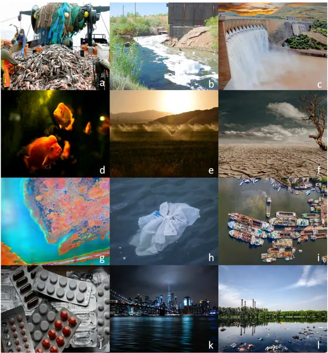
The causes of this biodiversity crisis are widely recognized. Habitat degradation by land use, habitat fragmentation, chemical and organic pollutions, flow modification, overfishing and climate change are the leading causes (Dudgeon et al. 2006, Grooten and Almond 2018, Reid et al. 2019, Albert et al. 2020) (Fig.8). Surface waters receive pollution from commercial activities (e.g. mining, agriculture, oil) and urban settlements, impairing freshwater biodiversity through toxicity or indirect impacts on habitats (Cope 1966). Due to the changes in the use and production of chemicals in the last decades, toxic pollutants are changing and their effects on aquatic populations and communities are largely unknown (Reid et al. 2019). Dams, weirs and levees fragment longitudinal (upstream-downstream) connectivity of rivers and, through flow alterations, also affect lateral (river to floodplain), vertical (surface to groundwater) and temporal (season to season) connectivity, disrupting important processes that support freshwater biodiversity (Albert et al. 2020, Tickner et al. 2020). Today, about 2.8 million of major dams (i.e. dams with reservoir areas >103_m2_{) fragment two-thirds of the}

world’s long rivers (Grill et al. 2019) and dams continue to be built across the globe. Three thousand seven hundred major hydropower dams are currently either planned or under construction (Zarfl et al. 2015), and the increased political and economic support for the widespread development of small hydropower plants (SHP) has resulted in approximately

(29)

28 83,000 SHP operating or under construction (Couto and Olden 2018). Despite the impacts of SHPs are largely unknown, 11,000 new projects already appear in national plans, and if all potential generation capacity were developed, the number of SHP would triple (Couto and Olden 2018).

Figure 8. Major and emerging drivers of freshwater biodiversity loss based on Dudgeon et al. (2006), Reid et al. (2019) and Albert et al. (2020). a) overfishing, b) water pollution, c) dams, d) species introduction, e) land change and water withdrawal, f) climate change, g) algal blooms, h) plastic pollution, i) noise pollution , j) emerging contaminants, k) light pollution, l) declining calcium (eutrophication). There are more threats than those mentioned in this figure,

(30)

29 for more information check original sources. Images obtained from Wikimedia Commons,

Unsplah, and Pexels.

Climate change alters hydroclimates as well as several ecological processes that underlie freshwater ecosystem functioning at different levels of biological organization (Scheffers et al. 2016). Overfishing, that includes both targeted species harvesting and mortalities through bycatch, has persisted during the last decades driving the decline of biodiversity (Allan et al. 2005). For example, overharvesting remains the key threat for the decrease of freshwater-megafauna populations (i.e. animals that reach a body mass of 30 kilograms), that have declined by 88% on average during the last decades, reaching the highest declines in the Indomalaya and Palearctic realms (−99% and −97%, respectively; He et al. 2019). Also, the introduction of invasive species has caused multiple impacts that range from behavioral shifts of native species to complete restructuring of food webs and extirpation of entire faunas (Gallardo et al. 2016).

There is long-standing recognition that environmental stressors can interact affecting freshwater ecosystems through multiple pathways (Ormerod et al. 2010, Vörösmarty et al. 2010, Craig et al. 2017). Thus, emerging and persistent threats can have potential additive effects that might cause multiple ecological alterations, worsening the prognosis for freshwater biodiversity (Reid et al. 2019).

Although for more than two decades scientists have warned about the global biodiversity crisis in freshwater ecosystems, and the low priority given to these ecosystems for global conservation-oriented actions (Brautigam 1999, Dudgeon et al. 2006, Harrison et al. 2018, Albert et al. 2020), freshwater populations continue to decrease rapidly (Grooten and Almond 2018, He et al. 2019) and the actions to safeguard freshwater biodiversity are still “grossly inadequate” (Harrison et al. 2018). This has arisen new emergency recovery plans and recommended actions to promote the restoration of freshwater biodiversity (e.g. Reid et al. 2019, Albert et al. 2020, Tickner et al. 2020).

(31)

30

Thesis

Objective of the thesis

This PhD thesis focuses on identifying the main drivers of geographic range size variation of freshwater fishes at global and biogeographic scales, as well as on understanding the processes that underlie the lower vulnerability limit settled by the range – body size relationship. Results were further applied to the specific case of habitat fragmentation by dams in the Magdalena River Basin (Colombia).

Thesis structure

This thesis is composed of six chapters that address the following topics:

The first chapter consisted in the previous introduction section, where we presented a general context for the species’ geographic range and the range – body size relationship doing a special focus on freshwater fishes, and the importance of these two concepts in conservation science.

The second chapter presents an analysis of global patterns of geographic range size variation of freshwater fishes where we identified the main ecological and historical drivers of fish species’ range sizes at a global scale and tested their consistency across the biogeographic realms. We found that the variation of geographic range size in freshwater fishes is determined by the complex interaction of multiple variables that influence directly and indirectly the geographic range size, and within this complex system the drainage position network and the historical connections among basins account for most of the variation (about 90%). These highlight the importance of current and historical hydrological connectivity in the variation of the geographic range size of freshwater fishes.

In the third chapter, we show an analysis where we assess the lower limit of the geographic range – body size relationship as boundary of lower probability of species’ persistence. For this, we reconstructed the range – body size relationship at a global and biographic realm scales and tested if the lower limit matched with the minimum viable range size represented by the spatial scale of synchrony. We found that the two limits matched at both spatial scales, providing empirical evidence that support the lower limit of the range – body size relationship as a species’ vulnerability limit.

(32)

31 In the fourth chapter, we use the lower limit of the species range – body size relationship to quantify the effect of fragmentation caused by the hydropower development on geographic range and vulnerability of the freshwater fish fauna of the Magdalena drainage basin (Colombia). We also identified the ecological and human-dependency traits of species related to a higher probability of extinction, both intrinsically and because of hydropower development. We found that both existing and planned dams fragment most fish species ranges, and splits species ranges into more vulnerable populations. Importantly, we found that migratory species, and those that support fisheries, are most affected by fragmentation.

The fifth chapter consists of a global database that contains raw data of time series on fish species identities and abundances in different assemblages. This database gathers 11,441 time-series of riverine fish communities, distributed in 11,125 unique sampling locations distributed, and span 21 countries, 5 biogeographic realms, and 402 hydrographic basins worldwide. These data offer the possibility to identify ecological processes underlying species’ geographic range stability as well as to calculate temporal changes in fish diversity at different spatial scales facilitating quantitative analyses of temporal patterns of biodiversity, a critical knowledge needed for the conservation of the freshwater fauna in the Anthropocene.

Finally, in the sixth chapter, we present a general discussion of the results of my PhD thesis and highlight some perspectives to continue advancing our understanding of the geographic ranges of freshwater fishes.

Biodiversity data of freshwater fishes

To carry out the analyses of this thesis, we compiled the following three databases:

A global database of species’ geographic range size.

This database includes the geographic range maps of 9,075 species of freshwater fishes representing 31 orders and 177 families which correspond to 70%, 89% and 97% of the known species, orders and families, respectively (Tedesco et al. 2017). Range maps were compiled from two different sources, the IUCN that provided range maps for 6,013 species worldwide (except for a large proportion of South America), and a set of 3,062 species’ ranges reconstructed using occurrence records of multiple datasets and following the same methods as the IUCN (for more details see Chapter 1 methods and SI).

(33)

32 A global database of abundance time-series of freshwater fish assemblages (RivFishTIME).

This database gathers 11,463 long-term time series (spanning > 10 years) of freshwater fish assemblages compiled from 47 individual datasets and represents a total of 109,346 surveys and 709,352 individual species abundance records at 11,147 independent locations. Surveys cover 1,417 species ray-finned fish species (Actinopterygii), and span longitudinal and latitudinal gradients, spanning 405 hydrographic basins distributed 25 countries, and 6 biogeographic realms (for more details see Chapter 4).

A database of occurrences and species traits for freshwater fishes of the Magdalena drainage basin (Colombia).

This database contains 11,571 occurrence records for 204 fish species of the Magdalena River. These fish occurrences span from 1940 to 2014 and were compiled from the main fish collections of Colombia, the Colombian Biodiversity Information System (http://data.sibcolombia.net) and published literature. Occurrences records were complemented with ecological and human-dependency traits of 179 species. Species traits include: 1) body length, 2) species endemic to the Magdalena River Basin, 3) the species’ demographic strategy, 4) the habitat use, 5) species used as fishery resource, and 6) migratory species (for more details see Chapter 3 methods and SI).

(34)

33

CHAPTER 2 ‒ Drainage network position and

historical connectivity explain global patterns in

freshwater fishes range size

Photo by Jorge García-Melo (Project CaVfish Colombia)

Juan Carvajal-Quinteroa,b,1, Fabricio Villalobosa, Thierry Oberdorffb, Gaël Grenouilletb, Sébastien Brosseb_{, Bernard Hugueny}b_{, Céline Jézéquel}b_{, and Pablo A. Tedesco}b

a_{Laboratorio de Macroecología Evolutiva, Red de Biología Evolutiva, Instituto de Ecología,}

A.C., El Haya, 91070 Xalapa, Veracruz, Mexico

b_{Research Unit 5174, Laboratoire Evolution et Diversité Biologique, CNRS, Institut de}

Recherche pour le Développement, Université Paul Sabatier, F-31062 Toulouse, France

Proceedings of the National Academic of Science of the United States of America (PNAS), 2019, vol 116, no 27, 13434-13439

(35)

34

Abstract

Identifying the drivers and processes that determine globally the geographic range size of species is crucial to understanding the geographic distribution of biodiversity and further predicting the response of species to current global changes. However, these drivers and processes are still poorly understood, and no ecological explanation has emerged yet as preponderant in explaining the extent of species’ geographical range. Here, we identify the main drivers of the geographic range size variation in freshwater fishes at global and biogeographic scales and determine how these drivers affect range size both directly and indirectly. We tested the main hypotheses already proposed to explain range size variation, using geographic ranges of 8,147 strictly freshwater fish species (i.e., 63% of all known species). We found that, contrary to terrestrial organisms, for which climate and topography seem preponderant in determining species’ range size, the geographic range sizes of freshwater fishes are mostly explained by the species’ position within the river network, and by the historical connection among river basins during Quaternary low-sea level periods. Large-ranged fish species inhabit preferentially lowland areas of river basins, where hydrological connectivity is the highest, and also are found in river basins that were historically connected. The disproportionately high explanatory power of these two drivers suggests that connectivity is the key component of riverine fish geographic range sizes, independent of any other potential driver, and indicates that the accelerated rates in river fragmentation might strongly affect fish species distribution and freshwater biodiversity.

Significance

Species’ geographic range size is a fundamental aspect of understanding and predicting changes in biodiversity patterns. Investigating the global drivers of geographic range size variation in freshwater fishes, we found clear evidence that current and historical connectivity are, by far, the main determinants of range size. More specifically, we found that, everything else being equal, species displaying basal position in the drainage network (i.e., lowland areas) and found in drainage basins that have had connections during Quaternary low-sea-level periods have larger range sizes than their counterparts. Our findings suggest that connectivity is the key component of riverine fish geographic range sizes. This may have important implications for evaluating the vulnerability of freshwater species to river fragmentation.

(36)

35

Introduction

The factors that determine species’ geographic range sizes are complex and interrelated, and disentangling this complexity represents a central concern in macroecology, biogeography, and conservation (Brown et al. 1996, Gaston 2003). At broad geographical scales, the overlapping of species ranges throughout space and time determines the variation in species richness and structure of regional biotas from which local communities are assembled (Gotelli et al. 2009). This overlapping of species ranges ultimately drives the biodiversity patterns that we use as a primary source to define regions of high conservation importance (e.g., Jenkins et al. 2013). Further, species’ range size is one of the most important criteria for assigning a species’ conservation status [International Union for Conservation of Nature (IUCN) Red List classification (IUCN 2018)], given its negative relationship with extinction risk(Gaston 2003). Quantifying the determinants of range size is also pivotal for evaluating community sensitivity to anthropogenic environmental change (Ohlemüller Ralf et al. 2008) and predicting shifts in response to climate change (Gaston 2003, Sandel et al. 2011, Li et al. 2016). During the last decades, multiple ecological and evolutionary hypotheses have been proposed to explain the variation in species’ range sizes (SI Appendix, Table S1), including intrinsic biological characteristics of species (e.g., niche breadth, body size, population abundance, dispersal ability), metapopulation dynamics (i.e., colonization and/or extinction dynamics), and current or historical environmental characteristics (e.g., habitat availability and environmental variability) (Brown et al. 1996, Gaston 2003). However, the factors and processes determining the size of species’ geographic ranges at broad spatial scales are still poorly understood, as none has emerged as preponderant in explaining the extent of species’ geographical distributions (Lester et al. 2007, Calosi et al. 2010). For terrestrial groups (mostly vertebrates and plants), climatic and topographic factors have been recently identified as important determinants of species’ range size at continental or global scales, with widespread species having higher thermal tolerance and occurring in areas with higher current and historical climate variability and lower topographic heterogeneity (Whitton et al. 2012a, Morueta‐Holme et al. 2013, Li et al. 2016). Although strictly freshwater species (i.e., obligate freshwater dispersal) also inhabit continental landscapes, the global or continental determinants of their range size variation have never been assessed and may greatly differ from those identified for terrestrial ones. Indeed, a growing body of evidence suggests that theories developed in open landscapes, such as terrestrial, may be inadequate to predict the properties of complex branching ecosystems, such as river networks (Campbell-Grant et al. 2007, Rinaldo et al. 2014).

(37)

36

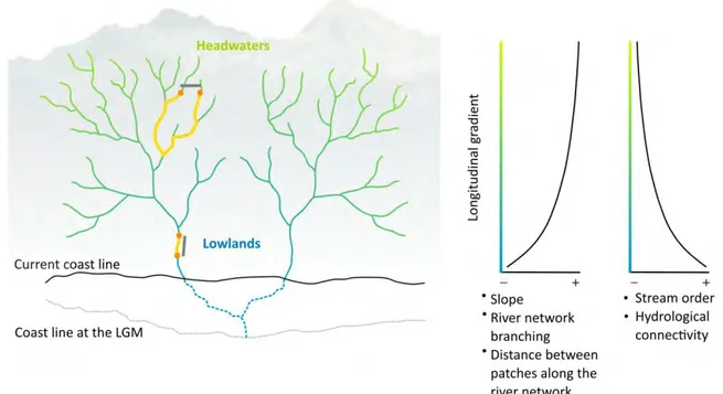
Figure 1. Different features of hydrological connectivity across the longitudinal gradient of schematized river networks. Gradient solid lines represent two river drainages currently disconnected, but that formed a single paleobasin during a lower-sea-level period at the LGM (dashed blue lines). Solid black line shows the current seashore line and the dashed gray line the seashore during the LGM. In a downstream position of the river network, the branching degree is lower and the Euclidian distance between two localities (gray lines) is similar to the distance measured along the river network (yellow lines). As we move to more derivate positions toward headwaters, the dendritic branching increases and the Euclidian distance between two localities can be much shorter than the actual distance through the network (Fagan 2002). This increase in river branching toward headwaters is also accompanied by an increase in river slope that configures changes in habitats along a river drainage basin (Vannote et al. 1980, Benda et al. 2004). This results in a longitudinal gradient of hydrological connectivity that determines the travel distances and dispersal costs for aquatic organisms. On the right side are graphically represented the hydrological connectivity features along the longitudinal gradient.

Strictly freshwater fishes are an ideal model to continue improving our knowledge about the factors and processes that determine species’ geographic range sizes. Indeed, unlike vagile terrestrial organisms, movements and dispersal processes of freshwater fishes are constrained by the dendritic and isolated arrangements of riverine ecosystems at different spatial scales (Fagan 2002, Benda et al. 2004). At the largest spatial scales, fish movements are limited by their inability to cross oceans, high mountain ranges, or expansive lands (Parenti 1991). This implies, for instance, that geographic range expansions between drainage basins are restricted

(38)

37 to geological and hydrological events, such as river captures (Albert et al. 2017) or the confluence of river systems during low-sea-level periods resulting from climatic changes (Dias et al. 2014b). At smaller spatial scales (i.e., within drainage basins), fish movements are determined by a combination of biotic and abiotic factors, including species’ dispersal capacities and behaviors (Radinger and Wolter 2014), the degree of river network branching (Fagan 2002), the basin slope, and other barriers to dispersal (e.g., rapids and waterfalls) that vary longitudinally along the network (Benda et al. 2004) (Fig. 1). As a consequence, drainage basins are structured by gradients of hydrological connectivity, where the branching and type of habitats encountered by species depend on the species’ position within the drainage network, determining the travel distances and dispersal costs for freshwater species (Campbell-Grant et al. 2007, Tonkin et al. 2018) (Fig. 1).

Here we identify the main drivers of geographic range size variation of riverine fishes at global and biogeographic scales. In addition, we explore the complex path system of interactions among these drivers that ultimately determines species’ range size variation. To do so, we compiled the most comprehensive dataset available to date for riverine fish species distributions, including 8,147 species (i.e., 63% of all known strictly freshwater species; Tedesco et al. 2017) covering all continents. Using these distributions, we applied multilevel path models (MLPMs) to evaluate at a global scale the effect of several drivers encompassing the main explanations already proposed for the variation of species’ geographic range size (SI

Appendix, Table S1). This allowed us to determine the direct and indirect effects through

which multiple drivers influence the geographic range size, while controlling for the effect of random factors (i.e., taxonomic relatedness and spatial dependence). We further examined the strength and consistency of these drivers and pathways among the different biogeographic realms of the world.

Results

The range sizes of freshwater fish species varied over six orders of magnitude, from 13 to 10,996,733 km2_{, with a median of 77,322 km}2_{(SI Appendix, Fig. S1). All MLPMs (for global}

and by biogeographic realms) yielded significant coefficients, indicating that the variation in geographic range size was well represented by our path models, and that no links among variables were missing (SI Appendix, Tables S2–S8). The R2_{values of range size for all}

MLPMs ranged between 0.739–0.909 and 0.758–0.921 for the marginal (R2

(39)

38 and conditional (R2

c, fixed plus random factors) variances, respectively (SI Appendix, Table

S9).

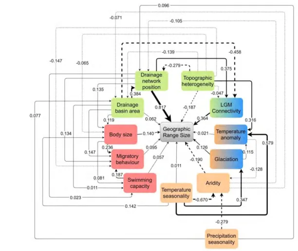
Figure 2. Final path model describing direct and indirect drivers of the geographic range size of freshwater fish species at the global scale. Solid lines indicate positive relationships, and dashed lines indicate negative relationships. Arrows indicate the direction of the relationship. Bold lines indicate the strongest relationships, with line widths proportional to importance. Colors in the boxes show the group of hypotheses to which each predictor belongs: orange boxes represent climatic and energy drivers, blue boxes represent historical drivers, green boxes represent geomorphological drivers, and red boxes represent species traits. Boxes with two colors are drivers belonging to two different groups of hypotheses.

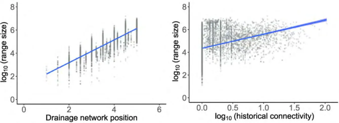
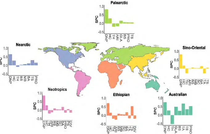
Drainage network position (DNP; the average of the stream orders where a species occurs) and historical connectivity (a measure of past connections among drainage basins) were, by far, the most important drivers of range size variation in freshwater fish species at the global scale (Figs. 2 and 3), both with positive standardized path coefficients (SPC) followed by aridity and topographic heterogeneity showing negative coefficients. Glaciation history and body size were, respectively, the most important historical climatic and species