Numerical modelling of the impact of climate change on the morphology of Saint-Lawrence tributaries

Numerical modelling of the impact of climate change on the morphology of Saint-Lawrence tributaries

par

Patrick Michiel Verhaar

Département de géographie Faculté des arts et des sciences

Thèse présentée à la Faculté des études supérieures en vue de l’obtention du grade de Philosophiæ Doctor (Ph.D.)

en géographie

Février, 2010

c

Faculté des études supérieures

Cette thèse intitulée:

Numerical modelling of the impact of climate change on the morphology of Saint-Lawrence tributaries

présentée par: Patrick Michiel Verhaar

a été évaluée par un jury composé des personnes suivantes:

Jeffrey Cardille président-rapporteur Pascale M. Biron directrice de recherche André G. Roy membre du jury André St-Hilaire examinateur externe Antonia Cattaneo

représentante du doyen de la FES

Cette thèse examine les impacts sur la morphologie des tributaires du fleuve Saint-Laurent des changements dans leur débit et leur niveau de base engendrés par les changements cli-matiques prévus pour la période 2010–2099. Les tributaires sélectionnés (rivières Batiscan, Richelieu, Saint-Maurice, Saint-François et Yamachiche) ont été choisis en raison de leurs différences de taille, de débit et de contexte morphologique. Non seulement ces tributaires subissent-ils un régime hydrologique modifié en raison des changements climatiques, mais leur niveau de base (niveau d’eau du fleuve Saint-Laurent) sera aussi affecté. Le modèle mor-phodynamique en une dimension (1D) SEDROUT, à l’origine développé pour des rivières graveleuses en mode d’aggradation, a été adapté pour le contexte spécifique des tributaires des basses-terres du Saint-Laurent afin de simuler des rivières sablonneuses avec un débit quotidien variable et des fluctuations du niveau d’eau à l’aval. Un module pour simuler le partage des sédiments autour d’îles a aussi été ajouté au modèle. Le modèle ainsi amélioré (SEDROUT4-M), qui a été testé à l’aide de simulations à petite échelle et avec les conditions actuelles d’écoulement et de transport de sédiments dans quatre tributaires du fleuve Saint-Laurent, peut maintenant simuler une gamme de problèmes morphodynamiques de rivières. Les changements d’élévation du lit et d’apport en sédiments au fleuve Saint-Laurent pour la période 2010–2099 ont été simulés avec SEDROUT4-M pour les rivières Batiscan, Richelieu et Saint-François pour toutes les combinaisons de sept régimes hydrologiques (conditions actuelles et celles prédites par trois modèles de climat globaux (MCG) et deux scénarios de gaz à effet de serre) et de trois scénarios de changements du niveau de base du fleuve Saint-Laurent (aucun changement, baisse graduelle, baisse abrupte). Les impacts sur l’ap-port de sédiments et l’élévation du lit diffèrent entre les MCG et semblent reliés au statut des cours d’eau (selon qu’ils soient en état d’aggradation, de dégradation ou d’équilibre), ce qui illustre l’importance d’examiner plusieurs rivières avec différents modèles climatiques afin d’établir des tendances dans les effets des changements climatiques. Malgré le fait que le débit journalier moyen et le débit annuel moyen demeurent près de leur valeur actuelle dans les trois scénarios de MCG, des changements importants dans les taux de transport de sédiments simulés pour chaque tributaire sont observés. Ceci est dû à l’impact important de fortes crues plus fréquentes dans un climat futur de même qu’à l’arrivée plus hâtive de la

crue printanière, ce qui résulte en une variabilité accrue dans les taux de transport en charge de fond. Certaines complications avec l’approche de modélisation en 1D pour représenter la géométrie complexe des rivières Saint-Maurice et Saint-François suggèrent qu’une approche bi-dimensionnelle (2D) devrait être sérieusement considérée afin de simuler de façon plus exacte la répartition des débits aux bifurcations autour des îles. La rivière Saint-François est utilisée comme étude de cas pour le modèle 2D H2D2, qui performe bien d’un point de vue hydraulique, mais qui requiert des ajustements pour être en mesure de pleinement simuler les ajustements morphologiques des cours d’eau.

Mots clés : modèle mophodynamique, fleuve Saint-Laurent, changements climatiques,

transport de sédiments en charge de fond, niveau de base, risque d’inondation, débit efficace, période de récurrence, débit demi-charge.

This thesis investigates the impacts of climate-induced changes in discharge and base level on the morphology of Saint-Lawrence River tributaries for the period 2010–2099. The selected tributaries (Batiscan, Richelieu, Saint-Maurice, Saint-François and Yamachiche rivers) were chosen because of their differences in size, flow regime and morphological setting. Not only will these tributaries experience an altered hydrological regime as a consequence of climate change, but their base level (Saint-Lawrence River water level) will also change. A one-dimensional (1D) morphodynamic model (SEDROUT), originally developed for aggrading gravel-bed rivers, was adapted for the specific context of the Saint-Lawrence lowland tribu-taries in order to simulate sand-bed rivers with variable daily discharge and downstream water level fluctuations. A module to deal with sediment routing in channels with islands was also added to the model. The enhanced model (SEDROUT4-M), which was tested with small-scale simulations and present-day conditions in four tributaries of the Saint-Lawrence River, can now simulate a very wide range of river morphodynamic problems. Changes in bed eleva-tion and bed-material delivery to the Saint-Lawrence River over the 2010–2099 period were simulated with SEDROUT4-M for the Batiscan, Richelieu and Saint-François rivers for all combinations of seven tributary hydrological regimes (present-day and those predicted using three global climate models (GCM) and two greenhouse gas emission scenarios) and three scenarios of how the base level provided by the Saint-Lawrence River will alter (no change, gradual decrease, step decrease). The effects on mean annual sediment delivery and bed ele-vation differ between GCM and seem to be related to whether the river is currently aggrading, degrading or in equilibrium, which highlights the importance of investigating several rivers using several climate models in order to determine trends in climate change impacts. Despite the fact that mean daily discharge and mean annual maximum discharge remain close to their current values in the three GCM scenarios for daily discharge, marked changes occur in the mean annual sediment transport rates in each simulated tributary. This is due to the important effect of more frequent large individual flood events under future climate as well as a shift of peak annual discharge from the spring towards the winter, which results in increased vari-ability of bed-material transport rates. Some complications with the 1D modelling approach to capture the complex geometry of the Saint-Maurice and Saint-François rivers suggest that

the use of a two-dimensional (2D) approach should be seriously considered to accurately simulate the discharge distribution at bifurcations around islands. The Saint-François River is used as a test case for the 2D model H2D2, which performs well from a hydraulics point of view but which needs to be adapted to fully simulate morphological adjustments in the channel.

Keywords: morphodynamic model, Saint-Lawrence River, climate change, bed-material

RÉSUMÉ . . . i

ABSTRACT . . . iii

CONTENTS . . . v

LIST OF TABLES . . . ix

LIST OF FIGURES . . . xi

LIST OF APPENDICES . . . xix

NOTATION . . . xxi

DEDICATION . . . xxv

ACKNOWLEDGEMENTS . . . .xxvii

CHAPTER 1: INTRODUCTION . . . 1

CHAPTER 2: BACKGROUND . . . 5

2.1 The river system. . . 5

2.2 Climate change . . . 11

2.2.1 Past climate change . . . 11

2.2.2 Future climate change . . . 12

2.3 Climate change impact on rivers. . . 13

2.3.1 Past impacts. . . 15 2.3.2 Future impacts . . . 16 2.4 Sediment transport . . . 17 2.5 Numerical modelling . . . 21 2.5.1 1D models . . . 22 2.5.2 2D models . . . 29

2.5.3 3D models . . . 31

2.6 Saint-Lawrence River system . . . 31

CHAPTER 3: A MODIFIED MORPHODYNAMIC MODEL FOR INVESTI-GATING THE RESPONSE OF RIVERS TO SHORT-TERM CLI-MATE CHANGE . . . 37

3.1 Introduction . . . 37

3.2 Study areas. . . 40

3.3 Additions and changes to the model . . . 41

3.3.1 Sand-bed rivers . . . 41

3.3.2 Climate change . . . 45

3.3.3 Tributaries . . . 46

3.4 Assessment of SEDROUT performance . . . 47

3.4.1 Testing SEDROUT adjustments . . . 47

3.4.2 Calibration and validation . . . 49

3.4.3 Long-term simulation. . . 51

3.5 Discussion . . . 52

3.6 Conclusion. . . 54

CHAPTER 4: EFFECTS OF DISCHARGE AND BASE LEVEL CHANGE DUE TO CLIMATE CHANGE ON BED ELEVATION AND YEARLY BED MATERIAL TRANSPORT OF SAINT-LAWRENCE TRIB-UTARIES: A NUMERICAL MODELLING APPROACH . . . 59

4.1 Introduction . . . 59

4.2 Study areas. . . 60

4.3 Methodology . . . 63

4.3.1 Discharge scenarios . . . 64

4.3.2 Base level scenarios . . . 66

4.3.3 Morphodynamic model . . . 66

4.4 Results. . . 70

4.4.1 Validation using topographic comparison . . . 70

4.4.2 Simulations . . . 71

4.6 Conclusion. . . 84

CHAPTER 5: IMPLICATIONS OF CLIMATE CHANGE FOR THE MAG-NITUDE AND FREQUENCY OF BED-MATERIAL TRANS-PORT IN TRIBUTARIES OF THE SAINT-LAWRENCE . . . 89

5.1 Introduction . . . 89 5.2 Methodology . . . 90 5.2.1 Study area . . . 90 5.2.2 Climate scenarios. . . 91 5.2.3 Morphodynamic model . . . 92 5.2.4 Event analysis . . . 93

5.2.5 Effective and half-load discharge . . . 94

5.3 Results. . . 95

5.3.1 Hydrology . . . 95

5.3.2 Sediment transport. . . 97

5.4 Discussion . . . 107

5.5 Conclusion. . . 110

CHAPTER 6: LIMITS OF 1D NUMERICAL MODELLING: THE NEED TO DEVELOP A 2D APPROACH . . . 113

6.1 Complications in 1D modelling of the Saint-Lawrence tributaries . . . 113

6.1.1 Yamachiche River: critical flow . . . 114

6.1.2 Saint-Maurice River: discharge distribution in bifurcations. . . 117

6.1.3 Saint-François River: sedimentation in a channel branch. . . 121

6.2 2D model: H2D2 . . . 123

6.2.1 Model set-up . . . 125

6.2.2 Adapting H2D2 for morphological simulations. . . 126

6.2.3 Saint-François example . . . 129

6.2.4 Discussion . . . 133

CHAPTER 7: GENERAL CONCLUSION . . . 135

7.1 Key findings. . . 135

7.3 Future research. . . 140 BIBLIOGRAPHY . . . 143

2.1 Characteristics of the rivers previously simulated with SEDROUT . . . 30

2.2 Global climate model and GHG-emission scenarios . . . 33

3.1 Characteristics of the Saint-Lawrence and its tributaries . . . 41

3.2 Overview of collected field data.. . . 42

3.3 Velocity comparison between field measurements with ADCP and simula-tions using SEDROUT . . . 50

4.1 Characteristics of the studied tributaries . . . 62

4.2 The influence of the upstream boundary condition (95%, 99% or 101% of transport capacity) on the sediment transport volume at the downstream bound-ary for the Batiscan River. Data are presented in percentage values compared to the upstream boundary condition at 100% transport capacity for three sce-narios: ref (RefQ-RefH), GCM (HadCM3-RefH), base-level (RefQ-0.01m/yr). 67 4.3 The influence of the upstream boundary condition (95%, 99% and 101% of transport capacity) on the difference in bed elevation (m) compared to the up-stream boundary condition at 100% transport capacity in the Batiscan River at the middle reach (7.5–10 km) and downstream reach (0–2.5 km) for three sce-narios: ref (RefQ-RefH), GCM (HadCM3-RefH), base-level (RefQ-0.01m/yr) 67 4.4 The influence of the upstream boundary grain-size distribution (GSD) (95% or 105% of measured D50) on the sediment transport volume at the down-stream boundary for the Batiscan River. Data are presented in percentage values compared to upstream boundary with measured GSD for three scenar-ios: ref (RefQ-RefH), GCM (HadCM3-RefH), base-level (RefQ-0.01m/yr)). . 69

5.1 Discharge (m3/s) associated with recurrence intervals of 1, 2, 5, 10, 20 and 50 years for the three tributaries, based on the present-day (1932–2004) records at gauging stations in the downstream part of the tributaries. QMAM is the mean annual maximum discharge for each series. . . 94

5.2 Percentage of change in mean daily discharge (Qdaily) and mean annual

max-imum discharge (QMAM) for the period 2010–2099 compared to the

RefQ-scenario for three GCMs in each tributary. . . 95

5.3 Half-load discharge (m3/s) for each discharge scenario for each horizon and for the entire simulated period. Half-load discharge is defined as the value above and below which 50% of the total load is transported. . . 99

6.1 Characteristics of selected Saint-Lawrence tributaries. . . 113

6.2 Overview of attempts to solve the critical flow occurring in the Yamachiche model. . . 115

6.3 Distance between cross sections and the ratio of distance over the width. . . 117

6.4 End date of simulations in the Saint-François River. . . 121

6.5 End date of simulations with different values of R for the sediment trans-port distribution in the Saint-François River for the RefQ-0.01m/y scenario. RQs= _(Qs2Q_+Qs2_s3) is given for a discharge distribution that is 70–30%. Qs:out

represents the sediment transport volume at the downstream boundary for the period 2010-2066. . . 123

6.6 Discharge and water level in the Saint-François River for three flow stages.. . . 125

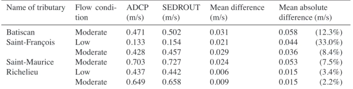
6.7 Mean difference, mean absolute difference, and standard deviation of cross-sectional average velocities between the models (SEDROUT4-M and H2D2) and the ADCP-measurements (m/s).. . . 130

2.1 Balance model for aggradation or degradation of an alluvial river. [Blum and Törnqvist, 2000]. . . 5

2.2 Types of equilibriums based on Schumm [1977]. . . 6

2.3 Overview of interrelationships in the fluvial system. Adapted from Knighton [1998].. . . 7

2.4 Relations between rate of transport, applied stress, and frequency of stress application. Adapted from Wolman and Miller [1960]. . . 8

2.5 The effective discharge for dissolved load, suspended load and bedload. Adapted from Knighton [1998]. . . 8

2.6 Extremes in profile adjustment to continuous base level lowering. Adapted from Bonneau and Snow [1992]. . . 10

2.7 Primary river adjustment (bold arrows) in sand-bed and gravel-bed rivers to changes (+_{: increase,} −_{: decrease) in discharge (Q) and sediment supply}

(Qs). On the left increased discharge or decrease sediment transport. Adapted from Gaeuman et al. [2005].. . . 14

2.8 Mississippi valley terrace sequence from glacial periods. Adapted from Blum and Törnqvist [2000].. . . 15

2.9 Sediment transport classification based origin and mechanism. Adapted from Jansen et al. [1979]. . . . 16

2.10 Shields diagram. Adapted from Buffington [1999].. . . 17

2.11 Schematic illustration of the probability of initial transport according to Grass [1970]. Adapted from Komar [1996]. . . 18

2.12 Flow stress versus grain size diameter. Adapted from Komar [1996]. . . 19

2.13 Sediment distribution at a bifurcation in a river bend highlighting the ’Bulle’-effect. Adapted from De Vriend et al. [2000].. . . 23

2.14 Motion of sediment particle on a transverse slope. Adapted from Engelund [1974] . . . 24

2.15 Stability of nodal point relationship in 1D models, a) unstable bifurcation b) stable bifurcation [Wang et al., 1995]. With H2 and H3 representing the

water depth in both bifurcates, c the power in the nodal point relationship and b the power of the sediment transport formula. Dotted lines indicate phase limits under stationary conditions, continuous lines give possible pathways

of bifurcate depth development. . . 25

2.16 Scheme of nodal point relationship. Adapted from Miori et al. [2006]. . . . 26

2.17 Definition diagram of SEDROUT [Hoey and Ferguson, 1994]. . . 27

2.18 Location of the tributaries of the Saint-Lawrence River. . . 32

3.1 Geographical location of the tributaries of the Saint-Lawrence River. . . 40

3.2 Comparison of the different transport formulae in SEDROUT on the Saint-François River under continuous increasing discharge. Note: the Wilcock and Crowe equation does not predict any sediment transport for this discharge range. 43 3.3 Revised concept of layers in SEDROUT: the centre represents the initial structure, where La is the active layer and Lsubare the sublayers; to the right: update in the case of sedimentation where arrows indicate the direction of deposited sediments. When the uppermost sublayer becomes > 1.5 times the original value, it is subdivided and the lowest layer is erased. To the left: up-date in the case of erosion; far left is the new definition when the uppermost sublayer is < 0. . . 44

3.4 Explanation of the "Channel X" and island simulations used to test the island option in SEDROUT: a) "Channel 0" is used to generate an equilibrium start-ing condition for the test; b) "Channel X" has an island represented by the cross-sectional shape only; c) "Island 1" represents the actual island module. Bold numbers (6,7,8) indicate the position of the island. . . 47

3.5 Comparison between "Channel X" and "Island 1" for a) water level and b) bed level. . . 48

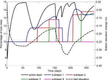
3.6 Variation in the percentage of the smallest grain size class (0.25–0.50 mm) in the new layer module in the active layer and in the four underlying sublayers, as well as in the bed elevation during the simulation at the downstream end of a small-scale model ("Channel 0", Figure 3.4a). . . 49

3.7 Effect of adding a tidal module on a test simulation of the Batiscan River. The y-axis represents the difference between no tide effect and having a water level update every hour (black bars) or every half-hour (white bars). . . 50

3.8 a) Long-term simulation of the Richelieu River, using CSIRO A2 discharge scenario and 0.01 m/y drop in downstream water level, showing yearly sedi-ment transport balance (bars) and annual maximum discharge (line). The sed-iment transport balance values correspond to yearly transport at the upstream boundary minus that at the downstream boundary; b) Cumulative sediment transport balance for a reference scenario (1961–1990 discharge with no wa-ter level drop) and the CSIRO A2 climate scenario with a 0.01 m/y drop. Negative values indicate erosion, whereas positive values indicate deposition.. 52

3.9 Grain size (D50) of the layers at two cross sections in the Richelieu River for

the reference scenario and the CSIRO A2 climate scenario with a 0.01 m/y drop: a) in the centre of the studied reach (at 4.6 km from the downstream limit) and b) at the downstream end.. . . 53

4.1 Location of the studied Saint-Lawrence River tributaries. . . 61

4.2 Long profile of the tributaries based on the deepest point of each cross section (in meters relative to mean sea level) against the distance from confluence with the Saint-Lawrence River or Lake Saint-Pierre, a) Batiscan River; b) Richelieu River; c) Saint-François River, where the dashed line represents the eastern channel along the island; and d) Saint-Maurice River, with a dashed line representing the eastern channel and a dotted line the middle channel continuous line is the main and western channel. . . 63

4.3 Annual bed material transport (m3/year) at the upstream boundary for all the rivers by climate model scenario for the A2 GHG-scenario: a), b), c): Batiscan River; d), e), f): Richelieu River; and g), h), i): Saint-François River. Black lines represent the annual bed material transport of the RefQ scenarios. Filled symbols indicate significant differences compared to the RefQ-RefH scenario at a 5% significance level. Error bars are not presented in this figure to improve readability. . . 72

4.4 Annual bed material transport (m3/year) at the downstream boundary for all the rivers by climate model scenario for the A2 GHG-scenario: a), b), c): Batiscan River; d), e), f): Richelieu River; and g), h), i): Saint-François River. Black lines represent the annual bed material transport of the RefQ scenarios. Filled symbols indicate significant differences compared to the RefQ-RefH scenario at a 5% significance level. Error bars are not presented in this figure to improve readability. . . 73

4.5 Annual bed material transport per horizon at the upstream and downstream boundary for the RefQ-RefH scenario for the three tributaries. Error bars represent +/- one standard error of the variance between years within each horizon. . . 75

4.6 Difference in bed elevation between the 0.01m/y and 0.50m-2040 base level scenarios by the end of 2059. Negative values indicate lower bed elevation in the 0.01m/y scenario. The error bars show +/- one standard error. a): Batiscan River; b): Richelieu River; c): Saint-François River. . . 77

4.7 Difference in bed elevation averaged near the mouth (0.0–2.5 km interval) between the climate model scenarios and the RefQ-RefH scenario, where negative value indicate lower bed elevations: a), b), c): Batiscan River; e), d), f): Richelieu River; and g), h), i): Saint-François River. Filled symbols indicate significant difference compared to the RefQ-RefH scenario at a 5% significance level. Error bars are not presented in this figure to improve read-ability. . . 78

4.8 Difference in bed elevation averaged over a 7.5–10.0 km interval from the river mouth between the climate model scenarios and the RefQ-RefH sce-nario, where negative value indicate lower bed elevations: a), b), c): Batiscan River; e), d), f): Richelieu River; and g), h), i): Saint-François River. Filled symbols indicate significant difference compared to the RefQ-RefH scenario at a 5% significance level. Error bars are not presented in this figure to im-prove readability. . . 79

4.9 Time series showing annual bed elevation variation with discharge for two cross sections, one at the mouth (red) and one in the middle reach (9.4 km upstream from the mouth, in blue) in the Batiscan River for the CSIRO-Mk2 discharge scenario. Continuous lines represent the RefH water level scenario and dashed lines represent the 0.01m/y base-level drop scenario.. . . 80

4.10 Time series showing annual bed aggradation (> 0 m) and degradation (< 0 m) for the 7 reaches in the Batiscan River for a) the reference scenario (RefQ-RefH); b) CSIRO-Mk2 and RefH; c) RefQ-0.01m/y. . . 81

5.1 Dimensionless flood frequency plots expressed as discharge of a given recur-rence interval divided by discharge of a 2-year recurrecur-rence interval in the ref-erence scenario (RefQ), against recurrence interval for a) the Batiscan River; b) the Richelieu River; and c) the Saint-François River.. . . 96

5.2 Annual maximum discharge over the simulated period (2010–2099) for the RefQ and GCM-scenarios for the Batiscan River. Dashed lines refer to the different discharges associated with recurrence interval of 1, 2, 5, 10, 20 and 50, based on the 1932–2004 records at the Batiscan gauging station.. . . 97

5.3 Bed-material sediment transport discharge histograms at the downstream bound-ary for the first (2010–2039) and last (2070–2099) horizons for the Batiscan River (a,d,g,j); Richelieu River (b,e,h,k); and Saint-François River (c,f,i,l) for the RefQ (a,b,c); CSIRO-Mk2 (d,e,f); ECHAM4 (g,h,i); and HadCM3 (j,k,l) models. The arrows indicate the effective discharge for each horizon (black: RefQ, blue: first horizon, green: second horizon and red: third horizon). The upper x-axis represents the present-day recurrence intervals from the 1932– 2004 records. . . 98

5.4 Sediment transport volume as a fraction of the total volume transported with the RefQ-scenario for the a) Batiscan River; b) Richelieu River; and c) Saint-François River. Sediment volumes associated with events where the max-imum discharge is within the same range of recurrence intervals within the scenario are grouped together. For the RefQ-scenario, the present-day (1932– 2004) are used, whereas the future recurrence intervals (2010–2099) are used for each GCM. . . 100

5.5 Boxplots of the relative sediment transport volume per event grouped by present-day recurrence interval of their maximum discharge for: a) Batiscan River; b) Richelieu River; and c) Saint-François River. Whiskers (–) repre-sent the 1% and 99% percentile and symbols (+) reprerepre-sent outliers. Relative sediment transport volume per event is the volume of each individual event divided by the average volume per event for all events in the river concerned. All simulated maximum discharges (i.e. RefQ and GCMs) are combined in this figure. . . 102

5.6 Duration/magnitude diagram of sediment transport event duration against maximum discharge for the Batiscan River. Circles are proportional to the volume of sediment transported during the event. The vertical dashed line indicates the half-load discharge for the RefQ scenario for the 2010–2099 period (509 m3/s). The horizontal dashed line represents the median value of sediment transport event duration (i.e. 50% of the transport events are shorter than this value) in the RefQ scenario (d = 10 days). The percentage in each quadrant gives the contribution to the total sediment transport of short/long and small/large events. The upper x-axis represents the present-day recur-rence intervals. The continuous coloured lines indicate ’envelopes’ of events occurring within each season. a) RefQ; b) CSIRO-Mk2; c) ECHAM4; d) HadCM3. . . 104

5.7 Duration/magnitude diagram of sediment transport event duration against maximum discharge for the Richelieu River. Circles are proportional to the volume of sediment transported during the event. The vertical dashed line indicates the half-load discharge for the RefQ scenario for the 2010–2099 period (1102 m3/s). The horizontal dashed line represents the median value of sediment transport event duration (i.e. 50% of the transport events are shorter than this value) in the RefQ scenario (d = 12 days). The percentage in each quadrant give the contribution to the total sediment transport of short-/long and small/large events. The upper x-axis represents the present-day recurrence intervals. The continuous coloured lines indicate ’envelopes’ of events occurring within each season. a) RefQ; b) CSIRO-Mk2; c) ECHAM4; d) HadCM3.. . . 105

5.8 Duration/magnitude diagram of sediment transport event duration against maximum discharge for the Saint-François River. Circles are proportional to the volume of sediment transported during the event. The vertical dashed line indicates the half-load discharge for the RefQ scenario for the 2010–2099 period (1225 m3/s). The horizontal dashed line represents the median value of sediment transport event duration (i.e. 50% of the transport events are shorter than this value) in the RefQ scenario (d = 6 days). The percentage in each quadrant give the contribution to the total sediment transport of short-/long and small/large events. The upper x-axis represents the present-day recurrence intervals. The continuous coloured lines indicate ’envelopes’ of events occurring within each season. a) RefQ; b) CSIRO-Mk2; c) ECHAM4; d) HadCM3.. . . 106

5.9 Frequency of the number of occurrences per year of five water surface eleva-tions above bankfull level at the upstream boundary for: a) Batiscan River; b) Richelieu River; and c) Saint-François River. Frequency of occurrence is expressed as a percentage of the number of occurrences per year (e.g. 20% is once in 5 years). The bankfull water surface elevations (calculated based on a 2-year recurrence interval) for the Batiscan, Richelieu and Saint-François rivers are 6.47 m, 6.59 m and 7.55 m, respectively. . . 111

6.1 Map of cross section locations in the Yamachiche River. The arrow indicates the position of the hydraulic jump in the simulations. . . 114

6.2 Measured longitudinal profiles of the Yamachiche (in black). Approximation of the theoretical profile in red.. . . 116

6.3 Cross sections in the Yamachiche River downstream (xs 12) and at the loca-tion of the hydraulic jump (xs 13) as well as the addiloca-tional cross secloca-tion that was used in an attempt to solve the hydraulic jump problem.. . . 116

6.5 Complex geometry of the downstream confluence of the Saint-Maurice River with the Saint-Lawrence River. The black lines in the river indicate the thal-weg of the reaches. Numbers give the proportional discharge split at the bi-furcations as simulated with SEDROUT4-M with the ADCP measured split in brackets. Letters indicate two major bifurcations (A, B) and a smaller one (C). . . 119

6.6 The Saint-François River bed topography with the location of detailed figures indicated by black squares. . . 120

6.7 Predicted magnitude of flow velocities by H2D2 for bankfull flow conditions.. 122

6.8 Two different concepts of moving boundaries in 2D modelling, a) classic approach, b) new approach, adapted from Heniche et al. [2000].. . . 124

6.9 Interpolation of echosounder bed topography in Modeleur and the addition of depth contour lines to provide a better interpolation: a) initial interpolation; b) added points and echo sounder data points; c) final interpolation. . . 125

6.10 Overview of variables and constants that need to be exchanged between the different components of H2D2: SVC, CD2D, SED2D. In the upper-left cor-ner the constants are listed and in the centre the variables that are calculated in post-treatment, and not by the modules themselves, are indicated. . . 128

6.11 Comparison of cross-sectional velocities simulated by SEDROUT4-M with H2D2 simulations three different flow stages: a) low flow; b) moderate flow; c) bankfull flow. Line represents regression the equation and R2are given ate the bottom of each graph. . . 130

6.12 Velocity field at low flow conditions (60 m3/s) as simulated by H2D2. . . 131

6.13 a) Ratio of discharge at the bifurcation (large island) for three flow stages as obtained from ADCP measurements, SEDROUT4-M and H2D2 simulations; b) Sediment transport rate at the bifurcation obtained from SEDROUT4-M and H2D2. Q2and Q3are the discharges in the bifurcated channels. . . 132

Appendix I: Accord des coauteurs et permission de l’éditeur . . . I-1 Appendix II: Bed material transport formulae . . . II-1

II.1 Wilcock and Crowe formula . . . II-1

II.2 Ackers and White formula . . . II-2 Appendix III: SEDROUT4-M FORTRAN code. . . III-1 Appendix IV: Example input-files for Saint-François River . . . IV-1

IV.1 Francois.ini . . . IV-2

IV.2 sedfiles.ini . . . IV-5

IV.3 LacStPie.wld . . . IV-6

IV.4 FrEA2010.qdt . . . IV-7

IV.5 Fran2010.sds . . . IV-8

α coefficientAckers and White[1973] equals 10 -βτ direction of shear stress relative to longitudinal direction rad

βsi direction of sediment transport relative to longitudinal direction rad

λ bed porosity

-ν kinematic viscosity of water m2/s

φ grain size class D = 2−φ

-ψ τ_/τri

-ρ density of water kg/m3

ρs density of sediments kg/m3

τ bed shear stress Pa

τri reference shear stress of size fraction i Pa

τrs50 shear stress of Ds50 Pa

θi non dimensional shear stress (Shields number) for size fraction i -1,2,3 subscripts for branches,1 = upstream,2 and3= bifurcates

Ai coefficient

-B channel width m

b power of the sediment transport equation qs∼ aub

-C coefficient

-c power of nodal point relationship

-d exponent

-Da particle size that begins to move under the same conditions as uniform material m

Di grain size of fraction i m

D16 subsurface particle size for which 16% of the sediment sample is finer m

D₅₀ subsurface particle size for which 50% of the sediment sample is finer m

D84 subsurface particle size for which 84% of the sediment sample is finer m

Dgri dimensionless particle size of the ith fraction

-Ds50 median grain size of bed surface m

Dsm mean grain size of bed surface m

e transition exponent

-Ei proportion of volume material in the exchange layer

-Fi proportion of fraction i in surface size distribution

-Fx, Fy resulting momentum in longitudinal and lateral direction _kg·m/s

Fgri mobility number of sediment

-g acceleration due to gravity m/s2

H water depth m

h water surface elevation m

hds downstream water elevation m

k exponent

-La active layer thickness m

Lsub thickness of the first sublayer m

pi proportion of volume material in bedload

-Q water discharge m3/s

q specific discharge m2/s

Qs total sediment transport m3/s

qx longitudinal specific discharge m2/s

qy lateral specific discharge m2/s

qib volumetric bed material transport per unit width of size i m2/s

Qsi total sediment transport of size fracion i m3/s

Q!_si dimensionless sediment transport rate of size fraction i

-R parameter to adjust the sediment transport ratio at a bifurcation

-RQ is the ratio of water discharge at a bifurcation

-RQs is the ratio of sediment transport at a bifurcation

-s ratio of sediment to water density

-t time s U mean velocity m/s u longitudinal velocity m/s u! shear velocity m/s v lateral velocity m/s x longitudinal distance m

Xi rate of sediment transport in terms of mass flow per unit flow rate for the ith fraction g/g/s

y lateral distance m

Ter gedachtenis aan mijn geliefde peetoom Frans van Beek (1938–2009) en peettante Ria van Beek-Mensch (1940–2005). Die zich altijd zeer betrok-ken hebben getoond met mijn leven, die mij ge-steund hebben om dit avontuur aan te gaan en die mij dit graag hadden zien afronden.

In memoriam of my beloved godfather Frans van Beek (1938–2009) and godmother Ria van Beek-Mensch (1940–2005). Who were always very in-volved with my life, who encouraged me to start this adventure and who would have liked to have seen me finish.

Ria:

’blijf lachen’ ’keep laughing’ Frans:

’Zonder verleden geen toekomst’ ’Without past no future’

This thesis was financially supported by an NSERC Strategic Grant and by the Canada Re-search Chair in Fluvial Dynamics (André Roy, Université de Montréal). I would like to thank them to have given me the opportunity to complete my thesis.

Jean Morin and Olivier Champoux, at Environment Canada are greatly thanked for their support and help in setting up the 2D model for the Saint-François River with H2D2, dur-ing two study-visits at their office in Québec City. Also many thanks to Yves Secretan at INRS-ETE, who provided assistance on the initial setup for the incorporation of bed material transport in H2D2 and from whom I learned a great deal about programming in complex software.

The collection of all the field data could not have been done with the great help of Clau-dine Boyer, who coordinated all the field campaigns. Environment Canada is greatly thanked for granting access to their survey boat and equipment – special thanks to Guy Morin for driving the boat and for his helping hand in collecting data in the field. Without the help of the following summer field assistants the collection of data and the treatments would not have been possible, thanks to: Geneviève Ali, Michele Grossman, Francis Gagnon, Jeremy Groves, Olivier Lalonde, and Samuel Turgeon.

The adaptation of SEDROUT was streamlined by the great help of Trevor Hoey, at Uni-versity of Glasgow, who made me become familiar with the code and programming. Rob Ferguson, at Durham University, was a great help along with Trevor to set up the models for the tributaries and to help structuring the analysis. I would like to thank both, Trevor, but in particular Rob, for their contributions to the papers and for their critical and very useful comments.

The input from Ouranos and in particular of Diane Chaumont and Isabelle Chartier is highly appreciated. Their contribution to the papers and their help to respond to comments from reviewers was very useful.

Furthermore, I would like to thank André Roy and Laël Parrot, for their guidance and support throughout my doctorate. Their input and vision were of great value to this thesis. Also I’m grateful for the comments of the committee members: André Roy, André St-Hilaire, Jeffrey Cardille and Antonia Cattaneo. Last, but definitely not least, I could not have finished

this thesis without the great help and support of my supervisor Pascale Biron. The comments, questions, discussions and support were highly appreciated and I’m very glad that her support was not limited to the professional side of fulfilling a thesis and included personal support, opportunism, encouragement and patience.

The personnel of the geography department is thanked for their help in sorting out admin-istrative work for my inscription, study permits and teaching assistantships, merci beaucoup. As with all large projects and especially with the realisation of a doctorate the personal support is also a necessity. Therefore I would like to thank the people close to me who had supported me throughout the project and were there from the beginning on. My parents, dank jullie wel pap en mam voor de motivatie, steun en aan moedigingen, for their encourage-ments, my brother en sister in law, ook jullie bedankt voor alles en ook voor de foto’s van een vrolijk nichtje, ook Caitlin voor de mooie versieringen. My friends back in the Netherlands, for giving feedback, support and being jealous I lived in that lovely place called Montréal: David, Dirk, Frank, Michel and Simon.

Many thanks to my close friends that supported me, dragged me through rough times, and were available to listen to me. Thank you, Luis/Renée/Hernandez, I’ll never forget our ad-ventures in Pierrefonds et les autres ’côneries’.... and of course the introduction to the Latino life style (Rodriguez Sanchez). Viele danke, Matt und Katha for your time, support and com-prehension in difficult times. There are some students from the department I would like to thank, for their help on little problems with computers, courses and programs, but also help-ing me to settle down in Montréal and learnhelp-ing French. First of all the students from the lab: merci beaucoup pour le bonne atmosphère, les discussions et explications Bruce, Géneviève Ali, Géneviève Marquis, Hélène, Jay, Julie, Katherine, Laurence, Mathieu, Michele, Olivier et Rachel. Second the students from the forth floor: Clement, Cristiane, Guillaume, Mélanie (pour assuré que je perde un bon bout de temps pendant mon doctorat et l’aide a apprentis-sage de français) et Rodolphe pour boire du café, de la bière (thirsty Tuesdays), etc. And also a great thanks to my roommates I had over the time for sharing food, friends and just being there: Crystal (best roommates ever!), Nathalie, Simon, Bianca, Ieva, Vidas, Ismaïl, Mélodie, Steve and Max; thanks for all guys!! And many more, but someone needs to know when to stop, once again all thanks for the support, help and distractions (which are also important to survive)!!

INTRODUCTION

Climate change can affect large river systems through variations in discharge and water lev-els. The variation in discharge leads to changes in sediment transport capacity and has po-tential consequences for infrastructures, navigation and flood risk. As the water level of the mainstream is the base level for incoming streams, variation in water level will also have an impact on tributary streams. This research investigates the impacts of various climate change scenarios on five tributaries of the Saint-Lawrence River (Québec) through the use of a one-dimensional (1D) numerical morphological model. The project is novel in its focus on relatively short time scale (∼ 100 years), as very little research has been undertaken to evaluate the possible impacts of short to medium term climate change on river morphology and sediments, despite their potential ecological and economical importance.

Rivers tend to search for equilibrium between external forcing (discharge and water level) and internal dimensions (width, depth, slope, sinuosity, etc.). Changes in discharge and downstream water level can have very large impacts on local river morphology, because of the non-linear character of morphological processes. Morphological response to changes in discharge and/or base level is largely dependent on local settings such as sediment type, bed slope, bank material, etc. Climate changes do not simply result in increasing or decreasing discharge, but they actually alter the shape of the hydrograph, for example with increased spring flow and lower summer discharge. Therefore, a direct derivation of the consequences for sediment transport cannot be made and numerical models need to be used. However, studies that link the effects of future changes in temperature and precipitation to hydrology and river morphology are very sparse [Gomez et al.,2009].

A major issue when dealing with a numerical modelling approach is dealing with the un-certainty of predictions and models. The input for our morphodynamic model comes from prediction of greenhouse gas scenarios that drive global or regional climate models to predict changes in temperature and precipitation, which are then used in a hydrological model to obtain river discharges. These initial steps were carried out by the Ouranos research centre, a consortium on regional climatology and adaptation to climate change [www.ouranos.ca,

Chaumont and Chartier, 2005]. Ouranos is the main source of North American regional climate simulations and, as such, it is recognized as a leading research centre in climate change in Canada that brings together 250 scientists and professionals from different disci-plines. Ouranos is a partner in the NSERC Strategic grant that has funded this project. The discharge scenarios provided by Ouranos were used to force a morphodynamic model that transfers bed shear stress into sediment transport rates. The transformation from discharge to morphological changes is described in this thesis.

The overall objective of this study is to explore the morphological impacts on rivers of near-future climate change. The specific objectives are:

1. To modify and validate a one-dimensional morphodynamic model for the geomorpho-logical context of selected tributaries of the Saint-Lawrence River;

2. To determine how climate-induced changes in near-future hydrology will affect the stability and sediment delivery of tributaries of the Saint-Lawrence River;

3. To determine variations in bed-material transport at the event scale in order to deter-mine the impact of more frequent extreme events on rivers;

4. To explore the potential of two-dimensional (2D) long-term morphological simula-tions.

Chapter2provides the background information on key variables of the river system, cli-mate change, morphological modelling as well as a description of the study area. A general review of these aspects is presented along with a discussion of the past and current knowledge of river adaptation to climate change and prediction/simulation of future climate change ef-fects on precipitation, temperature, discharge and river morphology. The choices of models, study areas and sediment transport formula are justified.

Chapters 3, 4and5correspond to articles that are published in or submitted to interna-tional scientific journals. As such, some repetition occurs to enable the individual publica-tions to be read on their own. These chapters include a detailed methodology for the analysis done within each article. Chapter3describes the choice, modification and validation of the morphological model (SEDROUT) for the selected tributaries. Results of the simulations are presented in chapter4by focusing on yearly average and global trends in the comparison

be-tween scenarios, whereas chapter5examines more closely the event scale in order to address the role of extreme events in river response to climate changes.

Chapter6explains in more detail the problems faced with modelling some of the selected tributaries with a 1D model, namely the Saint-Maurice, Yamachiche and Saint-François rivers. The chapter also explores the use of two-dimensional modelling on one of the selected tributaries (Saint-François River). Because of complexities such as islands, two-dimensional modelling could help resolve the problems faced with the 1D model, despite the increased computational cost. Finally, chapter7provides a general conclusion and directions for future research on the impacts of climate change on river morphology.

The response of a river to changes in discharge and/or base level is complex. Most of the research focuses on one of the two aspects over short time scales or the combination of the two over very long temporal scales. The combination of discharge change and base level change on a near future scale has not been addressed before in geomorphological mod-els. Furthermore, research on near future climate is typically limited to changes in discharge, ecological effects related to changes in habitat or flood risk assessment, based on usually only one climatic scenario. This project will investigate the effects of both a change in discharge and base level on the morphology of the tributaries and the main stream using various sce-narios. Finally, there is a lack of research on climate change on mild slope, sand-bed rivers. Given that most of human settlements around the world are located in the low-land areas of the river system, morphological changes in these areas can have potentially large impacts.

Morphodynamic simulations with discharge scenarios obtained from two different green house gas scenarios and the use of different climatic models are a major strength of this study. Examining different tributaries within the same region also makes this research unique and enhances the potential for generalization of the results. Finally, the intermediate temporal scale (∼100 years) combined with a fairly large spatial scale (around 15 km), also contribute to the originality of this research.

BACKGROUND

2.1 The river system

Figure 2.1: Balance model for aggradation or

degrada-tion of an alluvial river. [Blum and Törnqvist,2000]

Rivers are constantly trying to find an equilibrium state in which there is a bal-ance between the water force and channel resistance [e.g. Schumm, 1977; Leopold and Bull, 1979]. Over intermediate time scales, rivers are in a near equilibrium state where the balance between stream power and sediment transport is almost achieved, which is characterized by a stable lon-gitudinal profile; among others Schumm

[1977] defined this as the graded state. This pseudo equilibrium state is one where the

water slope and bed slope are constant over time although the elevation of the bed and water may change, i.e. aggradation or degradation may occur. Perturbations in water discharge or base level will interrupt this balance and the river system will adjust by finding a new balance between stream power and sediment transport (Figure2.1). Aggradation or degradation of alluvial rivers is thus a result of the balance between sediment supply on one side and sed-iment transport capacity (or stream power) on the other side. However, this model is very general and the effects of the shape of the hydrograph or thresholds for sediment transport are not taken into account.

The river system possesses different types of equilibrium depending on the time scale of interest. As proposed and explained bySchumm[1977], this will vary from the smallest time scale with static equilibrium, meaning a constant bed elevation and continuous sedi-ment transport rate along the river, to a large time scale dynamic metastable equilibrium with episodic erosion (Figure2.2). Time scales in climate research are important, since climatic

parameters like precipitation and temperature are highly dynamic at all time scales, ranging from hours up to more than 100 000 years [Vandenberghe, 1995]. The period of interest is critically important to determine the type of event that is important for landscape evolution [Bogaart and van Balen, 2000]. For example, at scales of hours to days, the dominating events are individual events, like thunderstorms; at scales of months to year, seasonal varia-tions (e.g. snowmelt in the spring); at scales of decades, gradual climate change like global warming; from centuries to millennium, long-term climate oscillations; and at even larger time scales, transition and interglacial cycles. Together all these events shape the landscape and river channels.

Figure 2.2: Types of equilibriums based onSchumm[1977].

A simplification or idealized rep-resentation of the river system can be very helpful to understand the im-portant processes in river systems.

Schumm[1977] divided the river sys-tem in three zones and identified the dominant process in each case. In upstream to downstream order these are: the production zone, the transfer zone and the deposition zone. Ero-sion, transport and deposition of sed-iments occur in all the three zones. However, sediments are generally coming from the upstream region and transported through the middle sec-tion and deposited in the downstream zone. In natural rivers, sediments are not transported to their depositional site at once. During their journey down the river they are stored temporarily in the system as colluvial, alluvial fan or fluvial deposits. These deposits are eroded later on and sediments are transported again.

The river system is considered a complex system [Leopold and Bull, 1979;Hey, 1986;

Knighton, 1998; Phillips, 2003]. In order to be defined as complex, a system must have one or more of the following behaviours: non-linear, unpredictable, multiple equilibrium states, memory and multiple (temporal and spatial) scales. Typical examples of complex

systems are: ecosystems, economies, transportation networks and neural systems [Parrott,

2002]. In the context of complex systems, unpredictability and non linearity refer to multiple equilibrium states that can exist within the system and for which one can therefore not predict the outcome directly. However, it does not imply that the evolution cannot be simulated; it is only impossible, or very hard, to postulate based on general assumptions what equilibrium state will be reached. Numerical models can still be used to evaluate different responses to input parameters, a practice that is often employed in geomorphology, by the evaluation of past events or comparison of different future changes (sensitivity analyses) [Coulthard and Macklin,2001;Hulse et al.,2009]. Conceptual models and numerical morphological models possess a complex non-linear behaviour which is not an artefact of the model, but which is observed in many geomorphic phenomena [Phillips,2003].

Figure 2.3: Overview of interrelationships in the fluvial system. Adapted fromKnighton[1998].

Over the years several attempts have been made to incorporate all the inter-relationships within-river system to be able to predict river response to any change in external forcing or within the river system [e.g.Schumm,1977;Hey,1986;Knighton,1998;Eaton et al.,2004]. Figure2.3provides an overview of these relationships. Although this overview contains all the factors in play, it is difficult to see the impact of a specific change due to the large number of feedback loops. This is the unpredictable aspect as defined above. Ideally, a river system model should include all these inter-relationships, although it is virtually impossible to define all the boundary conditions.

Figure 2.4: Relations between rate of

transport, applied stress, and frequency of stress application. Adapted fromWolman and Miller[1960].

A common assumption in geomorphology is that the median magnitude floods are the most influential in long-term landscape evolution [Figure 2.4 Wolman and Miller,1960]. Effective, dominant, channel form-ing or half-load discharge are the concepts that exist to determine the magnitude and recurrence interval of these floods [Wolman and Miller, 1960;Vogel et al.,

2003;Doyle et al., 2007]. The dominant flood is of-ten associated with bankfull discharge, which is gener-ally true for stable rivers in an unconfined environment [Andrews,1980;Van Den Berg,1995]. The recurrence interval of the bankfull discharge varies among rivers from about 1 year to 32 years depending on their mor-phological state [Wolman and Miller, 1960;Andrews,

1980;Carling,1988;Knighton,1998;Barry et al.,2008]. Long recurrence intervals are most likely found in degrading rivers where banks are high [Knighton,1998]. The most common recurrence interval for bankfull discharge is about 1.5 years [Knighton,1998, among others]. However, it is not always obvious to determine bankfull discharge as the bankfull stage of cross sections may not exhibit a clear limit between the channel and the bank.

Figure 2.5: The effective discharge for dissolved load, suspended load and bedload. Adapted fromKnighton

[1998].

Wolman and Miller[1960] proposed to use a combination of discharge ranges and total volume transported to determine which discharge is transporting the largest volume. The

method was first developed for suspended load in rivers where rating curves of suspended transport were available. However, the idea of effective or dominant discharge has been criticized when generalized towards bedload transport due to the large variability of the mea-surements [e.g.Andrews, 1980;Nash, 1994;Vogel et al.,2003;Doyle and Shields,2008]. In Figure2.5it can be seen that the magnitude of the effective discharge and hence the re-currence interval depends on the type of sediment transport [e.g.Knighton,1998]. Channel dimensions are more related to bedload transport than suspended transport, therefore it seems more likely that the effective discharge is a relatively rare event. The effective discharge is found to vary greatly between rivers [Pickup and Warner, 1976;Ashmore and Day, 1988;

Nash, 1994;Torizzo and Pitlick, 2004]. One of the difficulties with this concept is that it is very sensitive to how the discharge ranges are defined [Crowder and Knapp, 2005] and it relies on sediment rating curves which are mostly not well known for a given river. An alternative approach is the half-load discharge (value above and below which half the long-term sediment load is transported) which is a more robust measure of discharge [Vogel et al.,

2003]. This approach uses the cumulative sediment transport in a similar way to how the median diameter of grain size distribution is determined.

Alluvial rivers will respond to climate change through changes in discharge related to variation of precipitation and evaporation, which will consequently influence discharge mag-nitude, flood frequency and duration [Gibson, 2005; Molnar et al., 2006], and base level [Schumm, 1977; Leopold and Bull, 1979; Tucker and Slingerland, 1997; Blum and Törn-qvist, 2000]. Base level changes are often considered only in terms of sea level variation, especially in climate change and river basin research, but major rivers act as local base lev-els for their tributaries [Slingerland and Snow, 1988;Schumm,1993;Church, 1995]. Both discharge and base level changes have different effects on the river morphology and the pre-diction of the river response for each variable taken individually is difficult as it depends on other factors such as the magnitude, duration and direction of the perturbation [Schumm,

1993;Van Heijst and Postma,2001]. The assessment of the river response to both discharge and base level changes can only realistically be done by numerical modelling.

Base level, as defined byPowell [1875], is used to identify the elevation to which rivers or landscape will erode. Essentially this level is the sea level, although it is known that rivers will erode slightly below it [Schumm, 1993]. Base level is also defined as the local level to which rivers erode, for instance the water level in the main stream or in a lake, or the

bed rock in degrading rivers. Therefore, the water level in the Saint-Lawrence River is the base level for all its tributaries. A base level change is often viewed as a perturbation that occurs in a short reach, which may affect the reaches upstream [e.g.Leopold and Bull,1979;

Begin et al.,1981;Bonneau and Snow,1992]. However, the upstream distance influenced by the base level change cannot easily be determined beforehand [Blum and Törnqvist,2000]. Some studies show that the base level in the main stream is only affecting the tributaries locally [Leopold and Bull,1979]. On the contrary,Slingerland and Snow[1988] simulated the response of a river network to a lowering of its base level. Flow in the tributaries was in the order of 10% of the discharge in the main stream. The response of the system was cyclic, with periods of erosion and sedimentation in the main stream, due to a change in the input of sediment in the main stream by erosion of the tributary. The type of response to a base level lowering also depends on the rate of base level change [Bonneau and Snow,1992].

Figure 2.6: Extremes in profile adjustment

to continuous base level lowering. Adapted fromBonneau and Snow[1992].

A slow rate will lead to a period of initial steepening of the channel followed by parallel erosion (Figure2.6a). Continuous steepening occurs when the rate of change is higher than the response of the head waters. A slow rate of base level change allows the river to adjust its pattern and maintain its slope, whereas a higher rate leads to incision [Schumm, 1993]. The type of re-sponse is also highly dependent on local settings and controls. According toSchumm[1993] classification, base level controls are direction, magnitude, rate and duration; geological controls are lithology, structure and nature of valley alluvium, and geomorphic con-trols are inclination of exposed surface, valley mor-phology, river morphology and adjustability.

A river has several degrees of freedom to respond to changes in discharge and base level, namely bed el-evation, channel width, channel depth, meander wave length, sinuosity, bed slope, width to depth ratio and bed composition [Knighton,1998;Eaton and Church, 2004]. Schumm[1977] developed a simplified river model that described the direction of change for all these variables as a function of change in discharge and sediment

transport rate. His river model, however, only gives a qualitative description of the expected changes.Schumm[1993] also argued that the main response of an unconfined sand-bed river to a change in base level is a change in river pattern [Simon and Hupp,1986;Simon,1989,

1992]. However, field studies such asBegin et al.[1981] show that this is not necessarily the case and that the river response can be more in terms of incision when a base level lowering occurs. Discrepancies in the type of response between rivers may also be related to sedi-mentology, as rivers with cohesive sediment will erode their banks [Schumm, 1993;Doyle and Harbor, 2003]. However, a case study in the Jordan River revealed that non-cohesive sediments also underwent incision as a primary response to base level lowering [Hassan and Klein,2002], so other variables must intervene in river adjustment. For example, the slope of the continental shelf, in the case of sea level change, plays a role in the river response [ Sum-merfield,1985;Blum and Törnqvist,2000]. When the slope of the continental shelf is steeper than the river channel slope, incision and increased sinuosity are the most likely responses. If the slope of the continental shelf is less steep, then aggradation or channel straightening will occur. When the slopes are the same, the river will maintain its sinuosity and there will be no change in sinuosity further upstream.

2.2 Climate change

2.2.1 Past climate change

Climate is an important factor on the evolution of landscape and rivers. It is known that climate gradually changes over time in cycles. Since the last glacial period the earth temperature rise caused the ice caps to melt and the sea level to rise by about 120 m over that period [IPCC,2007]. Since the beginning of the Holocene, about 12 000 years ago, the Earth temperature and precipitation have been fairly constant relative to the glacier inter-glacier cycle [e.g.Antoine,2003].

Resolving what happened in the past is often seen as a necessity for future predictions [Dearing et al.,2006]. Unfortunately, records of past climate are influenced by human activ-ity. Therefore, the reconstruction of climate can only be done when climate, human activities and earth processes, including their interactions are reproduced at all locations and scales [Dearing,2006].

(for example, in ice cover) all over the world. Various records of ice cores and tree ring data indicate that greenhouse gas (GHG) concentrations and global temperature are rising due to human activity. The effect of changing GHG concentrations in the atmosphere varies around the globe and contributes to more extreme meteorological events, like hurricanes, heat waves, etc. [Goudie,2006;Hansen et al.,2006, and references herein]. The global trend is that the earth surface temperature is increaseing over the last decades.

Changes in climate over several decades have been recorded in some watersheds, for ex-ample the Waipaoa River in New Zealand [Gomez et al.,2009]. The evaluation of river basin sediment transport as a consequence of these changes is complicated by the other changes within the river basin, such as forest clearing, hydraulic structures, etc. Recent climate changes have also been observed in Québec. Over a 44 year period from 1960 to 2003 the temperatures increased between 0.5◦C and 1.2◦C with a strong East-West gradient because of large water bodies in the East [Bourque and Simonet,2008]. Other indicators such as the length of the frost-free season, growing degree-days and heating degree-days have changed over the last decades as well.

2.2.2 Future climate change

There is now a clear consensus that the global climate will continue to change in the near future, at least partly because of human activities [IPCC,2007]. Human activities have greatly increased concentrations of greenhouse gases, such as carbon dioxide and methane. These elevated concentrations will result in higher mean temperature of the earth, however on a regional scale it will alter temperature (increase or decrease) and precipitation which inevitably also affects hydrological systems and river flows [Graham et al., 2007;Minville et al.,2008]. For the assessment of climate change on temperature and precipitation a good understanding of the global interactions of GHG concentrations with temperature and precip-itation is necessary. Furthermore, an estimation of the future GHG emissions is required.

Over the last decades intensive research on both the emission rates and the interaction on global and regional scale have been carried out [IPCC,2007]. The results of these exercises are surrounded by relatively large error margins, not only because of the difficulty of predict-ing future emission rates, but also due to the relatively poor understandpredict-ing of the processes involved. Furthermore, predictions of temperature and precipitation are based on a cascade of modelling steps from GHG emission rates, through global or regional climate modelling.

Predictions on global climate modifications need to be translated to regional changes in order to foresee the effects within watersheds. Different methods for this translation are available, of which the perturbation or delta method is the most widely used [Graham et al.,

2007]. The perturbation method uses a reference period (mostly 1961-1990) for precipitation and temperature and calculate delta values for each season for one representative year in the future. These delta values are then applied to the reference time serie to produce estimates for the future period(s). Although other approaches such as downscaling or runoff routing are increasingly being used, each method has its own limitations [Rosberg and Andréasson,

2006; Graham et al., 2007; Rydgren et al., 2007; Quilbé et al., 2008]. The advantage of the perturbation method is that it is simple, stable and robust and it represents very well changes in mean precipitation and temperature. However, individual events are captured less accurately than in the other available methods [Rosberg and Andréasson, 2006]. Based on direct comparison of downscaling with the delta method byHay et al.[2000] it was concluded that due to uncertainties in GCM’s ability to simulate current conditions, future impacts of both methods remain questionable.

Overall, it is expected that in Québec for the period 2010–2099 the mean temperature will increase, especially in the cold season [Bourque and Simonet,2008]. For the winter and spring seasons, the precipitation would also increase. As a consequence, the discharge regime of rivers within the province of Québec should change [Chaumont and Chartier,2005]. Al-though the mean annual discharge remains close to current values, the timing of spring floods will change drastically [Boyer et al.,2009].

2.3 Climate change impact on rivers

Fluvial response to climate change has been a topic of study in fluvial geomorphology for many decades. Most of these studies look at historical changes in climate and try to match known climatic events with stratigraphic records, based on the principle that we can learn from the past about present and future climate-human-environment interactions [Blum and Törnqvist,2000;Dearing,2006]. Looking at long time scales (20 000 years), these periods are still relative short compared to an entire glacial and interglacial cycle of about 100 000 years. Over these long time scales sea level (base level) is linked with climate as sea level high stands are linked with warm periods, and lows in sea level are associated with cold

periods.

A climate-induced change in discharge is almost always accompanied by a change in sediment transport [Schumm, 1977]. The effect of such a combined change is different in rivers with a sand bed than in gravel-bed rivers [Gaeuman et al.,2005]. In Figure2.7, it can be seen that the primary response for sand-bed rivers is an adjustment of the bed elevation, whereas gravel-bed rivers will adjust primarily through width. Observations from field data [Gibson,2005] show that it is difficult to isolate the effect of climate change on rivers as it happens in a continuous changing landscape and changes in discharge and sediment transport occur concurrently [Schumm, 1993]. Bogaart and van Balen[2000] use a numerical model to investigate the effects of changes in water discharge and sediment supply. They compared the results of a simultaneous variation of the discharge and sediment supply, with a time lag between the maximum discharge and maximum sediment supply, and they found that the change itself is not as important as the phase-lag between them. The phase lag between dis-charge and sediment supply varies between different river basins, and therefore the response is different for each river.

Figure 2.7: Primary river adjustment (bold arrows) in

sand-bed and gravel-bed rivers to changes (+: increase,

−_{: decrease) in discharge (Q) and sediment supply (Qs).}

On the left increased discharge or decrease sediment transport. Adapted fromGaeuman et al.[2005].

Climate-change related studies on rivers mostly focus on reproducing historical data [e.g. Blum and Törnqvist, 2000; Bogaart and van Balen, 2000; Hassan and Klein,

2002;Molnar et al.,2006]. Because of the importance of the anticipated near-future climate changes, some simulations are in-creasingly being used to assess the impacts on discharges, water levels and economi-cal (navigation, hydro-power or water re-sources) or ecological aspects (e.g. river habitats) [Morin and Côté, 2003; Gibson,

2005; Fowler et al., 2007]. These studies mostly use a worst-case scenario approach. Because of the complexity of river re-sponses described above, even if a simplified approach is used, the type of response to a sin-gle climatic perturbation is often not clear. Field studies, laboratory experiments and models

have been used to generalize river behaviour and analyse equilibrium states [Schumm,1977;

Rhodes,1987;Howard,1988;Bonneau and Snow,1992;Van Heijst and Postma,2001]. But despite all the efforts made to generalize findings, river responses are strongly related to local settings and therefore no general rule exists. Furthermore, the situation is complicated by the large number of degrees of freedom in a river system [Hey,1986;Knighton,1998] and the fact that response is dependent on the flow history [Rhodes,1987;Phillips,2003]. This complexity is illustrated by the study ofVeldkamp and Tebbens[2001] which simulated cli-mate and base level change for the river Meuse and found that preserved fluvial sedimentary records did not relate to neither climate change nor to sea-level change in the lower reaches of the river basin. Furthermore, the link between climate change and river response remains difficult to establish [Vandenberghe and Maddy,2001;Bogaart et al.,2003], at least in part because the uncertainty in the input variables for river response models includes uncertainty in both outputs of climate models and of hydrological models used to convert changes in temperature and precipitation into river discharge [Graham et al.,2007].

2.3.1 Past impacts

There are several studies linking past impacts of climate change to river morphology [e.g.

Blum and Törnqvist, 2000; Bogaart and van Balen, 2000; Knox, 2000;Vandenberghe and Maddy,2001;Adel,2002]. For example,Blum and Törnqvist[2000] were able to summarize the general history of climate change (precipitation and sea-level change) on the Mississippi River valley, over a series of glacial periods (Figure2.8).

Figure 2.8: Mississippi valley terrace sequence from

glacial periods. Adapted from Blum and Törnqvist [2000].

To better understand the relationship between climate and the stratigraphic record, physical and numerical modelling studies has been conducted [Tucker and Slingerland, 1997; Syvitski et al., 1998;

Veldkamp and Tebbens,2001;Bonnet and Crave,2003]. The advantage of these stud-ies is that effects of discharge change or base level can be isolated.Bogaart and van

Balen [2000] show that there is no link in the downstream part of the River Meuse with climate or base-level changes. However,Antoine[2003] revealed that some fluvial systems