Introduction G´en´erale 1 1 On the improvement of the performances of an observer:
A discrete linear system 13
1.1 Introduction . . . 14
1.2 Problem statement . . . 15
1.3 On the properties of the set M . . . . 17
1.3.1 Preliminary results . . . 17
1.3.2 On the accessibility of the set M . . . . 18
1.3.3 An algorithmic approach . . . 21
1.4 observer initial state design . . . 22
1.5 Numerical simulation . . . 26
1.6 Discrete-time delayed system . . . 29
1.7 Conclusion . . . 35
2 A Quadratic Optimal Control Problem for a Class of Linear Discrete Distributed Systems 40 2.1 Introduction . . . 41
2.2 Some useful properties . . . 44
2.3 The optimality system . . . 46
2.4 Convenient topology . . . 48
3 On the controllability for a Biological System :
A compartment Model Approach 60
3.1 Introduction . . . 61
3.2 Mathematical Modelling of the problem . . . 63
3.3 Linear quadratic optimal control . . . 75
3.3.1 Preliminary properties . . . 75
3.3.2 An adequate topology . . . 78
4 Un r´esultat sur la robustesse de la contrˆolabilit´e : Cas de dimension finie 84 4.1 Introduction . . . 85
4.2 Robustesse par rapport `a la dynamique A . . . 86
4.3 Robustesse par rapport `a la matrice de contrˆole . . . 88
4.4 Syst`emes avec commande retard´ee . . . 89
4.4.1 contrˆolabilit´e . . . 89
4.4.2 Robustesse . . . 94
5 Semi-continuit´e inf´erieure d’une fonctionnelle int´egrale 98 5.1 Propri´et´e de type ”Lower closure theorem” pour les ´epigraphes. . . 99
5.2 Semi-continuit´e inf´erieure des fonctionnelles int´egrales. . . 110
5.2.1 Cadre de travail et notations. . . 111
5.2.2 Extension du th´eor`eme de Ekeland-Temam. . . 111
5.2.3 Extension du th´eor`eme de Ioff´e en dimension infinie. . . 115
INTRODUCTION GENERALE
S’inscrivant dans le cadre d’une coop´eration entre l’´equipe d’analyse convexe et optimisation de la facult´e des sciences de Rabat et l’´equipe d’analyse et contrˆole des syst`emes de la facult´e des sciences de Ben M’sik Casablanca, le pr´esent travail, et de mani`ere naturelle, est compos´e de deux parties. La premi`ere partie est consacr´ee `a l’´etude de certains aspects de la th´eorie des syst`emes. Dans la deuxi`eme partie, nous pr´esentons quelques r´esultats, en dimension infinie, sur la semi continuit´e inf´erieure d’une fonctionnelle int´egrale.
L’analyse et le contrˆole des syst`emes est un domaine de recherche d’actualit´e qui ne cesse de susciter l’int´erˆet des scientifiques, cette discipline a connu ses premiers d´eveloppements apr`es la seconde guerre mondiale, ses applications ont eu un impact tr`es positif dans le domaine de l’a´eronautique et de la dynamique du vol ainsi que dans toutes les industries modernes ou le facteur ”rentabilit´e” constitue la pr´eoccupation principale. En automatique, le contrˆole optimal s’est av´er´e ˆetre le meilleur support math´ematique. Actuellement et avec le d´eveloppement des ordinateurs, les applications du contrˆole optimal touchent `a toutes les sciences de l’ing´enieur: communications, robotique, m´et´eorologie, oc´eanographie, g´enie des proc´ed´es, industrie pharmaceutique, industrie de l’automobile, etc.
Depuis une quinzaine d’ann´ees, l’´equipe d’analyse et contrˆole des syst`emes de la facult´e des sciences de Ben M’sik Casablanca s’est beaucoup int´eress´ee aux syst`emes discrets (voir [22], [33], [34], [39],[48], [57], [58], [59], [60], [61], [62], [63], [64], ...). Pourquoi les syst`emes discrets?
- Tout d’abord, un bon nombre de syst`emes sont de nature discr`ete.
- A chaque fois qu’un calculateur fait partie du contrˆole d’un syst`eme, l’´echantillonnage de ce dernier, devient une ´etape n´ecessaire.
- L’analyse et le contrˆole d’un syst`eme, sous sa version discr`ete, est souvent appr´eci´ee par l’ing´enieur et l’automaticien car elle lui ´epargne certaines complications math´ematiques comme le choix de l’espace et la r´egularit´e de la solution.
La litt´erature sur les syst`emes discrets est riche, abondante et diversifi´ee, `a ce titre on peut voir [7], [8], [16], [23], [24], [28], [29], [30], [31], [35], [36], [37], [38], [40], [45], [53], [54], [55], [68] et [69], etc.
Pour contribuer dans cette th´ematique, nous consacrons le premier chapitre [27] de cette th`ese `a l’am´elioration de l’observateur de Luenberger ([43], [44]). Plus pr´ecis´ement, nous consid´erons le syst`eme discret
½
xi+1 = Axi+ Bui , i ≥ 0
x0 ∈ Rn
augment´e de la sortie
o`u x0 ∈ Rn est suppos´e mal connu, xi ∈ Rn, ui ∈ Rm et yi ∈ Rq sont, respectivement,
la variable d’´etat, la variable de contrˆole et la variable de sortie, tandis que A, B et C sont des matrices constantes de dimensions appropri´ees.
L’observateur classique de Luenberger consiste `a d´eterminer une dynamique ½
zi+1= F zi+ Dyi+ P ui , i ≥ 0
z0 ∈ Rp (1)
o`u zi ∈ Rp et F, P et D des matrices constantes de dimensions appropri´ees et v´erifiant
lim
i→∞(zi− T xi) = 0
T xi signifient les composantes de xi `a estimer.
Conscients du fait que la lenteur de la convergence de l’erreur d’estimation kzi− T xik
vers 0 peut ˆetre destructrice pour certains syst`emes, nous proposons, sous certaines conditions, une classe d’´etats initiaux z0 tel que, initialis´e par de tels z0, l’observateur
(1) permet d’atteindre la performance
kzi− T xik ≤ αi , ∀i ≥ 0
o`u (αi)i≥0est une vitesse de convergence fix´ee au d´epart et appropri´ee selon le contexte.
Dans le deuxi`eme chapitre [65], nous nous int´eressons `a la r´egulation d’une classe de syst`emes discrets `a param`etres r´epartis comme suite naturelle `a deux travaux ult´erieurs o`u on a ´etudi´e le probl`eme de r´egulation avec ´etat discret et commande discr`ete [58], et la r´egulation avec ´etat continu et commande discr`ete [21], le travail, sujet de ce chapitre, consiste `a minimiser une fonctionnelle quadratique associ´ee `a un syst`eme distribu´e avec ´etat discret et commande continue dans le temps. Pour plus de d´etails, nous nous int´eressons `a l’optimisation du crit`ere
J(u) =< xN−xd, G(xN−xd) > + N −1X i=1 < xi−ri, M (xi−ri) > + Z T 0 < u(θ), Ru(θ) > dθ o`u (xi)i est la solution de l’´equation diff´erence
xi+1= Φxi+ Z ti+1 ti Bi(θ)u(θ)dθ, i ≥ 0 x0 ∈ X , (2)
o`u xi ∈ X est la variable d’´etat, u(θ) ∈ U est la variable de contrˆole. X et U sont des
espaces de Hilbert, Φ ∈ L(X ), u ∈ L2(0, T ; U) et B
i(.) ∈ L2(0, T ; L(U; X )) pour tout
Le probl`eme de r´egulation mod´elis´e par la minimisation de la fonctionnelle J est ´equivalent `a la d´etermination de la loi de contrˆole u permettant de r´ealiser les objectifs xd ' xN, (xi)1≤i≤N −1 ' (ri)1≤i≤N −1 et ceci `a moindre coˆut. L’originalit´e de ce travail
r´eside dans le mod`ele (2).
En effet, il est connu (voir par exemple [40], [49] and [56]) que la discr´etisation d’un syst`eme continu
x(t) = S(t)x0+
Z t
0
S(t − r)Bu(r)dr, t ∈ [0, T ]
o`u x0, x(t) ∈ X , (S(t))t≥0est un semi groupe fortement continu sur X et B ∈ L(U, X ),
se base sur l’hypoth`ese
u(t) = ui, ∀t ∈ [ti, ti+1[, (3)
et conduit `a la version discr`ete
xi+1= Φxi+ Bui i ≥ 0
avec Φ = S(δ) and B = Z δ
0
S(τ )Bdτ . L’hypoth`ese (3) qui est `a la base du proc´ed´e de discr´etisation (d´ecrit ult´erieurement) devient illogique et aberrante lorsque le contrˆole u est `a variations rapides ou lorsque l’amplitude de temps ti+1− ti est assez grande.
Notre apport consiste donc `a se passer de l’hypoth`ese (3) d’o`u la version discr`ete (2). Pour la d´etermination de l’optimum u∗, nous avons adopt´e une approche structurelle
bas´ee sur l’introduction d’une nouvelle topologie Hilbertienne. De fa¸con similaire `a la m´ethode HUM (Hilbert Uniqueness Method) (voir Lions [41], [42]), nous montrons que l’optimum ainsi que le coˆut optimal d´erivent de l’inversion d’une isom´etrie et qu’ils sont facilement calculables par la m´ethode num´erique classique de Galerkin.
Toujours dans le cadre de l’analyse et contrˆole des syst`emes, nous nous int´eressons dans le troisi`eme chapitre [26] de cette th`ese `a un probl`eme qui rel`eve de la biomath´ematique. Autrement dit, nous consid´erons un mod`ele `a compartiments r´egissant les ´echanges d’une substance entre les diff´erents organes (ou compartiments) d’un corps vivant. D´esirant atteindre un ´etat pr´ed´efini `a un instant donn´e, nous d´eterminons la meilleure strat´egie de contrˆole permettant d’atteindre l’objectif et ceci avec un coˆut minimal. Pour plus de pr´ecisions, nous adoptons dans ce troisi`eme chapitre le mod`ele `a compartiments
½
˙x(t) = Ax(t) + B1u(t) + B2v(t) 0 ≤ t ≤ T
x(0) ∈ Rn
A ´etant la dynamique du syst`eme et qui caract´erise les ´echanges entre les diff´erents compartiments xi du vecteur x(t) = (x1(t), ..., xn(t))T, B1 et B2 d´ecrivent les
com-partiments accessibles et d´esign´es pour ˆetre contrˆol´es, la commande u(t) d´esigne une action discr`ete (qui peut ˆetre une prise de comprim´es ou une injection) et la commande v(t) d´esigne une action continue (qui peut ˆetre un s´erum ou une perfusion). Nous ´etablissons sous des conditions de type Kalman, le contrˆole permettant le transfert du syst`eme et ceci `a moindre coˆut. Dans le cas o`u l’hypoth`ese de Kalman n’est pas satisfaite, au lieu de consid´erer le probl`eme comme ´etant un probl`eme de contrˆolabilit´e, nous l’abordons sous une version plus faible, c’est `a dire nous le traitons comme un probl`eme de r´egulation. La m´ethode H.U.M a ´et´e utilis´ee avec succ`es, pour ´etablir l’optimum ainsi que le coˆut optimal.
Dans le chapitre 4, nous montrons la robustesse de contrˆolabilit´e d’un syst`eme lin´eaire `a param`etres localis´es, c’est `a dire, nous montrons que des petites perturba-tions sur la dynamique du syst`eme ou sur l’op´erateur du contrˆole, n’affectent pas la propri´et´e ”contrˆolabilit´e”, les r´esultats obtenus ont ´et´e ´etendus au cas des syst`emes avec contrˆole affect´e d’un retard.
Vers le d´ebut des ann´ees 70, le probl`eme historique du calcul des variations a ´et´e ramen´e `a l’´etude des fonctionnelles int´egrales et des propri´et´es des espaces int´egraux-diff´erentiels. Depuis, de nombreux chercheurs de plusieurs ´ecoles de tradi-tion math´ematique, russe, fran¸caise, polonaise, italienne et allemande ont ´enorm´ement travaill´e et produit sur le sujet. Nous donnons `a la fin de cette introduction une bibliographie assez repr´esentative de l’´evolution de ces travaux. Une fonctionnelle int´egrale est un op´erateur sur un espace int´egral (ou un produit d’espaces int´egraux) de la forme If(u) =
R
f (u)dµ, la fonction f s’appelle int´egrande. L’un des probl`emes qui ont retenu l’attention, puisqu’il constitue la cl´e pour l’existence de minimum de la fonctionnelle du calcul de variation, est celui de la semi-continuit´e inf´erieure de la fonctionnelle int´egrale. C’est `a cet aspect que nous nous int´eressons dans ce travail. De fa¸con plus pr´ecise, ´etant donn´es deux espaces de Banach X et Y et deux espaces int´egraux LX et LY, nous donnons des conditions pour que la fonctionnelle
If(u, v) =
R
Ωf (ω, u(ω), v(ω))dµ(ω) soit s.c.i sur le produit LX × LY. Ici Ω est un
espace mesurable muni d’une mesure µ, et les fonctions u et v appartiennent aux espaces int´egraux LX et LY qui peuvent ˆetre par exemple L1 l’espace des fonctions
Bochner int´egrables , Lp l’espace des fonctions p-int´egrables, Lϕ l’espace d’Orlicz
associ´e `a un int´egrand normal ϕ, W1,p l’espace de Sobolev ou plus g´en´eralement des
sous-espaces d´ecomposables l’un muni d’une topologie de type forte le second d’une topologie de type faible.
L’objectif de la deuxi`eme partie (chapitre 5 [15]) est de d´egager des condi-tions n´ecessaires et suffisantes pour que If(., .) soit s´equentiellement semi continue
inf´erieurement (s´equentiellement sci) lorsque les espaces X et Y sont de dimension infinie. Ce probl`eme a ´et´e motiv´e principalement par les besoins de la th´eorie de l’existence dans le calcul des variations et le contrˆole optimal des syst`emes `a param`etres distribu´es et dans les in´egalit´es hemi-variationnelles. Une description d´etaill´ee des re-lations entre ces probl`emes en dimension finie pourait ˆetre trouv´ee dans une ´etude de Olech [50].
Notre propos ne se restreint pas aux situations types du calcul des variations et du contrˆole optimal o`u les fonctions u (.) et v (.) sont mutuellement d´ependantes, fr´equemment, v (.) est une collection de d´eriv´ees de u (.). C’est le cas par exem-ple o`u F (u) = RΩf (∇u(ω))dω dont le probl`eme d’optimisation associ´e est inf F (u) : u ∈ W1,p(Ω, Rm); Ω ´etant un ouvert born´e de Rn.
En ´elasticit´e, Ω repr´esente la configuration de r´ef´erence occup´ee par un mat´eriau ´elastique et F l’´energie ´elastique associ´ee au mat´eriau, si F n’est pas semi continue inf´erieurement, en g´en´eral, le probl`eme de minimisation ci-dessus n’admet pas de so-lution. Ce qui met l’accent encore une fois sur l’importance d´eterminante de la s.c.i dans la th´eorie du calcul de variation et de l’optimisation.
Dans notre cas, les fonctions u et v sont ind´ependantes et peuvent appartenir `a deux espaces diff´erents. Dans l’´etude de la s.c.i des fonctionnelles et la th´eorie d’existence, plusieurs auteurs (`a titre d’exemples [9], [17], [18], [19], [20], [25], [32],[50], [52]) ont adopt´e cette hypoth`ese depuis longtemps pour ´eviter ainsi de s´erieuses complications techniques inutiles, d’autant plus qu’elle est souvent v´erifi´ee dans les applications pra-tiques (voir Ioff´e [32]).
En analyse int´egrale, plusieurs propri´et´es de sci des fonctionnelles int´egrales correspon-dent par d´esint´egration `a des propri´et´es qui portent sur les int´egrandes correspondantes , citons pour m´emoire le contrˆole de la r´egularit´e topologique par des conditions de croissance, propri´et´es ´etudi´ees notamment par [10], [11], [12], [13], [14], [51], etc. Notre travail est une suite naturelle d’une s´erie de travaux entrepris dans ce sens dont les premiers datent de plusieurs d´ecennies, notamment ceux de Lebesgues, Hilbert et Tonelli [67], Morrey [46], [47], Reshetnyak [66]. Ces auteurs ont trait´e les cas o`u les fonctions u et v sont `a valeurs dans R ou Rn, Ω un ouvert de R ou Rnmuni de la mesure
de Lebesgues et l’int´egrande f est r´estreinte `a soit |.| soit |.|p. Plus tard, Ekelend et
Temam dans [25] ont ´etabli un r´esultat de semi continuit´e inf´erieure de ces fonction-nelles int´egrales dans le cas o`u f est positive et u et v `a valeurs dans Rn. Cesari [18],
[19] a ´etudi´e la sci de ces fonctionnelles int´egrales en relation avec d’autres r´esultats de fermeture faible en dimension finie, la fonction f est `a valeurs r´eelles, continue et convexe par rapport `a la deuxi`eme variable et Ω v´erifie une hypoth`ese de compacit´e de type Carath´eodory. Olech [51], [52] a introduit des conditions de croissance pour caract´eriser cette sci. Ioff´e [32] a g´en´eralis´e dans le cas o`u (u, v) ∈ L × M o`u L et M sont des espaces int´egraux et les fonctions sont `a valeurs dans Rn et v´erifiant une
condition suppl´ementaire de compacit´e faible `a la place de l’hypoth`ese de positivit´e de f de Ekelend-Temam [25]. Les travaux de Balder [1], [2], [3], [4], [5], [6] ont ´et´e nombreux dans ce sens. Ainsi dans [4], Balder a g´en´eralis´e en dimension infinie les
r´esultats de Olech en se basant sur la notion de seminormalit´e.
Notre contribution consiste `a g´en´eraliser les r´esultats de [25] et [32] au cas de la dimen-sion infinie et sans aucune condition sur Ω. Nos hypoth`eses restent similaires `a celles de la dimension finie . Nous utilisons les mˆemes outils que ceux de [25] et [32], `a savoir le lemme de Fatou, le th´eor`eme de Mazur et une variante du th´eor`eme de Carath´eodory. Ce th´eor`eme n’est valable qu’en dimension finie, obstacle de taille qu’on a pu sur-monter en utilisant de nouvelles techniques qui consistent `a ”scalariser” les vecteurs en permettant ainsi l’application du th´eor`eme de Carath´eodory en dimension infinie. Nous introduisons la notion ”d’´equi-coercivit´e locale” qui permet d’obtenir, dans le cas des ´epigraphes, une propri´et´e de fermeture faible. Enfin, nous donnons une nouvelle d´emonstration du r´esultat principal dans [5] sans utiliser la notion de seminormalit´e moyennant l’´etablissement de l’´equivalence des conditions de croissance de Olech [52] et la propri´et´e de compacit´e de Ioff´e [32].
[1] E. J. Balder, Lower closure problems with weak convergence conditions in a new perspective, SIAM.J.Control and Optimization 20(1982), 198-210.
[2] E. J. Balder, An existence result for optimal economic growth problems, J. Math. Anal. Appl., 95 (1983), 195-219.
[3] E.J. Balder, A general approch to lower semicontinuity and lower closure in opti-mal control theory, SIAM.J.Control and Optimization 22(1984), 570-598.
[4] E. J. Balder, An extension of Prohorov’s theorem for transition probabilities with applications to infinite-dimensional lower closure problems, Rendicunti Del Circolo Di Palermo, serie II, Roma XXXIV (1985), 427-447.
[5] E. J. Balder, Necessary and sufficient conditions for L1-strong-weak lower
semi-continuity of integral functionals, Nonlinear Anal. 11, N12, (1987), 1399-1404.
[6] E. J. Balder, On equivalence of strong convergence in L1-space under extreme
point condition, Israel J.Math., 75 (1991), 21-47.
[7] G. Bitsoris, On the positive invariance of polyhedral sets for discrete-time systems, Systems and Control Letters, 11 (1988), 243-248.
[8] G. Bitsoris and M. Vassilaki, Optimiszation approach to the linear constrained regulation problem for discrete-time systems, Int. J. Syst. Sci, 22(10) (1991), 1953-1960.
[9] G. Bottaro, P. Oppezi, Semicontinuit`a inf´eriore di un funzionale integrale depen-dante da funzioni a valori in uno spazio di Banach, Bollettino U.M.I., (5) 17-B (1980),1290-1307.
[10] A. Bourass, Adaptation aux espaces int´egraux de type Orlicz du crit`ere de Ioff´e de semi-continuit´e forte-faible d’une fonctionnelle int´egrale, Preprint (1979).
[11] A. Bourass, Comparaison des fonctionnelles int´egrales sur les s´el´ections d’une mul-tiapplication mesurable. Conditions de croissances et inclusion des cˆones radiaux, S´eminaire d’analyse convexe, Montpellier-Perpignan, expos´e N10 (1982).
[12] A. Bourass, Conditions de croissances et semi-continuit´e forte et en mesure d’une fonctionnelle int´egrale. S´eminaire d’analyse convexe, Montpellier-Perpignan, ex-pos´e N12 (1982).
[13] A. Bourass, Comparaison de fonctionnelles int´egrales. Conditions de croissance caract´eristiques et application `a la semi-continuit´e dans les espaces int´egraux de type Orlicz, Th`ese d’Etat, Perpignan, (1983).
[14] A. Bourass, A.Foug`ers, Conditions de croissances caract´eristique de la s.c.i forte-faible d’une fonctionnelle int´egrale, A.V.A.M.A.C, Perpignan, N84-02 (1984).
[15] A. Bourass, B. Ferrahi and O. El Kahlaoui, Semi-continuit´e inf´erieure d’une fonc-tionnelle int´egrale, Bulletin of the Greek Mathematical Society, Vol. 47 (2003), 31-58.
[16] P. E. Caines and D. Q. Mayne, On the discrete time matrix equation of optimal control, A correction, International Journal Control, 14 (1971), 205-207.
[17] C. Castaing, P.Clauzure, Semi-continuit´e des fonctionnelles int´egrales, S´eminaire d’analyse convexe, Montpellier-Perpignan, expos´e N15 (1981).
[18] L. C´esari, Closure, lower closure, and semicontinuity theorems in optimal control, SIAM.J.Control, 9 (1971), 287-315.
[19] L. C´esari, Lower semicontinuity and lower closure theorem without semi normality condition, Annal.Mat.Pura ed App, 98 (1974).
[20] L. C´esari, A necessary and sufficient condition for lower semicontinuity, Bull. A.M.S, 80 (1974).
[21] L. Chraibi, J. Karrakchou, A. Ouansafi and M. Rachik, Exact controllability and optimal control for distributed systems with a discrete delayed control, Journal of the Franklin Institute, Vol. 337, Issue 5 (2000), 499-514.
[22] L. Chraibi, J. Karrakchou, M. Rachik and A. Ouansafi, Linear quadratic control problem with terminal convex constraint for discrete-time distributed systems, IMA Journal for Control and Information, Vol. 23, N 3 (2006), 347-370.
[23] J. J. Deyst, Jr and C. F. Price, Condition for asymptotic stability of discrete minimum-variance linear estimator, IEEE Trans. Autom. Control, 13(6) (1968), 702-705.
[24] E. I. Dzuhri and Y. Z. Tsypkin, Discrete Automatic systems, ( a review), Avtomat. Telemekh, 6 (1970), 57-61.
[25] I. Ekeland, R. Temem, Analyse convexe et probl`emes variationnels, Dunod-Gauthier-Villars, (1974).
[26] O. El Kahlaoui, M. Rachik and N. Yousfi, On the controllability for a biological system: A compartment model Approach, soumis `a Archives of Control Sciences.
[27] O. El Kahlaoui, S. Saadi, Y. Rahhou, A. Bourass and M. Rachik, On the im-provement of the performances of an observer: A discrete linear system, Applied Mathematical Sciences, Vol. 1, N. 6 (2007), 241-266.
[28] M. Evans and O. Murthy, Controllability of a class of discrete-time bilinear sys-tems, IEEE Trans. Autom. Control, 22(1) (1977), 78-83.
[29] M. Evans and O. Murthy, Controllability of discrete-time systems with positive controls, IEEE Trans. Autom. Control, 23(6) (1977), 942-945.
[30] J. B. Farison and F. C. Fu, The matrix properties of minimum-time discrete linear regulator control, IEEE Trans. Autom. Control, 15(3) (1970), 390-391.
[31] H. Freeman, Discrete-time systems, Wiley New York, (1965).
[32] A. D. Ioff´e, On lower semicontinuity of integral function I,II, SIAM.J.Control and Optimization 15 (1977), 521-538 et 991-1000.
[33] J. Karrakchou and M. Rachik, Optimal control of discrete distributed systems with delays in the control: the finite horizon case, Archives of Control Sciences, Vol. 4(XL), No. 1-2 (1995), 37-53.
[34] J. Karrakchou, R. Rabah and M. Rachik, Optimal control of discrete distributed systems with delays in state and control: State space theory and HUM approaches, SAMS journal, Vol. 30 (1998), 225-245.
[35] V. Ya. Katkovnik R. A. Polu´ektov, Multidimensional discrete controls systems, (in Russian), Nauka, Moscow, (1966).
[36] J. Klamka, Controllability of linear infinite-dimensional discrete systems with de-lays in control, Univ. Timisoara, ser. mat, 16(1) (1978), 49-61.
[37] C. S. Kubrusly, Mean square stability for discrete bounded linear systems, SIAM. J. Control and Optimization, 25 (1985), 19-29.
[38] C. S. Kubrusly and P. C. M. Vieira, Weak asymptotic for discrete linear distributed systems, Fifth Symposium on Control of Distributed Parameter Systems, Perpig-nan, France, Juin (1989), 26-29.
[39] F. Lahmidi, A. Namir, M. Rachik and J. Karrakchou, Stabilizability and compen-sator design discrete-time delay systems in Hilbert spaces, Int. J. Syst. Sci., Vol. 30, N 3 (1999), 331-342.
[40] K. Y. Lee, S. Chow and R. O. Barr, On the control of discrete-time distributed parameter systems, SIAM. J. Cont., 10, (1972), 361-376.
[41] J. L. Lions, Contrˆole optimal des syst`emes gouvern´es par des ´equations aux d´eriv´ees partielles, Paris: Dunod et Gauthiers-Villars (1968).
[42] J. L. Lions, Exact controllability, stabilization and perturbation for distributed systems, SIAM Rev. 30 (1988), 71-86.
[43] D. G. Luenberger, Observing the state of linear system, IEEE Trans. Mil. Elec-tron., vol. MIL-8, Apr (1964), 74-80.
[44] D. G. Luenberger, Observers for multivariable systems, IEEE Trans. Automat. Contr., vol. AC-11 (1966), 190-197.
[45] M. Megan, Stability and Observability of linear discrete-time systems in Hilbert space, Bull. Math. Soc. Sci. RSR, 24(23) (1980), 274-284.
[46] C. B. Morrey, Quasi-convexity on the lower semicontinuity of multiple integrales, Pacific J. Math., 2 (1952), 25-53.
[47] C. B. Morrey, Multiple integrales in the calculs of variations, Springer (1966).
[48] A. Namir,Contribution `a l’analyse et au contrˆole des syst`emes distribu´es et `a retard, Th`ese d’Etat, EMI, Rabat,(1993).
[49] K. Ogata, Discrete-time Control systems, Printice Hall. International Editions, (1995).
[50] C. Olech, Existence theory in optimal control problems-the underlying ideas, In-ternational Conference on Differential Equation, H.A.Antosiewicz,ed. Academic Press, New York (1976), 612-629.
[51] C.Olech, Weak lower semicontinuity of integral functionals, J. Optimization The-ory and Application, 19-1 (1976), 135-142.
[52] C.Olech, A characterization of L1-weak lower semicontinuity of integral
function-als, Bull. Acad.Polon.Sci, 25 (1977), 135-142.
[53] V. N. Phat, Controllability of discrete-time systems with nonconvex constrained controls, Optimization, 3 (1983), 371-375.
[54] V. N. Phat and T. C. Dieu, Constrained controllability of linear discrete non-stationary systems in Banach space, SIAM. J. Control and Optimization, 30(6) (1992), 1311-1318.
[55] K. M. Przyluski, The Lyapounov equation and the problem of stability for linear bounded discrete-time systems in Hilbert space, Appl. Math. Optimization, 6 (1980), 97-112.
[56] R. Rabah and M. Malabre, Structure at Infinity for Linear Infinite Dimensional Systems, Internal Raport, Institut de Recherche Cibern´etique de Nantes, March 12, (1999).
[57] M. Rachick, Quelques ´el´ements sur l’analyse et le contrˆole des syst`emes distribu´es, Th`ese d’Etat, EMI, Rabat (1995).
[58] M. Rachick, A. Abdelhak and J. Karrakchou, Discrete systems with delays in state, control and observation: the maximal output sets with state and control constraints, Optimization, Vol. 42 (1997), 169-183.
[59] M. Rachik, E. Labriji, A. Abkari and J. Bouyaghroumni, Infected discrete linear systems: On the admissible sources, Optimization, Vol. 48 (2000), 271-289.
[60] M. Rachick, M. Lhous, A. Tridane and A. Abdlehak, Discrete nonlinear Systems : On the Admissible Nonlinear Disturbances, Journal of the Franklin institute, 338 (2001), 631-650.
[61] M. Rachick , A. Tridane and M. Lhous, Discrete infected and controlled, nonlinear Systems: On the Admissible perturbation, SAMS, Vol. 41 (2001), 305-323.
[62] M. Rachik and A. Abdelhak, Optimizing the linear quadratic minimum-time prob-lem for discrete distributed systems, Int. J. Appl. Math. Comput. Sci., Vol. 12, N 2 (2002), 153-160.
[63] M. Rachik , M. Lhous and A. Tridane: Controllability and optimal control problem for linear time-varying discrete distributed systems, Systems Analysis Modelling Simulation, Vol. 43, N 2 (2003), 137-164.
[64] M. Rachik and M. Lhous, Optimal control minimal-time problem for discrete distribued systems, Systems Analysis Modelling Simulation, Vol. 43, N 7 (2003), 959-975.
[65] M. Rachik, M. Lhous, O. El Kahlaoui and H. Jourhmane, Quadratic optimal con-trol problem for a class of linear discrete distributed systems, Applied Mathematics and Computer Science, Vol.16, No.4 (2006).
[66] Y.G. Reshetnyak, General theorems on semicontinuity and on convergence with a functional, Siberian Math. J. 8 (1967), 801-816.
[67] L. Tonelli, Sur la semi-continuit´e des int´egrales doubles du calcul des variations, Acta Math., 53 (1923), 325-346.
[68] J. Zabczyk, Remarks on the control of discrete-time distributed parameter sys-tems, SIAM. J. Control, 12 (1974), 721-735.
[69] J. Zabczyk, On the stability of infinite dimensional linear stochastic systems, Probab. Theory, 5 (1979), 273-381.
On the improvement of the
performances of an observer:
A discrete linear system
Abstract
We consider the discrete system xi+1= Axi+ Bui with the output equation yi = Cxi,
A, B and C are appropriate matrices and the initial state x0 is supposed to be
unknown.
One of the tools most famous for the estimate of the unknown state xi or T xi (T being
a matrix of an adequate order) is the use of the observer zi+1= F zi+ Dyi+ P xi where
F, D and P are suitable matrices. Although this observer constitutes an asymptotic estimator of xi (or of T xi), its reliability is narrowly related to the speed of the
convergence lim
i→∞kzi− xik = 0 (or limi→∞kzi− T xik = 0).
In this paper and to contribute to this context, we propose a class M of observer initial states such as the corresponding observer checks kzi − xik ≤ αi; ∀i ≥ 0 (or
kzi − T xik ≤ αi; ∀i ≥ 0) with lim
i→+∞αi = 0, α = (αi)i≥0 means a desired mode of
convergence. The problem for delayed discrete systems is also considered.
Key words: Discrete systems, observers, estimation error, discrete delayed systems.
1.1
Introduction
The development of better mathematical model was always a priority for engineers, physicists, biologists,....Toward this end, the scientists developed a mathematical ar-senal as sophisticated as diversified, we quote by way of examples identifiability ([21], [41], [31], [32], [6], [43]), robustness ([7], [10]), sentinels ([23], [24] ), filtering ([3], [2] , [16]),.... One of the components of this arsenal is the theory of observers. The observer was first proposed and developed by D.G.Luenberger in [25], and further developed in [26]. Since these early papers which concentrated on observers for purely deterministic continuous-time linear time-invariant systems, observer theory has been extended by several researchers to include time-varying systems([4], [18], [5]), discrete systems ([30], [13] , [1], [27]), delayed systems([28], [29]) and nonlinear systems ([19], [11] , [20], [12], [9]).
The use of state observer proves to be useful in not only system monitoring and reg-ulation but also detecting as well as identifying failures in dynamical systems. The presence of disturbances, dynamical uncertainties, and nonlinearities pose a great chal-lenges in practical applications. Toward this end, the high-performance robust observer design problem has been topic of considerable interest recently, and several advanced observer designs have been proposed (see [8], [14], [15], [35], [37], [38], [39], [42]). In addition to their practical utility, observers offer a unique theoretical fascination. The associated theory is intimately related to the fundamental linear system concepts of controllability, observability dynamic response, and stability, and provides a simple setting in which all of these concepts interact.
In this paper, we consider the discrete linear system governed by ½
xi+1 = Axi + Bui , i ≥ 0
x0 ∈ Rn (1.1)
where x0 is supposed to be unknown.
the corresponding output function is given by
yi = Cxi , i ≥ 0 (1.2)
where xi ∈ Rn, ui ∈ Rm and yi ∈ Rq are, respectively, the state variable, the control
variable and the output variable, while A, B and C are constant matrices of appropriate dimensions.
An observer for the system above is a dynamic system which has as its inputs the inputs ui and available outputs yi, and whose state is an asymptotic estimation of T xi,
where T is an appropriate matrix. More precisely, the state observer is described by ½
zi+1= F zi+ Dyi+ P ui , i ≥ 0
z0 ∈ Rp (1.3)
where zi ∈ Rpand F, P and D are constant matrices of suitable dimensions and verifying
lim
Admittedly, the convergence (1.4) constitutes the fundamental goal of the observer (1.3). Unfortunately, for certain systems, it is not sufficient that the error ei = zi− T xi
converges to 0, but the speed of this convergence is also a paramount factor. For example, if the system (1.1) represents a compartment model describing the evolution of the quantity of a substance in a living organism ([17], [22], [36] ), the observer can become without interest if we must wait a long time to have zi ' T xi. As another
example, one can quote the kinematics of an engine moving in space according to the equation (1.1), the slowness of convergence (1.4) can have as a consequence the loss forever of the engine.
Our contribution in the solution of this problem consists in supposing that the unknown initial state x0 is localized in a convex and compact polyhedron P and to design a set
M such that the corresponding observer defined by ½
zi+1= F zi+ Dyi+ P ui , i ≥ 0
z0 ∈ M
checks the performances
kzi− T xik ≤ αi , ∀i ≥ 0
where (αi)i≥0 is a real positive sequence decreasing to 0 and representing a predefined
speed (for examples αi = 1i, i12, e−i, ...). For the characterization of the set M, we
propose simple algorithms based on mathematical programming techniques, simplex method made it possible to lead to numerical simulations.
Finally, we show in section 1.6 that the adopted approach can be extended to discrete systems with delays on the state.
1.2
Problem statement
We consider the linear discrete-time systems described by the difference equation ½
xi+1 = Axi + Bui , i ≥ 0
x0 is unknown (1.5)
the output function is given by
yi = Cxi , i ≥ 0 (1.6)
where xi ∈ Rn, ui ∈ Rm and yi ∈ Rq are, respectively, the state vector, the control
vector and the output vector, while A, B and C are constant matrices of respective dimensions (n × n), (n × m), and (n × q).
We also consider the corresponding observer whose state is represented by ½
zi+1= F zi+ Dyi+ P ui , i ≥ 0
F, P and D are real matrices of suitable dimensions. For T ∈ L(Rn, Rp), let e
i(x0) be
defined as the error between the observer state zi and its estimate T xi where xi is the
solution of (1.5) corresponding to the initial state x0, i.e
ei(x0) = zi− T xi (1.8)
the system (1.7) is an observer for the system defined by (1.5) and (1.6) if lim
i→+∞ei(x0) = 0 (1.9)
Sufficient conditions for the existence of an observer are given by the following propo-sition
Proposition 1.2.1 Equation (1.7) specifies an observer of the system given by (1.5) and (1.6) if the following hold
1. P = TB
2. TA - FT = DC
3. The operator F is stable Moreover, we have
ei(x0) = Fi(z0− T x0) , ∀i ≥ 0 . (1.10)
Proof
For all i ≥ 0, we have
ei+1(x0) = zi+1− T xi+1
= F zi+ P ui+ Dyi− T Axi− T Bui
= F (zi− T xi) + (F T − T A + DC)xi+ (P − T B)ui
Therefore, the constraints 1. and 2. yields
ei+1(x0) = F ei(x0)
which implies
ei(x0) = Fie0(x0) = Fi(z0− T x0) , ∀i ≥ 0.
We deduce, since F is stable that lim
i→∞ei(x0) = 0.
The problem being addressed in this paper can be formulated as follows : Given P a convex and compact polyhedron of Rn containing the unknown initial state x
0 and a
positive decreasing sequence (αi)i≥0 which verifies
αi
αi+1
≤ αi−1 αi
, ∀i ≥ 1 (1.11)
(αi = 1i ; αi = ζ−i, ζ < 1 ; αi = (i+1)1 r , r ∈ [1, +∞[ ; ...), and suppose that the
conditions of proposition 1.2.1 are checked, we investigate all the observer initial states z0 for whose the resulting error (1.8) satisfies the pointwise-in-time conditions
kei(x0)k ≤ αi , ∀i ≥ 0 , ∀x ∈ P.
More precisely we aim to determine M the set of α-admissible observer initial states given by
M = {z0 ∈ Rp/ kFi(z0 − T x)k ≤ αi , ∀i ≥ 0 , ∀x ∈ P}.
1.3
On the properties of the set M
1.3.1
Preliminary results
In the following, for x ∈ Rn, M
x will denote the set defined by
Mx = {z0 ∈ Rp/ kFi(z0− T x)k ≤ αi , ∀i ≥ 0} (1.12)
The following theorem holds
Theorem 1.3.1 Let P be a convex and compact polyhedron of Rn containing x
0 and
whose vertices are v1 , v2 , ... , vr.
Then M = r \ j=1 Mvj . Proof It is clear that M ⊂ r \ j=1 Mvj. reciprocally, let z ∈ r \ j=1
Mvj, and x ∈ P expressed as a convex combination of the
vertices of P, then kFi(z − T v j)k ≤ αi , ∀i ≥ 0 , ∀ j = 1, ..., r and x = r X j=1 λjvj , 0 ≤ λj ≤ 1 , r X j=1 λj = 1.
Therefore, for i ≥ 0 kFi(z − T x)k = kFi(z − r X j=1 λjT vj)k = k r X j=1 λjFi(z − T vj)k ≤ r X j=1 λjkFi(z − T vj)k ≤ r X j=1 λjαi = αi Hence z ∈ M . ¥ In the following, int(V) will indicate the interior of V, B(x, ²) will denote the ball with center x and radius ², and S is the set defined by
S = {ξ ∈ Rp/ kFiξk ≤ α
i , ∀i ≥ 0}. (1.13)
It is obvious that
Mx = S + T x, ∀x ∈ Rn (1.14)
moreover, we have the following results.
Proposition 1.3.1 i) S and M are convex compact sets and S is symmetric. ii) Suppose that F verifies lim
i→+∞ kFik
αi = 0, then 0 ∈ int(S) and int(Mx) 6= ∅, ∀x ∈ R
n.
Proof
A simple application of the definitions of S and M leads to properties i). The assumption in ii) implies that there exists γ > 0 such that for all ξ ∈ Rp,
i ∈ N , kFiξk ≤ γα
ikξk. Then B(0,1γ) ⊂ S, i.e. 0 ∈ int(S) and consequently from
relation (1.14), int(Mx) 6= ∅, ∀x ∈ Rn.
¥
1.3.2
On the accessibility of the set M
It is clear that the characterization of the set S is practically impossible because of the infinite number of the inequations from which it derives, thus and with an aim of
curing this handicap, let us define the sets
Sk = {ξ ∈ Rp/ kFi(ξ)k ≤ αi , ∀ i ∈ {0, 1, ..., k}} ; k ∈ N .
Definition 1.3.1 The set S is said to be finitely accessible if there is an integer k such that S = Sk.
The smallest integer k∗ verifying the condition above is called the access-index of S.
The following proposition summarize relations between the sets defined above
Proposition 1.3.2 . i) S = \ k≥0 Sk and Sk+1 ⊂ Sk; ∀k ∈ N. ii) ξ ∈ Sk+1 ⇔ ξ ∈ Sk and kFk+1ξk ≤ αk+1. iii) ξ ∈ Sk+1 ⇒ ααk+1k F ξ ∈ Sk. Proof
i) and ii) are immediate from the definitions of the sets S and Sk.
To prove iii), suppose that ξ ∈ Sk+1 then for every i ∈ {0, 1, ..., k}, we have
k Fi( αk αk+1 F ξ ) k = αk αk+1 k F i+1ξ k ≤ αk αk+1 αi+1 since ( αj αj+1)j≥0 is decreasing, then αk αk+1 ≤ αi αi+1 , ∀ i ∈ {0, 1, ..., k} which implies that
kFi( αk αk+1 F ξ)k ≤ αi , ∀ i ∈ {0, 1, ..., k} we deduce that α k αk+1 F ξ ∈ Sk . ¥ An equivalent assertion for S to be finitely accessible is given by the following propo-sition
Proposition 1.3.3 S is finitely accessible if and only if there is k ∈ N such that Sk+1 = Sk.
Proof
suppose that S is finitely accessible, then there is k ∈ N such that S = Sk, which implies
that Sk ⊂ Sk+1, thus we can deduce from proposition 1.3.2 the equality Sk = Sk+1.
Conversely, if Sk = Sk+1 for some integer k ∈ N , i.e. Sk ⊂ Sk+1, it follows from
proposition 1.3.2 that for ξ ∈ Sk we have
αk αk+1 F ξ ∈ Sk and by iteration ( αk αk+1 )jFjξ ∈ S k , ∀j ≥ 0 then k( αk αk+1 )j Fi+j ξk ≤ α i , ∀ i ∈ {0, 1, ..., k} , ∀j ≥ 0
in particular, for i = k, we have
kFk+j ξk ≤ α
j k+1
αj−1k , ∀j ≥ 1.
Using the properties of (αi)i≥0, we establish by recurrence that for all j ≥ 1 , αjk+1
αj−1k
≤ αk+j thus
kFk+j ξk ≤ α k+j
Then ξ ∈ S, hence Sk⊂ S , we deduce from proposition 1.3.2 i) that S = Sk .
¥ The following theorem gives sufficient condition for S to be finitely accessible.
Theorem 1.3.2 We suppose that lim
i→+∞ kFik
αi = 0, then S is finitely accessible.
Proof
The fact that lim
i→+∞ kFik
αi = 0 implies the existence of an integer k0 ≥ 1 such that
kFk0+1k
αk0+1
≤ 1 α0
. For ξ ∈ Sk0, we have kξk ≤ α0 then
kFk0+1ξk ≤ kFk0+1kkξk
≤ αk0+1
α0 α0 = αk0+1
thus ξ ∈ Sk0+1, and from propositions 1.3.2 and 1.3.3, we deduce that Sk0 = Sk0+1 = S.
1.3.3
An algorithmic approach
The proposition 1.3.3 inspires the following theoretical algorithm
Step 1 k:=0 Step 2 Repeat k:= k+1 Determination of Sk, Sk+1 Until Sk = Sk+1 Step 3 k∗ = k S = Sk∗
The inconvenient of the above algorithm is the difficulty of testing Sk= Sk+1, therefore
the following approach is proposed.
Consider the norm k.k∞ on Rp defined for every ξ = (ξ1, ξ2, ..., ξp) ∈ Rp by
kξk∞= max
1≤i≤p|ξi|
and the function fj : Rp → R , j = 1, 2, ..., 2p defined for every ξ = (ξ1, ξ2, ..., ξp) ∈ Rp
by
f2l(ξ) = −ξl− 1 , l = 1, 2, ..., p
f2l−1(ξ) = ξl− 1 , l = 1, 2, ..., p
then the set Sk is described as follows
Sk = {ξ ∈ Rp / fj( 1 αi Fiξ) ≤ 0 ; j = 1, 2, ..., 2p ; i = 0, 1, ..., k} We deduce that Sk = Sk+1 ⇔ Sk ⊂ Sk+1 ⇔ ∀ξ ∈ Sk, ∀i ∈ {1, 2, ..., 2p} , fi(αk+11 Fk+1ξ) ≤ 0 ⇔ sup ξ∈Sk fi(αk+11 Fk+1ξ) ≤ 0 , ∀i ∈ {1, 2, ..., 2p}.
Algorithm
Step 1 k:=0
Step 2For i = 1, 2, ..., 2p, do: maximize Ji(ξ) = fi(αk+11 Fk+1ξ) fj(α1lFlξ) ≤ 0 j = 1, 2, ..., 2p , l = 0, 1, ..., k Let J∗
i be the maximum value of Ji.
If (J∗
1 ≤ 0, J2∗ ≤ 0, ... , J2p∗ ≤ 0) then set k∗ := k and stop.
Else continue
Step 3 Replace k by k+1 and return to step 2.
The optimization problem cited in step 2 is a mathematical programming problem and can be solved by standard methods.
1.4
observer initial state design
In this section, we shall assume P to be a convex and compact polyhedron of Rn
containing x0 and whose vertices are v1 , v2 , ... , vr.
Using the results of section 1.3, we can easily establish the following proposition
Proposition 1.4.1 Suppose that F verifies lim
i→+∞
kFik
αi
= 0 (1.15)
then M is the set of all z0 ∈ Rp satisfying the constraints
kFi(z 0− T vj)k∞ ≤ αi 0 ≤ i ≤ k∗ 1 ≤ j ≤ r (1.16)
where k∗ is the index-access of S .
Remark 1.4.1 It follows from the previous proposition that the set M of the α-admissible observer initial states is entirely determined if the system (1.16) described by a finite number of linear inequalities in the unknown z0 has a feasible solution.
However, and while basing itself on more precise information on the localization of the unknown initial state x0, we will give, in the following, conditions on the width of
the polyhedron P and this, with an aim of solving the system of inequations (1.16).
Proposition 1.4.2 Suppose that there is ρ > 0 such that B(0, ρ) ⊂ S and P is such that diamP ≤ kT kρ .
Then
T P ⊂ M. Moreover, if diamP < kT kρ then
T P ⊂ int(M). Proof
Suppose that diamP ≤ ρ
kT k, for j , l = 1, ..., r, we have kT vj− T vlk ≤ kT kkvj − vlk ≤ kT kdiam(P) ≤ ρ then T vj ∈ r \ l=1 (S + T vl)
we deduce from relation (1.14) and theorem 1.3.1 that T vj ∈ M
therefore since M is convex,
T P ⊂ M. Suppose now that diamP < ρ
kT k and consider β = ρ − kT kdiam(P).
For j = 1, ..., r and z ∈ B(T vj , β), we have
kz − T vjk ≤ β ≤ ρ
then
z − T vj ∈ B(0 , ρ) ⊂ S
i.e,
z ∈ S + T vj.
On the other hand, for i 6= j, we have
kz − T vik ≤ kT vi− T vjk + kT vj− zk
≤ kT kkvi− vjk + β
then z ∈ S + T vi therefore z ∈ r \ k=1 (S + T vk)
we deduce that z ∈ M, hence
B(T vj , β) ⊂ M
i.e, T vj ∈ int(M) therefore, since int(M) is convex,
T P ⊂ int(M).
¥ With an aim of improving the preceding result and to give more concrete conditions on the diameter of P, we propose the following result.
Proposition 1.4.3 If we suppose that the sequence (kFαik
i )i≥0 is bounded and P is such
that diamP ≤ 1 γkT k (respectively diamP < 1 γkT k), where γ = sup i≥0 kFik αi , then T P ⊂ M (respectively T P ⊂ int(M)). Proof
We show that the hypothesis of proposition 1.4.2 is verified. Indeed, since (kFαik
i )i≥0 is bounded, we consider γ = sup i≥0 kFik αi ∈ R∗+ then kFik ≤ γα i ∀ i ≥ 0. For ρ = 1 γ and ξ ∈ B(0, ρ), we have kFiξk ≤ kFikkξk ∀ i ≥ 0 ≤ γαi.ρ = αi thus ξ ∈ S, therefore B(0, ρ) ⊂ S. ¥
It comes from proposition 1.4.1 that though the condition (1.15) guarantees the equality M = {z0 ∈ Rp / kFi(z0− T vj)k∞ ≤ αi , 0 ≤ i ≤ k∗ , 1 ≤ j ≤ r}
it is not sure that M =
r
\
j=1
(S + T vj) is nonempty, therefore the only condition (1.15)
is insufficient for the description of at least an α-admissible observer initial state z0.
To cure this handicap and on the basis of a more precise site of the initial state x0,
we establish in the following proposition, sufficient conditions which ensure on the one hand the feasibility of the system of inequations (1.16)(i.e. M 6= ∅) and on the other hand, the design of a part of the set M.
Proposition 1.4.4 If lim
i→+∞ kFik
αi = 0 and diamP ≤
1
µkT k , where µ = max0≤i≤k∗
kFik αi , then M = {z0 ∈ Rp / kFi(z0− T vj)k∞≤ αi , 0 ≤ i ≤ k∗ , 1 ≤ j ≤ r} 6= ∅ . Moreover, we have T P ⊂ M and µ = sup i≥0 kFik αi . If we have the strict inequality diamP < 1
µkT k, then int(M) 6= ∅ and we have
T P ⊂ int(M). Proof
We recall that from proposition 1.3.2, S is finitely accessible and S = Sk∗.
Let us consider γ = sup
i≥0 kFik
αi , we have γ ≥ µ.
If γ > µ, then there is i0 > k∗ and z0 ∈ B(0, 1) such that
kFi0z 0k > µαi0 which implies kFi0(1 µz0)k > αi0 thus 1 µz0 6∈ S. (1.17)
On the other hand, for 0 ≤ i ≤ k∗
kFi(1 µz0) ≤ 1 µkFikkz0k ≤ 1 µαiµ = αi then 1
µz0 ∈ Sk∗ = S, which is in contradiction with (1.17).
1.5
Numerical simulation
Consider the discrete linear system governed by ½
xi+1 = Axi+ Bui , i ≥ 0
x0 is unknown
with the observation
yi = Cxi , i ≥ 0 where A = µ −1.7 3.2 −3 3.42 ¶ ; B = µ 1 −1 
; C =¡ −1 1 ¢ and consider the observer whose state is defined by
½ zi+1= F zi+ Dyi+ P ui , i ≥ 0 z0 ∈ R2 where F = µ 0.3 1.2 0 0.42 ¶ ; D = µ 2 3 ¶ ; P = µ 1 −1 
and let T be the identity matrix
T = µ 1 0 0 1 ¶ . It is obvious that 1. P = TB 2. TA - FT = DC
3. The eigenvalues of F are 0.3 and 0.42, then F is stable.
In order to improve the performances of our observer (zi), we consider the sequence
(αi)i≥0 defined by αi = 21i, then lim
i→+∞ kFik
αi = 0. Using the algorithm defined in
subsection 1.3.3, the simplex method gives k∗ = 4. We have by proposition 1.4.4,
sup i≥0 kFik αi = max0≤i≤4 kFik αi = 1 0.2511. For T = µ 1 0 0 1 
and the polyhedron P with vertices
v1 = µ 0.1 0 ¶ , v2 = µ −0.1 0 ¶ and v3 = µ 0 0.1 
A simple calculation gives diamP ' 0.14 then diamP < 1
µkT k = 0.2511, thus
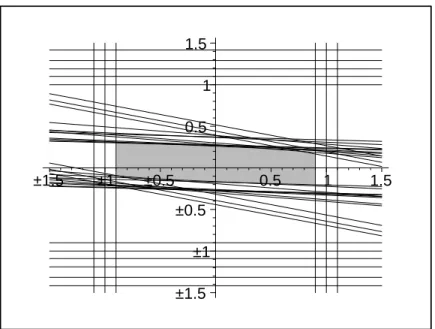
proposi-tion 1.4.4 insures that the set M of α-admissible observer initial states corresponding to the polyhedron P is nonempty and is entirely determined by proposition 1.4.1, and we have the following scheme:
–1.5 –1 –0.5 0.5 1 1.5 –1.5 –1 –0.5 0.5 1 1.5
Figure 1.1: The colored region gives the graphic representation of M the set of α-admissible observer initial states corresponding to the polyhedron P.
Remark 1.5.1 .
1) Like it was established in proposition 1.4.4, we notice that the triangle T P whose three vertices are v1, v2 and v3 is well inside the set of α-admissible observer initial
states corresponding to the polyhedron P.
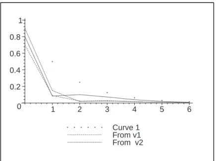
2) For z0 ∈ M, we know that the estimation error (1.10) verifies kei(x0)k ≤ αi,
∀i ≥ 0 from any initial state x0 ∈ P. By proposition 1.4.1, it is sufficient to verify it
for i = 0, ..., 4 and from vertices vj, j = 1, 2, 3 as initial states. To illustrate that, we
take z0 =
µ 0.8 −0.1
∈ M, and we represent the l∞ norm of the estimation errors
(1.10) which are plotted in Fig.1.2 from initial states v1, v2, v3, and their comparison
with curve 1 representing αi, i ≥ 0.
3) If z0 6∈ M, we cannot know starting from which rank i0 one will have kei(x0)k ≤
αi , ∀i ≥ i0 from some initial state x0 ∈ P. Fig.1.3 represents the estimation error
(1.10) from initial state v1 for z0 =
µ −1.5 0.5 ¶ (resp.z0 = µ 0 1 
) which are not in M, and their comparison with curve 1 representing αi, i ≥ 0. Note that i0 = 9(resp.
Curve 1 From v1 From v2 0 0.2 0.4 0.6 0.8 1 1 2 3 4 5 6
Figure 1.2: The simulation results for l∞ norm of the estimation error for z0 =
(0.8, −0.1) Curve 1 For zo = (–1.5 , 0.5) For zo = (0 , 1) 0 0.2 0.4 0.6 0.8 1 1.2 1.4 1.6 2 4 6 8 10 12 14
The parameters ei and αi being small from some row, their curves are almost stuck
to the x-axis, their pace are given in Fig.1.4 from i = 7.
Curve 1 For zo = (–1.5 , 0.5) For zo = (0 , 1) 0 0.002 0.004 0.006 0.008 8 9 10 11 12 13 14 Figure 1.4:
1.6
Discrete-time delayed system
In this section, we consider the discrete delayed system given by xi+1= N X j=0 Ajxi−j + Bui , i ≥ 0 xk ∈ Rn f or k ∈ {−N, −N + 1, ... , 0} (1.18)
the corresponding delayed output function is
yi = R
X
k=0
Ckxi−k , i ≥ 0 (1.19)
where xi ∈ Rn, ui ∈ Rm and yi ∈ Rq are, respectively, the state variable, the control
variable and the output variable, while Aj, B and Cj are constant matrices of respective
dimensions (n × n), (n × m), and (q × n). R and N are positive integers such that R ≤ N .
Without loss of generality, we assume that R = N, if not (R < N ) we can get Ck = 0
In the following, we suppose that the initial state (x−N, x−N +1, ..., x0) is unknown, then
we have to solve the states estimation problem of system (1.18) in basis of the output (1.19).
To solve this problem, we propose in the following to design an observer of the form zi+1= N X j=0 Fjzi−j+ P ui+ Dyi , i ≥ 0 zk∈ Rp f or k ∈ {−N, −N + 1, ... , 0} (1.20)
where zi ∈ Rp is the observer state, Fj, P and D are constant matrices of respective
dimensions (p × p), (p × m), and (p × q).
For ex0 = (x0, x−1, ..., x−N) an initial state of system (1.18), and T a matrix of suitable
dimension, let us introduce, for i ≥ 0, the vectors e
ei(ex0) = (ei(ex0), ei−1(ex0), ..., ei−N(ex0))T ∈ R(N +1)p
where
ei(ex0) = zi− T xi (1.21)
is the estimation error from the initial state ex0, and consider the new matrix eF of
dimension (N + 1)p × (N + 1)p defined by e F = F0 F1 · · · FN Ip 0p · · · · 0p 0p . .. ... ... ... ... ... ... ... 0p · · · 0p Ip 0p
where Ip and 0p are respectively the identity and the zero matrices of order p.
In order to lighten the notations, and when there is no confusion , we will denote eei(ex0)
by eei and ei(ex0) by ei.
The following propositions give sufficient conditions for the existence of an observer.
Proposition 1.6.1 For T ∈ L(Rn, Rp), the equation (1.20) specifies an observer of
the system (1.18, 1.19) if the following hold
1. FjT − T Aj = −DCj , f or 0 ≤ j ≤ N
2. P = TB
3. The matrix eF is stable.
Proof
Using (1.18, 1.19) and (1.20) yield ei+1 = zi+1− T xi+1
= N X j=0 Fjzi−j + D N X j=0 Cjxi−j + P ui − N X j=0 T Ajxi−j − T Bui = N X j=0 Fjei−j + N X j=0
(FjT + DCj− T A)xi−j + (P − T B)ui
.
If the conditions (1) and (2) hold then the observer error becomes
ei+1= N X j=0 Fjei−j (1.22) which is is equivalent to e ei+1= eF eei hence e ei+1 = eFiee0 . Thus
zi is an asymptotic state estimator of T xi ⇔ lim
j→+∞(zi− T xi) = 0 ⇔ lim i→+∞ei = 0 ⇔ lim i→+∞eei = 0 ⇔ T he matrix eF is stable . ¥
Proposition 1.6.2 For T ∈ L(Rn, Rp), the equation (1.20) specifies an observer of
the system (1.18, 1.19) if the following hold
1. FjT − T Aj = −DCj , f or 0 ≤ j ≤ N 2. P = TB 3. N X j=0 kFjk < 1. Proof
It is established in ([40]) that the condition (3) is sufficient to insure the stability of e
F , then we use proposition 1.6.1 to conclude.
Under the conditions of proposition 6.1 and given eP a convex and compact polyhedron of R(N +1)ncontaining the unknown initial state ex
0 = (x0, x−1, ..., x−N) of system (1.18),
we are interested to determine all observer initial state conditions ez0 = (z0, z−1, ..., z−N)
of system (1.20) such that the error (1.21) verifies
kei(ex)k ≤ αi ∀ i ≥ −N , ∀ex ∈ eP
where (αi)i≥−N is a positive decreasing sequence which verifies condition (1.11).
In other words, we aim to characterize the set fM of α-admissible initial states given by
f
M = {(z0, z−1, ..., z−N) ∈ R(N +1)p / kei(ex)k ≤ αi , ∀ i ≥ −N , ∀ex ∈ eP}.
Toward this end, let us define f
Mxe0 = {(z0, z−1, ..., z−N) ∈ R
(N +1)p / ke
i(ex0)k ≤ αi , ∀ i ≥ −N}
and eT the matrix of dimension (N + 1)p × (N + 1)n
e T = T 0p×n · · · 0p×n 0p×n T . .. ... ... . .. . .. 0p×n 0p×n · · · 0p×n T
where 0p×n is and the p × n -zero matrix.
Thus the following proposition holds
Proposition 1.6.3 For ex0 = (x0, x−1, ..., x−N) ∈ R(N +1)n, we have
f Mex0 = {ez0 = (z0, z−1, ..., z−N) ∈ R (N +1)p/ k eFi(ez 0 − eT ex0)k ≤ βi ∀ i ≥ 0} where βi = αi−N, i ≥ 0. Proof
For i ≥ 0, let us define the vectors e xi = (xi, xi−1, ..., xi−N) e zi = (zi, zi−1, ..., zi−N) then we have e ei = ezi− eT exi .
From proposition 6.1, it follows that e
ei = eFiee0
= eFi(ez
0 − eT ex0)
If ez0 ∈ fMex0 then
keik ≤ αi ∀ i ≥ −N
or
keik ≤ αi , kei−1k ≤ αi−1, ... , kei−Nk ≤ αi−N ∀ i ≥ −N
since
keeik = max(keik , ... , kei−Nk)
we deduce
keeik ≤ max(kαik , ... , kαi−Nk) = αi−N
i.e,
keeik ≤ βi , ∀ i ≥ 0.
Conversely if ez0 ∈ R(N +1)p is such that keeik ≤ αi−N , ∀ i ≥ 0
then
keik ≤ keei+Nk ≤ αi , ∀ i ≥ −N .
Hence ez0 ∈ fMxe0.
¥ From proposition 1.6.3, it follows that fMxe0 is of the same form as the set Mx0 defined
by (1.12), so fMxe0 can be expressed as in (1.14) f Mex0 = eS + eT ex0 where e S = {ξ ∈ R(N +1)p/ k eFiξk ≤ β i , ∀i ≥ 0}.
Therefore, it is obvious that theorem 1.3.2 gives sufficient conditions to characterize the set eS by a finite number of inequalities, and the results on the characterization of the set of α-admissible observer initial states of section 4 can be translated to the set fM. In the following proposition, we give other sufficient conditions to characterize the set fMxe0 by a finite number of inequalities
Proposition 1.6.4 Suppose that
N X j=0 kFjk2 ≤ α2 N +1 N X i=0 α2 i then f Mxe0 = {(z0, z−1, ..., z−N) ∈ R (N +1)p / ke ik ≤ αi ∀ i ∈ {−N, ..., 0, ..., N }}
The following lemma will help us to prove proposition 1.6.4.
Lemma 1.6.1 Suppose that k N X j=0 Fjzjk ≤ αN +1 , ∀ zj ∈ B(0, αN −j) Then f Mxe0 = {(z0, z−1, ..., z−N) ∈ R (N +1)p / ke ik ≤ αi ∀ i ∈ {−N, ..., 0, ..., N }}
where N is the number of delays in the state variable of system (1.18). Proof
From relation (1.22) , we have
ei = N X j=0 Fjei−j−1 , ∀ i ≥ N − 1 If ez0 ∈ fMNxe0 = {(z0, z−1, ..., z−N) ∈ R (N +1)p / ke ik ≤ αi ∀ i ∈ {−N, ..., 0, ..., N }} ,
from the hypothesis of lemma 1.6.1, we have
keN +1k = k N X j=0 FjeN −jk ≤ αN +1 then e z0 ∈ fMN +1ex0 = {(z0, z−1, ..., z−N) ∈ R(N +1)p / keik ≤ αi ∀ i ∈ {−N, ..., 0, ..., N, N +1}} therefore f MNex0 ⊂ fMN +1xe0 we deduce from propositions 1.3.2 and 1.3.3 that
f
MxNe0 = fMxN +1e0 = fMex0 .
¥ Proof of proposition 1.6.4
zj ∈ B(0, αN −j), we have k N X j=0 Fjzjk ≤ αN +1 ≤ ( N X j=0 kFjk2) 1 2 ( N X j=0 kzjk2) 1 2 ≤ ( N X j=0 kFjk2) 1 2( N X j=0 α2 N −j) 1 2 ≤ ( N X j=0 kFjk2) 1 2( N X j=0 α2 i) 1 2 ≤ αN +1. ¥
1.7
Conclusion
In this paper, we are interested to estimate a discrete system state, we suppose that the initial state is unknown but localized in a convex and compact polyhedron. We determine, under certain hypothesis, a class M such that the Luenberger observer (zi)i≥0 initialized with z0 ∈ M allows to realize the performance
kzi− T xik ≤ αi ; ∀i ≥ 0
where α = (αi)i is a predefined mode of convergence. After giving a theoretical and
algorithmic characterization of the set M, we showed that the used approach is easily extended to discrete delayed systems .
As a natural continuation of this work and inspired by what was done in [33], [34], we investigate the same problem in the presence of perturbations. It will be also interesting to study the continuous case.
[1] A. Alessandri and P. Coletta, Switching observers for continuous-time and discrete-time linear systems, In Proc. 2001 Amer. Control. Conf., Arlington, VA, June (2001).
[2] A. V. Balakrishnan, Applied Functional Analysis, Berlin, Springer-Verlag, (1976).
[3] A. Bensoussan and M. Viot, Optimal control of stochastic linear distributed pa-rameter systems, SIAM J. Control, 13 (1975), 904-926.
[4] B. E. Bona, Designing observers for time-varying state systems, in Rec. 4th Asilo-mar Conf. Circuits and Systems, (1970).
[5] M. Boutayeb and M. Darouach, Observers for linear time-varying systems, In Pro-ceedings of the 39th IEEE Conference on Decision and Control, Sydney, Australia, December (2000), 3183-3187.
[6] L. Chen and G. Bastin : On the model identifiability of stirred tank reactors, Proceedings of the 1st European Control Conference, 1 (1991), 242-247.
[7] R. F. Curtain and H. J. Zwart, An introduction to infinite-dimensional linear systems theory, Texts in applied mathematics, 21 (TAM 21), Springer Verlag, (1995).
[8] F.Esfandiari and H.K.Khalil, Output feedback stabilization of fully linearizable systems, Int. J.Control, 56 (1992), 1007-1037.
[9] M. Fliess and H. Sira Ramirez, Control via state estimations of some nonlinear systems, Proc. Symp. Nonlinear Control Systems NOLCOS (2004), Stuttgart, (accessible sur http://hal.inria.fr/inria-00001096).
[10] B.A. Francis, A Course in H∞-Optimal Control Theory, New York,
Springer-Verlag, (1987).
[11] J. P. Gauthier, H. Hammouri and S. Othman, A Simple Observer for Nonlinear Systems- Applications to bioreactors, IEEE Trans. on Auto. Control, 37 (1992), 6, 875-880.
[12] A.M. Gibon-Fargeot, H. Hammouri and F. Celle, Nonlinear observers for chemical reactor. Chem. Engng Sci. 49 (1994), 2287-2300.
[13] D. Gleason and D. Andrisani, Observer design for discrete systems with unknown exogenous inputs, IEEE Trans. Automat. Control, 35 (1990), 932-935.
[14] J.Han, A class of extended state observers for uncertain systems, Control and Decision, 10 (1995), N.1, 85-88 (In chinese).
[15] F.J.J.Hermans and M.B.Zarrop, Sliding-mode observers for robust sensor mon-itoring, Proceedings of 13th IFAC World Congress, SanFrancisco, USA, (1996),
211-216.
[16] A. Ichikawa, Optimal quadratic control and filtring for evolution equation with delays in control and observation, Control theory center, report 53, university of Warwick, coventry, (1978).
[17] J.A.Jackez, Compartmental analysis in Biology and Medicine, Amsterdam, (1972).
[18] E. W. Kamen, Block-form observers for linear time-varying discrete-time systems, In Proceedings of the 32nd IEEE Conference on Decision and Control, San Anto-nio,TX, December (1993), 355-356.
[19] J. C. Kantor, A finite dimensionnal nonlinear observer for an exothermic stirred-tank reactor, Chem. Engng Sci. 44 (1989), 1503-1510.
[20] DJ. Kazakos, SA. Manesis and TG. Pimenides : Nonlinear observers for fermen-tation processes and bioreactors. Proceedings of the 2nd European Control Con-ference. 1 (1993), 280-283.
[21] S.Kitamura and S.Nakagiri, Identifiability of spatially varying and constant param-eters in distributed systems of parabolic type, SIAM. J. Control and Optimization, vol. 15 (1977), N. 5.
[22] J.M.Legay, Introduction l’tude des modles compartiments, Informatique et Biosphre, Paris, (1973).
[23] J. L. Lions, Sur les sentinelles des systmes distribus, C.R.A.S. Paris, t.307, (1988).
[24] J. L. Lions, Furtivit et sentinelles pour les systmes distribus donnes incompltes, C.R.A.S. Paris, (1990).
[25] D.G.Luenberger, Observing the state of linear system, IEEE Trans. Mil. Electron., vol. MIL-8, Apr (1964), 74-80.
[26] D.G.Luenberger, Observers for multivariable systems, IEEE Trans. Automat. Contr., vol. AC-11 (1966), 190-197.