HAL Id: hal-02924040
https://hal-univ-tlse3.archives-ouvertes.fr/hal-02924040
Submitted on 27 Aug 2020
HAL is a multi-disciplinary open access
archive for the deposit and dissemination of
sci-entific research documents, whether they are
pub-lished or not. The documents may come from
teaching and research institutions in France or
abroad, or from public or private research centers.
L’archive ouverte pluridisciplinaire HAL, est
destinée au dépôt et à la diffusion de documents
scientifiques de niveau recherche, publiés ou non,
émanant des établissements d’enseignement et de
recherche français ou étrangers, des laboratoires
publics ou privés.
Machinery Fault Diagnostics Across Diverse Working
Conditions and Devices
Jian Zhou, Lian-Yu Zheng, Yiwei Wang, Christian Gogu
To cite this version:
Jian Zhou, Lian-Yu Zheng, Yiwei Wang, Christian Gogu. A Multistage Deep Transfer Learning
Method for Machinery Fault Diagnostics Across Diverse Working Conditions and Devices. IEEE
Access, IEEE, 2020, 8, pp.80879-80898. �10.1109/ACCESS.2020.2990739�. �hal-02924040�
A Multistage Deep Transfer Learning Method for
Machinery Fault Diagnostics Across Diverse
Working Conditions and Devices
JIAN ZHOU1, LIAN-YU ZHENG1, YIWEI WANG 1, AND CHRISTIAN GOGU2
1Department of Industrial and Manufacturing Systems Engineering, School of Mechanical Engineering and Automation, Beihang University, Beijing 100191,
China
2Institut Clément Ader CNRS/UPS/INSA/ISAE-SUPAERO/Mines Albi, Université de Toulouse, 31400 Toulouse, France
Corresponding author: Yiwei Wang ([email protected])
This work was supported in part by the National Natural Science Foundation of China under Grant 51805262, and in part by the Graduate Student Innovation Fund of Beihang University under Grant 010700-431054.
ABSTRACT Deep learning methods have promoted the vibration-based machinery fault diagnostics from manual feature extraction to an end-to-end solution in the past few years and exhibited great success on various diagnostics tasks. However, this success is based on the assumptions that sufficient labeled data are available, and that the training and testing data are from the same distribution, which is normally difficult to satisfy in practice. To overcome this issue, we propose a multistage deep convolutional transfer learning method (MSDCTL) aimed at transferring vibration-based fault diagnostics capabilities to new working conditions, experimental protocols and instrumented devices while avoiding the requirement for new labeled fault data. MSDCTL is constructed as a one-dimensional convolutional neural network (CNN) with double-input structure that accepts raw data from different domains as input. The features from different domains are automatically learned and a customized layer is designed to compute the distribution discrepancy of the features. This discrepancy is further minimized such that the features learned from different domains are domain-invariant. A multistage training strategy including pre-train and fine-tuning is proposed to transfer the weight of a pre-trained model to new diagnostics tasks, which drastically reduces the requirement on the amount of data in the new task. The proposed model is validated on three bearing fault datasets from three institutes, including one from our own. We designed nine transfer tasks covering fault diagnostics transfer across diverse working conditions and devices to test the effectiveness and robustness of our model. The results show high diagnostics accuracies on all the designed transfer tasks with strong robustness. Especially for transfer to new devices the improvement over state of the art is very significant.
INDEX TERMS Fault diagnostics, transfer learning, convolutional neural network, maximum mean differ-ence, multistage training.
I. INTRODUCTION
Bearings are the key rotating components in many mechan-ical systems. They are also the leading cause of failure in essential industrial equipment, such as induction motors, wheelset of railway bogie, aero-engines, wind-turbine power generation plants, steel mills, etc., where bearing faults account for 51% of all failures [1]. The failure of bear-ings may result in unwanted downtime, economic losses, and even human casualties. Therefore, the detection and The associate editor coordinating the review of this manuscript and approving it for publication was Huiling Chen .
diagnosis of rolling bearings are of major industrial signif-icance, consequently, the health assessment and fault diag-nostics of bearings in service received continuous attention from researchers [2].
The traditional bearing fault diagnostics normally includes two sequential steps of feature extraction and classifica-tion [1], [3]–[6]. However, extracting features manually (handcrafted features) suffers from problems such as highly dependency on the expertise, the requirement of complex signal processing techniques, the sensitivity to diagnostics tasks, etc. [7]. Lots of efforts have to be made to explore and design suitable features for different diagnostics task.
The introduction of deep learning (DL) methods into fault diagnostics has greatly improved the flexibility and gen-eralizability of diagnostic models [8], [9]. The hierarchi-cal structure of multiple neural layers of DL methods are capable of mining useful features from raw data layer by layer without any signal processing techniques [10]. This strong feature learning ability of the DL-based diagnostics models enables an end-to-end solution from raw signal to fault mode. In the past three years, the bearing fault diag-nostics based on DL methods achieved very high diagnosing accuracy [11]–[15].
However, these achievements are made under the assump-tions that a large amount of labeled fault data are available, and that the training and testing data are from the same distribution. These strong assumptions are typically difficult to satisfy in practice for the following reasons. Firstly, it is expensive to capture fault data and label them. Machines normally undergo a long degradation process from healthy to failure and the failure data occupy only a small proportion compared to the long healthy operating stage [16]. Even if the massive fault data can be monitored and accumulated, the fault labels are difficult to obtain as it is impractical to frequently shut down the machines to label the data. Secondly, the changing working conditions or the changing devices result in the difficulty of guaranteeing the training and testing data being from the same distribution. The working condition of a machine such as the rotating speed and the load may change during their service. It is unrealistic to build diagnostics models covering all potential working conditions. Even under constant speed and load, the data distribution is difficult to keep consistent since the vibration of the casing, the shaft and the environment noise may also affect the working condition to some extent. Furthermore, in practice, there are situations such that the diagnostics model trained by the data acquired from one device needs to be used for diagnosing the fault modes of another. For example, for a new machine with few faults data, it is highly desirable to transfer the diagnostics model trained on rich supervised information collected from other similar machines to this new target machine.
The aforementioned problems greatly impede the practical deployment of fault diagnostics models in industry, and thus indicate the urgency of developing new fault diagnostics models, which are able to be trained with unlabeled data and to transfer the diagnostics capability among diverse data distribution caused by multiple working condition or differ-ent devices. Extracting features from unlabeled data is an important direction [17]. Transfer learning [18], by releasing the constrain that training data must be independent and identical distributed with testing data, provides a promising idea to address the previous problems and has the potential to become state-of-the-art in the fault diagnostics area. Transfer learning, dealing with two datasets having different distribu-tions referred to as source domain and target domain, aims at solving a diagnostics problem with unlabeled and insufficient data in the target domain by utilizing the data in the source
domain [19]. Transfer learning can be roughly classified into non-deep transfer and deep transfer, depending on whether the deep learning method is used. For the former, to our best knowledge, [20] was the earliest research using transfer learning for bearing fault diagnostics, in which, singular value decomposition was used to manually extract features from vibration signals and transfer learning was used for classifica-tion. Transfer component analysis (TCA), as one of the repre-sentative methods of non-deep transfer, aims to learn a set of common transfer components underlying both domains such that when the raw data of the two domains are projected onto this subspace, the distribution difference of the two domains is greatly reduced [21]. Then the diagnostics model trained by the mapped source domain data can be used to diagnose the target domain data since they have very similar distribution. Ma et al. [22] proposed a weighted TCA method for bearing fault diagnostics that reduced both marginal and conditional distributions between different domains, improving the capa-bility of domain adaption. Similar, Qian et al. [23] proposed an improved joint distribution adaption (IJDA) method to align both the marginal and conditional distributions of dif-ferent datasets, which achieved good performance for transfer tasks under variable working conditions.
In contrast, deep transfer learning, aiming at transfer knowledge effectively by a deep neural network such as a convolutional neural network (CNN) or autoencoder (AE), adds constraints during deep model training process such that the features extracted from the source and target domains are domain invariant, i.e., features of the same type of fault learned from different domains are similar or even identi-cal. Compared to non-deep transfer, deep transfer fully uti-lizes the strong feature learning ability of deep learning and hence has large potential for further development. Therefore, the deep transfer learning framework is adopted in this paper. Li et al. [24] developed a deep distance metric learning method based on CNN that was able to significantly improve the robustness of fault diagnostics model against noise and variation of working conditions. Han et al. [25], [26] and Zhang et al. [27] proposed transfer learning frameworks based on pre-trained CNN, in which a CNN was firstly pre-trained on source domain and then the pre-trained CNN was transferred to target domain with proper fine-tuning based on domain adaptation theory. Xiao et al. [28] presented a novel fault diagnostics framework for the small amount of target data based on transfer learning and particularly increased the weights of the misclassified samples in training model by using a modified TrAdaBoost algorithm and con-volutional neural networks. Wen et al. [29] proposed a new method for fault diagnostics, which used a three-layer sparse auto-encoder to extract the features of raw data and applied the maximum mean discrepancy (MMD) term to minimizing the discrepancy penalty between the features from training data and testing data. Similar work based on deep transfer learning can also be found in [30]–[33].
The above research mainly addresses the transfer task in terms of diverse working conditions, fault severity and fault
types, in which cases the data distribution among diverse domains is different but relatively close. In practice, it is urgent and more challenging to address the transfer tasks across ‘‘different devices’’. Some researchers have begun to explore this issue. Li et al. [34] designed a deep transfer learning based on CNN, where the diagnostics ability trained on sufficient supervised data of different rotating machines is transferred to target equipment with domain adversarial training. Guo et al. [35] developed a deep convolutional transfer learning network consisting of two modules of con-dition recognition and domain adaption. The network was trained with unlabeled target domain data and achieved an accuracy around 86% when dealing with transfer tasks across the bearings from three different devices. Yang et al. [36] proposed a feature-based transfer neural network that iden-tified the health states of locomotive bearings in a real-case with the help of fault information from laboratory bearings, and obtained an average accuracy 81.15% over three designed transfer tasks. From the above-mentioned studies, it is clear that there is still large room for improvement of deep transfer learning methods in the context of diagnostics, in particular by improving the final accuracy of such approach (which is currently around 80%) to make it closer to 100%.
Motivated by the practical demand of the industry and the potential for improving the diagnostic accuracy for the ‘‘different devices’’ problem, inspired by the concept of trans-fer learning, we propose a multistage deep convolutional transfer learning framework (MSDCTL), which achieves the tasks of transfer fault diagnostics across multiple work-ing conditions as well as different devices with high diag-nostic accuracy, nearly 100%. MSDCTL is a double-input deep convolutional neural network structure that accepts raw data from the source domain and target domain as input. MSDCTL consists of a feature extraction module composed of four convolution-pooling blocks and a classification mod-ule composed of one flatten layer and two fully connected layers. Additionally, a customized layer is designed to com-pute the MMD to measure the difference of data distribution between the source and target domains. This difference is reduced during network training.
The main contributions of the paper are summarized below. We propose the MSDCTL (multistage deep convolutional transfer learning) framework to address the transfer tasks of bearing fault diagnostics across different working conditions and devices with high diagnostics accuracy. The network is trained with multiple stages of pre-training and fine-tuning, depending on the fault diagnostics tasks that are encoun-tered. Facing different tasks, the method is able to adaptively and flexibly complete the transfer learning task in multiple stages. The network accepts one-dimensional raw vibration signals as input. Therefore, no signal processing based fea-ture extraction or 2D image transformation [37]–[40] are required, providing an end-to-end solution for fault diagnos-tics. The ability of transfer learning from source domain to weakly supervised or even unsupervised target domain is also investigated.
The rest of the paper is arranged as follows. Section 2 intro-duces multi-input model structure and the principle knowl-edge of maximum mean difference and Section 3 details the framework of the proposed model and transfer learning method. In section 4, the proposed method is verified in two types of experiments composed of three datasets, one type relative to transfer to new working conditions and the other type relative to transfer to new devices. Finally, conclusions and highlights of the paper are given in Section 5.
II. THEORETICAL BACKGROUND
MMD is a powerful tool to realize the transfer fault diag-nostics of rotating machinery. It was first proposed by Gretton et al. [41] to test whether two distributions p and q are different on the basis of samples drawn from each of them, by finding a mapping function f maximizing the difference of the mean value of them. f belongs to F , which is a set of smooth functions defined in the reproducing kernel Hilbert space (RKHS), denoted as H . Let Xsand Xtbe two random variables following the distribution p and q, i.e., Xs ∼ pand
Xt∼ q. MMD is defined as the difference between the mean function values on the two distributions, as given in (1), where ‘‘: =’’ means ‘‘define’’ and sup(·) is the supremum of the input aggregate. A large value of MMD implies p 6= q.
MMD[F, p, q] := sup
f ∈F
(EXs∼p[f (Xs)] − EXt∼q[f (Xt)]) (1)
In terms of transfer learning, MMD is used as a metric to measure the difference of source domain and target domain. Given ns samples from source domain data Ds := {xis}ni=s1, and ntsamples from target domain Dt := {xit}ni=t1, a biased empirical estimation of (1) is obtained by replacing the distri-bution expectations with empirical expectation computed on the samples, as given in (2), where ˆDdenotes the estimation of MMD. When ˆDis large, the source domain data and the target domain data are likely from two distributions with large discrepancy while a small ˆDimplies the distribution of source and target domain data are close.
ˆ D[F, Xs, Xt] = sup f ∈F (1 ns ns X i=1 f(xis) − 1 nt nt X i=1 f(xtj)) (2)
The value of MMD depends heavily on the given set of continuous functions F , which should be ‘‘rich’’ and ‘‘restrictive’’ enough such that it is possible to find an appro-priate function f . According to [41], the unit ball on the RKHS is used as the function set F . Since RHKS is a com-plete inner product space, the mapping can be represented by a dot product, shown as:
f(xis) =< f , φ(xis)>H (3)
whereφ represent a mapping function xis → H. The property applies only when xis is mapped to RKHS, and it turns the value of mapping function f (xis) into the dot product of func-tion f and independent variable xis, so that f can be pulled out and the maximum value is easier to be calculated. Then (2) is
further reduced: ˆ D[p, q] = sup f ∈F Ep[< f , φ(xs)>H] − Eq[< f , φ(xt)>H] =sup f ∈F < Ep[φ(xs)] − Eq[φ(xt)], f >H = ||µp−µq||H (4)
where µp are the simplified representation of Ep[φ(xs)].
Squaring the above equation, (5) is obtained as follows. ˆ
D2[p, q] = hµp−µq, µp−µqiH
= Ephφ(xs), φ(xs)iH
+Eqhφ(xt), φ(xt)iH−2Ep,qhφ(xs), φ(xt)iH (5)
By means of the kernel mean embedding of distribu-tions, RKHS is induced by the characteristic kernels such as Laplace kernels and Gaussian kernels, which means hφ(xs), φ(xt)iHcan be calculated by kernel function k(xs, xt).
Thus, the empirical estimation of MMD based on the kernel mean embedding is computed as:
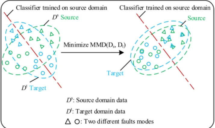
ˆ D2[Xs, Xt] = 1 n2 s ns X i=1 ns X j=1 k(xis, xjs) − 2 nsnt ns X i=1 nt X j=1 k(xis, xjt) +1 n2t nt X i=1 nt X j=1 k(xit, xjt) (6) After determining a kernel function, the value of MMD can be calculated and the distribution difference between two domains data can be quantified. In terms of transfer learning based on deep learning for fault diagnostics, MMD is typically used as the regularization term, serving as the constraint during the feature learning process. Optimization techniques are used to minimize the MMD computed on the features extracted from source domain and target domain such that the features from the two domains are becoming similar. By this way, the classifier that is trained on the source domain has therefore good performance of classifying fault modes from target domain, i.e., the diagnostics ability on source domain has transferred to target domain. Here it is assumed that fault label space of source domain and target domain are identical and the labeled source domain data and unlabeled target domain data are available during the feature learning process. Fig.1 shows the schematic diagram for a binary classification problem based on the idea of reducing distribution difference of source domain and target domain through minimizing MMD to improve the classification accu-racy on target domain data.
III. PROPOSED METHOD
A. DOUBLE-INPUT NETWORK STRUCTURE
Many neural networks are single-input-single-output. In order to compute the MMD, we design a double-input network structure shown in Fig.2, which accepts samples
FIGURE 1. Diagram of transfer learning by MMD minimization. It aims at reducing distribution difference and improving classification accuracy.
FIGURE 2. Flowchart of proposed double input model.
FIGURE 3. Architecture of proposed transfer learning model. C: convolutional layer, P: max-pooling layer, D: dropout layer, F: flatten layer, FC: fully connected layer.
from both source domain and target domain as input. The features are automatically learned and the MMD of the features are computed in the customized layer. The error between MMD and zero is back propagated to optimize the parameters of the model such that the difference of features from two domains are minimized.
B. ARCHITECTURE OF THE PROPOSED CNN MODEL
The structure of the proposed deep convolutional model is shown in Fig.3, which includes a feature extraction module consisting of four convolution-pooling blocks, and a classifi-cation module composed of one flatten layer and two fully connected layers. Dropout layers are added after the sec-ond and fourth convolution-pooling blocks to reduce risk of overfitting.
The input of the CNN are raw vibration data, i.e., accel-eration readings with a given sampling rate. In the convolu-tional layer, multiple filters are convolved with the input data and generate translation invariant features. In the subsequent pooling layer, the dimension of features is reduced by sliding a fixed-length window. The data flow from input layer to P1 layer is detailed below as an example to explain the convolution and pooling operation.
Let xIn = [x1, x2, . . . , xn] be the input of the network,
which is a segment of raw data with length n. Note that the superscript in the upper right corner represents the corre-sponding layer.βiis a one-dimensional filter with kernel size
h, i = 1,2,. . . , m. m is the number of filters. xC1denotes the output matrix of layer C1, which is a (n − h + 1)-by-m matrix. From xInto xC1, the convolution operation is carried out, which is defined by the dot product between filterβiand a concatenation vector xInk:k+h−1,
cj=ϕ(βi·xInk:k+h−1+b) (7) in which, · represents the dot product, b the bias term and ϕ the non-linear activation function. xIn
k:k+h−1 is a h-length vector xInk:k+h−1=[xk, xk+1, · · ·, xk+h−1], having the same shape with filter βi. As defined in (7), the output scalar cjcan be regarded as the activation of the filterβion
the corresponding concatenation vector xInk:k+h−1. By sliding the filterβiover xIn for k = 1 to k = n − h + 1, n − h + 1 scalar cj can be obtained, forming a column vector ci, also
known as a feature map:
ci=[c1, c2, . . . , cj, . . . , cn−h+1]T (8) One filter corresponds to one feature map. Since there are
m filters in the C1 layer, the output matrix xC1 after one convolutional layer is thus a (n−h+1)-by-m matrix. From the above operation it can be seen that one filter performs multi-ple convolution operations, during which the weights of the filter are shared. The feature map ci, obtained by convolving
one filterβiover the input data, represents the feature of the input data extracted from a certain level. By convolving the input data with multiple filters, a high-dimensional feature map containing multiple column vectors that reflect the input data from different perspectives are extracted.
xP1denotes the output matrix of the P1 layer, having the shape ((n − h + 1)/s, m), where s is the pooling length of P1 layer. From xC1to xP1, max pooling operation is carried out. Then the compressed column vector ci, which is denoted
as hi,is obtained by (9), where hl =max[c(l−1)s+1, c(l−1)s+2, . . . , cls].
hi=[h1, h2, . . . , hl, . . . , h(n−h+1)/s] (9)
After four blocks of convolution-pooling operation, a high-dimension feature map containing several column vectors is obtained by the feature extraction module. These column vec-tors represent features extracted from the input segment xIn from different perspectives and they should be concatenated to form a complete overview of xInsuch that the classification
module can ‘‘identify’’ it. To this end, the high-dimension feature map is flattened to a one-dimensional vector before being fed into the classification module.
Softmax function [42] is selected as the activation function of the last fully connected layer of the classification module, i.e., yout=softmax(xFC1·w + b), in which yOutis the output of softmax function, xFC1the input of the FC2 layer, w the weight matrix and b the bias vector of the FC2 layer. Softmax function gives a final score between 0 and 1, which can be roughly regarded as the probability of belonging to each label. Specifically, assuming a K -label classification task, the out-put of the softmax function yout = [yout1 , yout2 , . . . , youtK ] can be calculated as Eq.10, in which P(xFC1 ∈ i|wi, bi) denotes
the probability of xFC1 belonging to the i-th label given the corresponding weight and bias. The final output of the network is the health state label with the highest probability.
yout= yout1 ... youti youtK = 1 K P i=1 exp(wixFC1+bi) exp(w1xFC1+b1) ... exp(wixFC1+bi) exp(wKxFC1+bK) (10)
The weights of all convolutional layers and fully connected layers of the proposed model are initialized according to the uniform distribution w ∼ (−√6/(fi+ fo),
√
6/(fi+ fo)), where fi is the number of input units in the weight tensor, specifically, the kernel size for convolution layer and the size of input vector for fully connected layer. fois the number of output units, specifically, the number of filters for convolution layer and number of neurons for fully connected layer. The biases of each layer are initialized to 0.
C. OPTIMIZATION OBJECTIVES
During the process of model training, we set two optimization objectives and hence introduce two loss functions. The first is the categorical cross entropy L1, measuring the classification error. The second is mean absolute error (MAE) L2, which measures difference between MMD and zero label. The total loss function is L1when the model is single-input structure while it is L1+L2when the model is double-input structure.
Objective 1: Minimize the classification error on source domain
A high classification accuracy of CNN on the source domain data is the basis and prerequisite of the proposed transfer learning model. Therefore, the first objective is to minimize the classification error on the source domain. The categorical cross entropy loss function is employed. For a batch having N samples, the loss function L1 is defined as (11), where z is the ground truth and youti the softmax output. The subscript i denotes the i-th label out of K labels
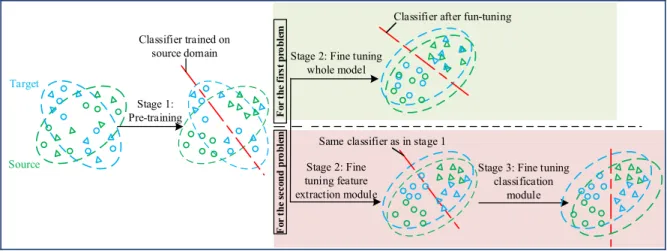
FIGURE 4. Flow chart of two-stage and three-stage transfer learning strategy.
and j denotes the j-th sample of the N -sample batch.
L1 = − 1 N N X j=1
[z(j)1 ln(yout,(j)1 )+, . . . , z(j)i ln(yout,(j)i )
+, . . . , +z(j) K ln(y out,(j) K )] = −1 N N X j=1 K X i=1 z(j)i ln(yout,(j)i ) (11)
Objective 2: Minimize MMD Between Features Extracted from Two Domains
The second objective is to reduce the distribution differ-ence of the features extracted from two domains during the model training. To this end, we create a customized layer, where the features extracted from the two domains are taken as input, and the output is the distribution difference of fea-tures of the two domains, i.e. the MMD. The loss function, i.e., MAE function, is defined as the absolute value of the difference between MMD and zero value (called zero label here). The features distribution discrepancy of two domains is reduced by minimizing the MAE function.
It should be pointed out that we take the features of the last fully connected layer as input of the customized layer for the following two considerations: 1) the gradient of the loss function will be back propagated from the last layer and the parameters of all layers will be adjusted. 2) the feature map of the last fully connected layer has a lower dimension compared with that of other layers, which can greatly reduce the calculation time of the customized layer.
Since RKHS is often a high dimensional or even infi-nite dimensional space, Gaussian kernel that can map to infinite dimensional space is selected as the corresponding kernel. For two observations in source domain xisand xjs, the Gaussian kernel is computed as (12), whereσ is the kernel bandwidth.
k(xis, xjs) = exp(−||xis− xjs||2/2σ2) (12)
By substituting (12) into (6) and specifying the number of samples with batch size N , the estimation of MMD is calculated by: ˆ D2[Xs, Xt] = 1 N(N − 1) N X i6=j exp(−||xis− xjs||2/2σ2) − 2 N2 N X i=1 N X j=1 exp(−||xis− xjt||2/2σ2) + 1 N(N − 1) N X i6=j exp(−||xit− xjt||2/2σ2) (13)
Mean absolute error (MAE) is calculated as (14). Since zero value label is set, the average absolute value of the mean difference between two domains data is directly taken as the mean absolute error.
L2= | ˆD2[Xs, Xt] − 0| = ˆD2[Xs, Xt] (14)
D. MULTISTAGE TRANSFER LEARNING STRATEGY FOR FAULT DIAGNOSTICS
In this section we elaborate on the multistage transfer learning strategy aiming to address the two types of fault diagnostics problems that are typically encountered by industry. The first is the transfer learning across various working condi-tions on the same device, where the distribution discrepancy between the source and target domains is normally small, while the second is the transfer learning across different devices, in which the distribution difference is considered large. The schematic diagram of the strategy is illustrated in Fig.4 and detailed as follows.
For the problem of multiple working condition, the train-ing strategy contains two stages: 1) pre-train whole network model with partial source domain data; 2) fine tune the whole network model with the rest source domain data and partial unlabeled target domain data. In the 1ststage, the network is set to single-input structure and trained as an ordinary CNN.
The loss function at this stage is L1, which is to measure the error between Os, i.e., the output of the CNN trained on the source domain, and Ls, i.e., the real label of source domain. In the 2nd stage, the model is adjusted to the double-input structure and the rest source domain data along with partial unlabeled target domain data are taken as the double input. The loss function at this stage is L1+L2. Optimization of L1 is to ensure that the high-accuracy diagnostics ability on the source domain data will not be affected when the network is fine-tuned, and the optimization of L2is to reduce the distribution difference of features extracted from two domains data. By optimizing L1+L2, the network retains high diagnostics accuracy on the source domain, and at the same time, the features extracted from the two domains tend to become similar (this process will be visualized by T-SNE in the case study). Due to the similarity of the features, the high-accuracy diagnostic capability of the network on the source domain data is transferred to the target domain data.
For the same device in the same health state, the raw monitoring data acquired under different working conditions are similar in nature. Therefore, by the fine tuning process in the 2nd stage, the features extracted from the same health state but under different working conditions can be easily clustered. In the 1ststage, the network has been well trained with the capability of recognizing different health states under one specific working condition, and the extracted features appear to be quite robust for being valid even when working conditions change. Since the network executes the classifica-tion based on these features, therefore, even after the working condition changed, the network can still recognize to which health state the feature belongs.
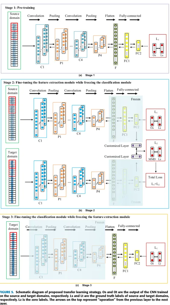
For the problem of different devices, the training strategy contains three stages: 1) pre-train the whole network model with partial source domain data as single input, as shown in Fig.5(a); 2) freeze the classification module and fine tune the feature extraction module with the rest of the source domain data and partial unlabeled target domain data as dou-ble input, shown in Fig.5(b); 3) freeze the feature extraction module and fine tune the classification module with very small amount of labeled target domain data as single input, shown in Fig.5(c). After stage 1, we obtained a pre-trained classifier with high accuracy on the source domain. Then the aim of stage 2 is to reduce the distribution discrepancy between the features of the two domains. By the end of stage 2, the feature extraction module has been well trained to cluster data of different labels in the target domain but the classification module still has the risk of misclassification. Therefore, in the stage 3, very small amount of labeled target domain data is used to fine tune the classification module so as to correspond the clustered data to correct label.
For different devices, even in the same health state, the monitoring data are very different in nature. Only fine tuning the feature extraction module in stage 2 may be insufficient to guarantee that the feature of each health state in the target domain can well match the feature of the same health state in the source domain (but indeed it well clustered the features
belong to different health state in the target domain). Since the network is trained on the source domain, it has the risk of misclassification on the target domain. To avoid this risk of the two-stage training strategy, we added the stage 3 that fine tunes the classification module with a very small amount of labeled target data.
The reasons for freeze operation are as follows. In stage 2, our purpose focuses on fine tuning the feature extraction module. During the fine-tuning process, the computation of the two loss functions (L1and L2) depends on the output of the classification module. If we do not freeze the classifi-cation module, the diagnostics results on the target domain will change with the fine-tuning process. This will result in the feature extraction module not being well trained. In the stage 3, we freeze the feature extraction module because it has been well-tuned in the stage 2. By this way, we can ‘‘freeze’’ its good ability of feature extraction.
The proposed strategy is based on the following consid-erations. Firstly, the labeled source domain data is normally sufficient but a large amount of labeled target domain is relatively difficult to obtain in practice. By directly training a network on the target domain from scratch it is hard to achieve a high accuracy due to insufficient data. Secondly, the source and target domains have different distributions but are related to each other. Therefore, using a network pre-trained on the source domain enables the network’s parameters to be easily recaptured in the target domain for feature and knowledge transfer [26]. In the field of object recognition, Oquab et al. designed deep CNNs based transfer learning method for the reuse of the parameters of the convolutional layers[43]. Yosinski et al. [44] investigated the transferability of fea-tures from source domain to target domain. Recently, studies regarding using pre-trained deep network based on transfer learning in the field of fault diagnostics also emerged [45]. In addition, separating the pre-training and fine-tuning is helpful to improve efficiency and flexibility of the transfer learning. One may want to finish the time-consuming net-work pre-training in advance and only fine-tune the netnet-work when dealing with new diagnostics task.
IV. CASE STUDY
A. DATASET DESCRIPTION
The following three datasets of bearing fault are employed in this case study: (1) Case Western Reserve University dataset (CWRU), (2) Intelligent Maintenance System dataset (IMS), and (3) the data collected from a self-developed test bench (HOUDE).
(1) The CWRU rolling bearing dataset is provided by the bearing data center of Case Western Reserve University [46]. The data are collected from 6202-SKF deeply grooved ball bearings in the experiments performed under four motor speed (1797, 1772, 1750 and 1730rpm) at a sampling fre-quency of 48 kHz. Four health conditions: outer race fault (OF), inner race fault (IF), roller element fault (RF) and nor-mal condition (NC) are introduced. For each fault type, single
FIGURE 5. Schematic diagram of proposed transfer learning strategy. Os and Ot are the output of the CNN trained on the source and target domains, respectively. Ls and Lt are the ground truth labels of source and target domains, respectively. Lz is the zero labels. The arrows on the top represent ‘‘operation’’ from the previous layer to the next layer.
FIGURE 6. Fault bearings after test: (a) IF, (b) RF (c) OF [48].
FIGURE 7. Schematic of HOUDE bearing fault test bench.
fault point with three severities levels, 0.007mil, 0.014mil, and 0.021mil are seeded, which is regarded as different cat-egories. Therefore, there are 10 health state labels in CWRU dataset, labeled as NC, RF(7), IF(7), OF(7), RF(14), IF(14), OF(14), RF(21), IF(21), OF(21).
(2) The IMS bearing data are from the Prognostics Center Excellence through the prognostic data repository contributed by Intelligent Maintenance System (IMS), Uni-versity of Cincinnati [47]. The experiments were run-to-fail tests under constant load. Four Rexnord ZA-2115 double row bearings were installed on one shaft that was driven by an AC motor at speed 2000 rpm. After run-to-fail test, IF, RF and OF occurred in three bearings, as shown in Fig.6. The bearing dataset we used in this paper is segmented from the run-to-fail data.
(3) The HOUDE dataset is acquired from a self-developed bearing fault test bench, shown in Fig.7. Five health condi-tions of 6308-NSK deeply grooved ball bearings are consid-ered, including the normal condition (NC) and four single fault, i.e., OF, IF, and RF and cage fault (CF), which are shown in Fig.8. The experiments were carried out at three motor speeds 1500rpm, 2000rpm and 2500rpm. The vibration data
FIGURE 8. Four fault modes of HOUDE bearings.
TABLE 1.Parameters of the proposed model. Parameters in the third column represents the a) Number of filters and kernel size in the convolutional layers, b) Pooling size in pooling layers, C) Percentage in dropout layers, and d) Number of neurons in fully connected layers.
were collected by an accelerometer mounted on the bearing house with a sampling rate of 20kHz.
B. COMPUTATION SETUP
The hyperparameters as well as the output shape of each layer of the CNN model detailed in Figure 3 are shown in Table 1. The number of neurons K of layer FC2 varies depending on the diagnostics tasks. It is worth pointing out that the sample length should be traded off between the number of samples and the feature information that one sample contains. A too-short length of time window may carry incomplete feature information, leading to the difficulty of diagnostics, while a long length of time window will result in insufficient training data. Based on the sampling rate of data used in this paper as well as other related research works, we take 1600 data points as one sample.
FIGURE 9. Confusion matrix of transfer learning task 1.2.
The value of parameters of the network could be a compli-cated problem. Based on our previous studies of using deep learning methods for fault diagnostics of rotating machin-ery, and based on the knowledge from the related literature, we found that changing the parameters of the network within a certain range will not have a great impact on the results. For example, we did the test that changed shape of the input, the number of filters and the kernel size to 2000-by-1,
40 and 260, respectively. We carried out the transfer tasks 1.1-1.6, which is detailed in Table 2. The test accuracies on the target domain of the six tasks are all over 99%.
The model is trained using the adaptive moment estima-tion (ADAM) solver. ADAM combines the Momentum and Root Mean Square Prop (RMSProp) optimization algorithms and develops independent adaptive learning rates for differ-ent parameters by calculating the first and second momdiffer-ent
FIGURE 10. Confusion matrix of transfer learning tasks 1.4-1.6.
estimates of gradient, due to which it often performs better with CNN than other alternative solvers.
The above network setting will be used in all the following cases. The network is developed based on the Keras frame-work.
C. TRANSFER LEARNING ACROSS MULTIPLE WORKING CONDITIONS
We first validate our model in the transfer tasks across mul-tiple working conditions of the same bearing. The transfer tasks are detailed in Table 2. We leave out the IMS data since it does not involve multiple working conditions. As detailed
in Section III, the training strategy of two stages is employed here. Each of source and target domain contains 3000 samples (reminder that the sample length is 1600). In the first stage of transfer learning, 1500 labeled samples of source domain data are used to pre-train the CNN model. Then 1500 unlabeled samples of the target domain data along with the remaining 1500 labeled samples of the source domain data are used to fine-tune the whole network in the second stage. Finally, the trained model is tested on the target domain.
The diagnostic accuracies tested on target samples are reported in Table 3. For comparison, the test accuracies given by the ordinary CNN without transfer learning (which is the
FIGURE 12. t-SNE figures of some layers during testing on the target domain of transfer learning task 1.5.
TABLE 2. Conditions and number of samples used for each transfer task.
pre-trained model in stage 1) are also listed. We implement each transfer task 10 times to assess the stability of the model and report the mean ± standard deviation. It can be seen that
for case 1.1 and 1.3, where the speed increment from source working condition to the target working condition is small (20rpm and 22rpm, respectively) and thus implies a small
FIGURE 13. Confusion matrix of transfer tasks 2.1-2.3.
difference between source and target domains, the accuracy of the ordinary CNN is fairly good but further improved nearly to 100% after transfer learning is integrated. For the remaining cases especially case 1.5, where the difference between the source and target domains is large due to the large speed increment, the ordinary CNN is almost not able to appropriately identify the fault modes. In contrast, after transfer learning is added, the performance is dramatically improved to nearly 100%. Note again here that one of the advantages of the proposed transfer learning framework is that it is does not need any labeled data in the target domain. Note that since for a new stage we used more source data to train the network, in order to eliminate any bias due to differ-ent amounts of training data, we also use all the 3000 source labeled samples to train the ordinary CNN and then test the trained network on the target domain. The results are listed in the last column of Table 3 for comparative study. We found
TABLE 3.Accuracy of each transfer task on the target domain.
that without transfer learning, even if more source labeled data are used, the classification accuracies tested on the target domain are not much improved accordingly. In some tasks such as task 1.5, the accuracies are even reduced. The reasons
FIGURE 14. t-SNE visualization of prediction result of task 2.1.
are analyzed as follows. Using more source domain data for training leads the network to better model the source data. If the target data and the source data have a relatively high similarity, then the test accuracies on the target domain will improve. For example, the speed increments in tasks 1.1, 1.3, and 1.4 are small, and thus the test accuracies are improved slightly. In contrast, if the target data and the source data have lower similarity, the accuracies on the target domain may reduce due to overfitting to the source domain (e.g., tasks 1.2, 1.5 and 1.6 where the speed increments are large).
The figures of confusion matrix corresponding to Table 3 are presented in Fig.9 (for CWRU dataset, only task 1.2 is given due to space limitation) and Fig.10 (for HOUDE dataset). Horizontal axis represents the predicted labels and the vertical axis is the true labels. Reminder that in cases 1.1-1.3, there are 10 health state labels while in cases 1.4-1.6 there are five labels.
To better illustrate the feature learning process of the CNN model, the t-distributed stochastic neighbor embedding (t-SNE) technique [49], which reduces the high
dimen-TABLE 4. Number of samples used for each transfer task between different devices.
TABLE 5. Accuracy of each stage for each transfer task.
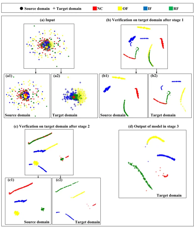
sional feature map to two dimensions, is employed to visualize the output of layers. We take the tasks 1.2 and 1.5 as examples, in which the improvement after trans-fer learning are most obvious. The symbols ‘‘·’’ and ‘‘+’’ denote the source samples and target samples, respec-tively, while the different colors represent the different fault label.
Fig.11 is the illustration of task 1.2. t-SNE figures of input layer, D1 layer, D2 layer and output layer during testing on the target domain are given in (a)-(d). In the input layer, the original data of source and target domains are scattered and overlapped densely. No obvious pattern or clusters can be observed. With data flowing through the feature extraction module and being processed by the convolution-pooling oper-ations, the data of the same color are gradually aggregated, as can be seen in Fig.11(c).
For comparison, we test the pre-trained CNN model on the target domain data and show the result in Fig.11(e). The result indicates that the source domain data have been well classified but there are considerable confusions between the labels RF(7), RF(14), OF(14), RF(21), and IF(21) in the target domain data. This is consistent with the result of the confusion matrix in Fig.9(a). By comparing the Figs. 11(e) and (d), the functions of the two stages are further clarified, i.e., stage 1 ensures a high accuracy on the source domain data and stage 2 transfer this ability to target domain data by reducing the discrepancy of the corresponding labels in the two domain.
The visualized result of task 1.5 is shown in Fig.12, where the t-SNE figures of input layer, D1 layer, D2 layer and output layer during testing on the target domain are given in (a)-(d). The test result on target domain given by the pre-trained CNN in stage 1 is also reported in (e), which shows that after stage 1, the source domain data have been well clustered, while in the target domain, NC is misclassified as RF and part of CF is confused with IF. About 30% target samples tested are misclassified after stage 1 but all correctly classified after stage 2, which is consistent with the confusion matrix in the Fig.10(c)-(d).
D. TRANSFER LEARNING BETWEEN BEARINGS IN DIFFERENT DEVICES
We further validate our model by the transfer tasks across dif-ferent devices, which is more challenging but practically very valuable. Three transfer tasks across the bearings of CWRU, IMS and HOUDE are considered, as reported in Table 4. In this case, CWRU data with 0.07mil fault size under speed 1730, HOUDE data under speed 1500 are used. Four health condition, OF, IF, RF and NC are considered. As detailed in Section III, the training strategy of three stages is employed here. Each of source and target domain contains 1200 samples. For each task, in the first stage, 600 samples are randomly drawn from the source domain to pre-train the model. In the second stage, the remaining 600 samples of the source domain as well as 600 unlabeled samples from the target domain are used to fine-tune the feature extraction module. In the third stage, a very small amount of labeled target samples (specifically, 12 labeled target samples of the remaining 600 target samples accounting for 1% of the total amount of the target samples) is used to fine-tune the classification module. After being trained, the model is tested with the 600 target samples.
For each task, the model was tested on the target domain every time a stage training is completed. The accuracy after each stage is presented in Table 5. We implement each transfer task 10 times to assess the stability of the model and report the mean ± standard deviation. For comparative study, the test accuracies of the ordinary CNN (i.e., in stage 1) trained with all the source domain data are also reported in the last column, similarly to what was done for the transfer learning investigation between different working conditions (Table 3 last column). The accuracies on the target domain do not accordingly improve even if more source data are used for training as shown in Table 5. These results are consistent with the fact that there are large differences in the data between the source and target domain when different devices are used, which do not allow proper classification when only source data is used, even if vast amounts of source data are available. The confusion matrix corresponding to Table 5 is shown
FIGURE 15. Confusion matrix of proposed model fine-tuned by unbalanced labeled target domain data in stage 3.
in Fig.13. In can be seen that for each task, the classification accuracies in the first and second stages are low but greatly improved after the third stage, reaching nearly 100%.
We take the transfer task 2.1 as an example to present the t-SNE visualization, as shown in Fig.14. Fig.14(b) is the result of validation on the target domain data using the pre-trained model obtained after stage1. It can be seen that the OF in the target domain are heavily confused with the RF in the source domain. The symbols ‘‘+’’ in red, blue and green are aggregated with the symbols ‘‘·’’ of blue, and the yellow ‘‘+’’ are aggregated with the green ‘‘·’’, implying that only the IF in target domain are classified correctly and about 75% of the testing data are misclassified. This is consistent with Fig.13(a) and the accuracy 23.67% in Table 5. Fig.14(c) presents the validation on the target domain after stage 2. All four labels of the target domain are confused with their counterparts in the source domain, which also agrees with Fig.13(b). The reason for the low classification accuracy is that in stage 2, the classification module is frozen during fine-tuning the feature extraction module, while this classification module was trained with source data in the previous stage thus has poor accuracy on the target data. It can be further noticed that the test samples in the target domain belonging to different labels are well clustered, meaning that the feature extraction module has been well trained in stage 2. Subse-quently, in stage 3, the classification module is fine-tuned using a very small amount of labeled target domain data while freezing the well-trained feature extraction module such that the classification module can achieve high accuracy. Indeed, we found that very small amount of labeled data (1/100 in case study) can greatly improve the classification accuracy of the model on the target domain data, as shown in Fig.13(c) and Fig.14(d).
TABLE 6.Accuracy and loss of proposed model fine-tuned by different amount of labelled target domain data.
TABLE 7.Accuracy of proposed model fine-tuned by unbalanced labelled target domain data.
It is worth noting that although large differences exist among the three bearing fault experiments, high trans-fer diagnostics accuracies were achieved with our pro-posed approach. Specifically, the faults in the bearings of HOUDE and CWRU were artificially introduced using electro-discharge machining while the IMS bearings under-went the run-to-fail tests and hence the IMS bearing faults were closer to reality, as can be seen from Fig.6 and Fig.8. In addition, the bearings are different in type, size, and man-ufacturer (Rexnord ZA-2115 for IMS, SKF6202 for CWRU, NSK6308 for HOUDE), which makes the transfer tasks more challenging. Despite this, the results of tasks 2.2 and 2.3 imply that even the diagnostics model trained using data collected from bearings with artificially seeded faults can have a good performance on bearing fault diagnostics tasks in real cases.
We notice that, indeed, a small amount of labeled target domain data is used to fine-tune the model when dealing with the transfer tasks across different devices. In practice, it is expected that the model should be able to achieve high accuracy while it uses as few as possible the labeled target domain data since labeled target data are difficult to obtain. Therefore, we design a few experiments to investigate at least how many labeled target domain data are required. The exper-iments are carried out on the transfer task 2.1. Reminder that the target domain data contains four types of fault and each fault type includes 150 samples. We gradually increase the amount of labeled target domain samples used for fine-tuning the classification module in stage 3, from four samples, which is a very extreme case, to 120 samples.
As can be seen from Table 6, the transfer learning model has low requirements for the amount of labeled target domain data: even if there are only four balanced labeled target sam-ples, the model still has an accuracy of 0.98.
TABLE 8. Comparison with related works for tasks across various working conditions.
TABLE 9. Comparison with related works for tasks across different devices.
We further explore the effect of unbalanced data on the accuracy of the proposed model. The following experiments are carried out on the transfer task 2.1. We remove one type of health state data from the target domain in the stage 3 of the training process. Then we test the trained network on the complete target domain, which includes four health state. The results are reported in Table 7 and the confusion matrix corresponding to Table 7 is shown in Fig.15. We found that indeed, the network recognized the three types of health states with high accuracy but fail to recognize the health state that it did not see in the fine tuning process.
Indeed, the issue of incomplete target data can bring some difficulties. While this issue is not to be underestimated, however, its severity is highly dependent on the application. For the applications of bearings, the faults are well known and documented. Therefore, it is quite easy to artificially introduce the various types of faults in order to obtain labeled fault data. For bearings diagnostics, incomplete data will probably be an issue that is easy to address, especially since only a very limited number of labeled data are required on new devices. For more general applications, the issue may be more severe and an important line of our future work will seek to alleviate it.
From the above case studies and discussions, the following conclusions can be drawn. For the fault diagnostics tasks that need to transfer across various working conditions, where the distribution discrepancy between the source and target domains is normally small, the two-stage transfer learning without the requirement of labeled target domain samples is enough to achieve good performance. For the diagnostics tasks that transfer across different devices, which is more challenging, the three-stages transfer learning strategy is required. Despite this, very few labeled target samples are enough to have a high classification accuracy of nearly 100%. Finally, we compare the proposed method with some related works that applied deep transfer learning on CWRU
dataset to study the variation of working conditions, and report the results in Table 8. The accuracies in the table are the average value over different transfer experiments carried out in the corresponding research work. All the research works show high diagnostics accuracies over 98%, with our model slightly higher than others. Note that one particularity of our model compared to the other ones cited in Table 8 is that it is able to work on the vibration signals directly without any preprocessing required such as Fast Fourier Transforma-tion. This provides an end-to-end solution for fault diagnos-tics, which reduces the dependencies on expertise and prior knowledge, and hence facilitates the use and deployment of diagnostics model. In addition, for the transfer tasks across devices, we compared with [35], [36], as given in Table 9. Similarly, the accuracies are the average value over different transfer experiments. All these works are end-to-end solu-tions using raw vibration data without any preprocessing as input.
V. CONCLUSION
The great success of deep learning methods in the field of fault diagnostics of rotating machinery in the past few years is based on the following two constraints, i.e., that sufficient labeled data are available and that the training and testing data are from the same distribution. However, these two constraints are typically difficult to satisfy in practice, and thus hinder the deep learning-based fault diagnostics methods being more widely employed in the industry. To release these constrains, we proposed a multi-stage deep convolutional transfer learning (MSDCTL) method. The main purpose is to achieve that the diagnostics model trained on one dataset (referred to as source domain) can be transferred to new diagnostics tasks (target domain). Two scenarios that are typically encountered in engineering are considered: trans-fer across diverse working conditions and across diftrans-ferent devices.
MSDCTL is constructed as a one-dimensional CNN con-sisting of a feature extraction module and a classification module. MSDCTL is with double-input structure that accepts raw data from different domains as input. The features from different domains are automatically learned and the dis-crepancy between domains is computed by maximum mean difference (MMD). This discrepancy is further minimized during network training such that the features from different domains are domain-invariant, by which way, the diagnos-tics ability on one dataset is transferred to new tasks with proper fine-tuning. A multistage training strategy including pre-training and fine-tuning is proposed to transfer the param-eters of the pre-trained model on source domain data to new diagnostics tasks instead of training a model from scratch, which reduces the requirement on the amount of data in the new task.
Three bearing fault datasets collected by three institutes, including one from our own, are used to verify the proposed method. The experimental protocols and the bearings used by the institutes are very different, which make the fault transfer diagnostics tasks more challenging. We designed nine transfer tasks covering different working conditions and devices to test the effectiveness and robustness of our method. The results show nearly 100% diagnostics accura-cies on all the designed tasks with strong robustness. The results demonstrate that when limited data of a target machine are available, it is feasible to acquire data from other sim-ilar machines and mining underlying shared features for diagnostics.
The limits of the current work are as follows. For transfer tasks across different devices, a small amount of balanced and complete labeled data from the target domain is still required. In our future work, we will focus on releasing this constraint. The study of transfer learning in fault diagnostics cases where the target data are incomplete or even unavailable will also be further studied.
REFERENCES
[1] M. M. M. Islam and J.-M. Kim, ‘‘Reliable multiple combined fault diagnosis of bearings using heterogeneous feature models and multi-class support vector machines,’’ Rel. Eng. Syst. Saf., vol. 184, pp. 55–66, Apr. 2019.
[2] J. Jiao, M. Zhao, J. Lin, and K. Liang, ‘‘Hierarchical discriminating sparse coding for weak fault feature extraction of rolling bearings,’’ Rel. Eng. Syst.
Saf., vol. 184, pp. 41–54, Apr. 2019.
[3] H. Feng, R. Chen, and Y. Wang, ‘‘Feature extraction for fault diag-nosis based on wavelet packet decomposition: An application on lin-ear rolling guide,’’ Adv. Mech. Eng., vol. 10, no. 8, Aug. 2018, Art. no. 168781401879636.
[4] Q. Zhang, J. Gao, H. Dong, and Y. Mao, ‘‘WPD and DE/BBO-RBFNN for solution of rolling bearing fault diagnosis,’’ Neurocomputing, vol. 312, pp. 27–33, Oct. 2018.
[5] L. S. Dhamande and M. B. Chaudhari, ‘‘Compound gear-bearing fault fea-ture extraction using statistical feafea-tures based on time-frequency method,’’
Measurement, vol. 125, pp. 63–77, Sep. 2018.
[6] C. Liu, G. Cheng, X. Chen, and Y. Pang, ‘‘Planetary gears feature extraction and fault diagnosis method based on VMD and CNN,’’ Sensors, vol. 18, no. 5, pp. 15–23, 2018.
[7] L. Jing, M. Zhao, P. Li, and X. Xu, ‘‘A convolutional neural network based feature learning and fault diagnosis method for the condition monitoring of gearbox,’’ Measurement, vol. 111, pp. 1–10, Dec. 2017.
[8] M. Hamadache, J. H. Jung, J. Park, and B. D. Youn, ‘‘A comprehen-sive review of artificial intelligence-based approaches for rolling element bearing PHM: Shallow and deep learning,’’ JMST Adv., vol. 1, nos. 1–2, pp. 125–151, Jun. 2019.
[9] R. Zhao, R. Yan, Z. Chen, K. Mao, P. Wang, and R. X. Gao, ‘‘Deep learning and its applications to machine health monitoring,’’ Mech. Syst. Signal
Process., vol. 115, pp. 213–237, Jan. 2019.
[10] H. Zhao, H. Liu, J. Xu, and W. Deng, ‘‘Performance prediction using high-order differential mathematical morphology gradient spectrum entropy and extreme learning machine,’’ IEEE Trans. Instrum. Meas., early access, Oct. 21, 2019, doi:10.1109/TIM.2019.2948414.
[11] S. Ma, W. Liu, W. Cai, Z. Shang, and G. Liu, ‘‘Lightweight deep residual CNN for fault diagnosis of rotating machinery based on depthwise separa-ble convolutions,’’ IEEE Access, vol. 7, pp. 57023–57036, May 2019. [12] M. He and D. He, ‘‘A new hybrid deep signal processing approach for
bearing fault diagnosis using vibration signals,’’ Neurocomputing, early access, Apr. 24, 2019, doi:10.1016/j.neucom.2018.12.088.
[13] D. Peng, Z. Liu, H. Wang, Y. Qin, and L. Jia, ‘‘A novel deeper one-dimensional CNN with residual learning for fault diagnosis of wheelset bearings in high-speed trains,’’ IEEE Access, vol. 7, pp. 10278–10293, Dec. 2019.
[14] M. He and D. He, ‘‘Deep learning based approach for bearing fault diagnosis,’’ IEEE Trans. Ind. Appl., vol. 53, no. 3, pp. 3057–3065, May 2017.
[15] X. Guo, L. Chen, and C. Shen, ‘‘Hierarchical adaptive deep convolution neural network and its application to bearing fault diagnosis,’’
Measure-ment, vol. 93, pp. 490–502, Nov. 2016.
[16] Y. Lei, N. Li, L. Guo, N. Li, T. Yan, and J. Lin, ‘‘Machinery health prognos-tics: A systematic review from data acquisition to RUL prediction,’’ Mech.
Syst. Signal Process., vol. 104, pp. 799–834, May 2018.
[17] H. Zhao, J. Zheng, W. Deng, and Y. Song, ‘‘Semi-supervised broad learning system based on manifold regularization and broad network,’’ IEEE Trans.
Circuits Syst. I, Reg. Papers, vol. 67, no. 3, pp. 983–994, Mar. 2020, doi:10. 1109/TCSI.2019.2959886.
[18] S. Jialin Pan and Q. Yang, ‘‘A survey on transfer learning,’’
IEEE Trans. Knowl. Data Eng., vol. 22, no. 10, pp. 1345–1359, Oct. 2010.
[19] R. Yan, F. Shen, C. Sun, and X. Chen, ‘‘Knowledge transfer for rotary machine fault diagnosis,’’ IEEE Sensors J., early access, Oct. 23, 2019, doi:10.1109/JSEN.2019.2949057.
[20] F. Shen, C. Chen, R. Yan, and R. X. Gao, ‘‘Bearing fault diagnosis based on SVD feature extraction and transfer learning classification,’’ in
Proc. Prognostics Syst. Health Manage. Conf. (PHM), Oct. 2015, pp. 1–6, doi:10.1109/PHM.2015.7380088.
[21] S. J. Pan, I. W. Tsang, J. T. Kwok, and Q. Yang, ‘‘Domain adaptation via transfer component analysis,’’ IEEE Trans. Neural Netw., vol. 22, no. 2, pp. 199–210, Feb. 2011.
[22] P. Ma, H. Zhang, W. Fan, and C. Wang, ‘‘A diagnosis framework based on domain adaptation for bearing fault diagnosis across diverse domains,’’ ISA
Trans., vol. 99, pp. 465–478, Apr. 2020, doi:10.1016/j.isatra.2019.08.040. [23] W. Qian, S. Li, P. Yi, and K. Zhang, ‘‘A novel transfer learning method for robust fault diagnosis of rotating machines under variable working conditions,’’ Measurement, vol. 138, pp. 514–525, May 2019.
[24] X. Li, W. Zhang, and Q. Ding, ‘‘A robust intelligent fault diagnosis method for rolling element bearings based on deep distance metric learning,’’
Neurocomputing, vol. 310, pp. 77–95, Oct. 2018.
[25] T. Han, C. Liu, W. Yang, and D. Jiang, ‘‘Learning transferable features in deep convolutional neural networks for diagnosing unseen machine conditions,’’ ISA Trans., vol. 93, pp. 341–353, Oct. 2019.
[26] T. Han, C. Liu, W. Yang, and D. Jiang, ‘‘Deep transfer network with joint distribution adaptation: A new intelligent fault diagnosis framework for industry application,’’ ISA Trans., vol. 97, pp. 269–281, Feb. 2020, doi:10.1016/j.isatra.2019.08.012.
[27] B. Zhang, W. Li, X.-L. Li, S.-K. Ng, ‘‘Intelligent fault diagnosis under varying working conditions based on domain adaptive convolutional neural networks,’’ IEEE Access, vol. 6, pp. 66367–66384, 2018.
[28] D. Xiao, Y. Huang, C. Qin, Z. Liu, Y. Li, and C. Liu, ‘‘Transfer learning with convolutional neural networks for small sample size problem in machinery fault diagnosis,’’ Proc. Inst. Mech. Eng., Part C, J. Mech. Eng.
Sci., vol. 233, no. 14, pp. 5131–5143, Jul. 2019.
[29] L. Wen, L. Gao, and X. Li, ‘‘A new deep transfer learning based on sparse auto-encoder for fault diagnosis,’’ IEEE Trans. Syst., Man, Cybern. Syst., vol. 49, no. 1, pp. 136–144, Jan. 2019.
![FIGURE 6. Fault bearings after test: (a) IF, (b) RF (c) OF [48].](https://thumb-eu.123doks.com/thumbv2/123doknet/12259900.320730/10.864.449.803.97.422/figure-fault-bearings-after-test-if-rf-of.webp)