Jacobi-like nonnegative joint diagonalization by congruence

HAL Id: hal-00921807

https://hal.archives-ouvertes.fr/hal-00921807

Submitted on 21 Dec 2013

HAL is a multi-disciplinary open access

archive for the deposit and dissemination of

sci-entific research documents, whether they are

pub-lished or not. The documents may come from

teaching and research institutions in France or

abroad, or from public or private research centers.

L’archive ouverte pluridisciplinaire HAL, est

destinée au dépôt et à la diffusion de documents

scientifiques de niveau recherche, publiés ou non,

émanant des établissements d’enseignement et de

recherche français ou étrangers, des laboratoires

publics ou privés.

Jacobi-like nonnegative joint diagonalization by

congruence

Lu Wang, Laurent Albera, Huazhong Shu, Lotfi Senhadji

To cite this version:

Lu Wang, Laurent Albera, Huazhong Shu, Lotfi Senhadji. Jacobi-like nonnegative joint diagonalization

by congruence. XXI European Signal Processing Conference (EUSIPCO’13), Sep 2013, Marrakech,

Morocco. 5 p. �hal-00921807�

JACOBI-LIKE NONNEGATIVE JOINT DIAGONALIZATION BY CONGRUENCE

Lu Wang

, Laurent Albera

, Hua Zhong Shu

, Lotfi Senhadji

1

_{INSERM, U 1099, 35042 Rennes Cedex, France}

2

_{LTSI, Université de Rennes 1, Campus de Beaulieu, 35042 Rennes Cedex, France}

_{LIST, Southeast University, 2 Sipailou, 210096, Nanjing, China}

4

_{Centre de Recherche en Information Biomédicale Sino-Français (CRIBs), Rennes, France}

_{INRIA, Centre Inria Rennes - Bretagne Atlantique, 35042 Rennes Cedex, France.}

Email: [email protected], {laurent.albera, lotfi.senhadji}@univ-rennes1.fr, [email protected]

ABSTRACT

A new joint diagonalization by congruence algorithm is pre-sented, which allows the computation of a nonnegative joint diagonalizer. The nonnegativity constraint is ensured by means of a square change of variable. Then we propose a Jacobi-like approach using LU matrix factorization, which consists of formulating a high-dimensional optimization problem into several sequential one-dimensional subprob-lems. Numerical experiments emphasize the advantages of the proposed method, especially in the presence of bottle-necks such as for low SNR values and a small number of available matrices. An illustration of blind source separation shows the interest of the proposed algorithm.

Index Terms— Nonnegative joint diagonalization by congruence, LU factorization, blind source separation, semi-nonnegative independent component analysis.

1. INTRODUCTION Consider a set C = {C(k)}K

k=1of K real symmetric matrices

sharing the following joint congruent structure:

C(k)= AD(k)AT ₍₁₎

where A ∈RN×Ndenotes an unknown transformation matrix, and D = {D(k)}K

k=1is a set of (N × N ) unknown diagonal

matrices. The Joint Diagonalization by Congruence (JDC) of such matrices consists of identifying the matrix A up to a di-agonal matrix and a permutation matrix. JDC is a fundamen-tal tool for Blind Source Separation (BSS) and Independent Component Analysis (ICA). In such problems, JDC identifies the mixing matrix A or its inverse from the observation vec-tor which obeys the linear instantaneous mixing model. The K matrices C(k) can be chosen as time-shifted covariance matrices, or higher order cumulant matrix slices.

The JDC problem has been mostly handled as a particular optimization problem. The algorithms computing A mainly depend on the criterion chosen to perform the optimization [1]. A great number of algorithms, such as JAD [2], FFDIAG

[3], LUJ1D [4] and J-DI [5], compute A by minimizing the following indirect least square criterion:

J (A) =PK

k=1k off(A

−1

C(k)A−T_)k2

F (2)

where off(.) nullifies the diagonal parts of the input matrix, the superscript−T_{means the inverse of the transposed matrix,}

and k.kF denotes the Frobenius norm. Other cost functions

are also used. ACDC [6] and the sub-spaces fitting algorithm [7] estimate A and the set D by using a direct least square criterion. Pham proposed an information theoretic criterion [8], which requires the target set C to be positive definite.

Recently BSS involving nonnegativity constraint has shown an interest in numerous applications such as image processing, data mining and biomedical engineering (see chapter 13 of [9]). Some BSS applications only involve a nonnegative mixing matrix A, such as magnetic resonance spectroscopy [10]. In this paper, we present a nonnegative JDC algorithm based on criterion (2), which is committed to seek a nonnegative joint diagonalizer A. The nonnegativity constraint is imposed by means of a square change of vari-able. Then a Jacobi-like approach based on LU matrix fac-torization is presented, which formulates a high-dimensional optimization problem into several sequential one-dimensional subproblems. Numerical experiments emphasize the advan-tages of the proposed method, especially in the presence of bottlenecks such as for low Signal to Noise Ratio (SNR) val-ues and a small number of matrices to be jointly diagonalized. An illustration of BSS of infrared spectra shows the interest of the proposed algorithm.

2. NONNEGATIVE JOINT DIAGONALIZATION A way of imposing nonnegativity of any matrix belonging to RN×N

+ is through a square change of variable:

A = B Bdef= B 2 (3) with B ∈ RN×N, as originally proposed in [11] for Non-negative Matrix Factorization (NMF), where stands for

Hadamard product. By assuming that A is non singular, the minimization of (2) such that A is nonnegative can be re-formulated as an unconstrained problem by minimizing the following criterion: J+(B) = K X k=1 k off((B 2)−1_C(k)_(B 2₎−T_)k2 F (4)

Minimizing (4) with respect to (w.r.t) B is the main goal of this paper. For this purpose, based on LU matrix factorization, the high dimensional optimization problem is then reduced to the search of a sequence of sparse triangular matrices. Hence we obtain a NonNegative extension of Afsari’s LUJ1D algo-rithm [4], namely NNLUJ1D. Let’s recall the following defi-nition:

Definition 1 A unit triangular matrix is a triangular matrix whose main diagonal elements are equal to1.

Then any non singular matrix B ∈RN×N can be factorized as B = LU ΛΠ, where L ∈ RN×N is a unit lower trian-gular matrix, U ∈RN×N is a unit upper triangular matrix, Λ ∈RN×N _{is a diagonal matrix and Π ∈R}N×N _{is a}

permuta-tion matrix. Consequently, due to the fact that (LU ΛΠ) 2= (LU ) 2_Λ 2_{Π and the indeterminacies of the JDC problem,}

the matrix B solving (4) can be chosen as B = LU without loss of generality. Now, let’s consider the following definition and lemma:

Definition 2 An elementary triangular matrix T(i,j)(a) is a unit triangular matrix whose non-diagonal elements are zeros except the(i, j)-th entry, which is equal to a.

Lemma 1 Any (N ×N ) unit lower (or upper) triangular ma-trix can be factorized as a product ofN (N −1)/2 elementary lower (or upper, respectively) triangular matrices.

The proof of lemma 1 is straightforward by reducing L (or U ) into identity matrices using Gaussian elimination. Lemma 1 yields that B can be written as a product of elementary triangular matrices: B = N Y j=1 N Y i=j+1 L(i,j)(`i,j) N Y i=1 N Y j=i+1 U(i,j)(ui,j) def = N(N−1) Y (i6=j) T(i,j)(ti,j) (5) where T(i,j)(ti,j) is defined for the sake of convenience as

follows: T(i,j)(ti,j) = ( L(i,j)(`i,j), if i > j U(i,j)(ui,j), if i < j (6)

and N(N − 1) is the total number of elementary lower and upper triangular matrices. As a consequence, the minimiza-tion of (4) is reduced to the sequential search of the N(N −1) parameters ti,j. Indeed, instead of simultaneously

identify-ing these N(N − 1) parameters, a Jacobi-like procedure will

repeat several sweeps of N(N − 1) sequential optimizations until convergence. Each optimization w.r.t only one parame-ter ti,j with a selected (i, j) index. Let ˜A and ˜B denote the

current estimate of A and B before estimating the parameter ti,j, respectively. Then ˜A(new)and ˜B(new)stand for ˜A and ˜B

updated by T(i,j)(ti,j), respectively.

Proposition 1 If we have ˜B(new)= ˜BT(i,j)(ti,j), then ˜A(new)=

( ˜B(new)₎ 2_{can be written as a function oft}

i,jas follows:

˜

A(new)= ( ˜B 2)T(i,j)(t2_i,j)+2 ti,j(˜bi ˜bj)ejT (7)

where ˜bi denotes thei-th column of ˜B, and ej is the j-th

column of the identity matrixI ∈RN×N.

The proof of proposition 1 is straightforward and therefore omitted. A natural way to compute the parameter ti,j is to

minimize the criterion (4) w.r.t ti,jby replacing matrix B by

˜

BT(i,j)(ti,j). We use J+(ti,j) instead of J+( ˜BT(i,j)(ti,j))

for the sake of convenience.

According to (4), the minimization of J+(ti,j) requires to

express the following update of the K matrices C(k): C(k,new)= ( ˜A(new))−1_C(k)_{( ˜A}(new)₎−T ₍₈₎

as an explicit function of ti,j. This can be done by means of

proposition 1. From equation (7), the first term of the sum is a non singular matrix and the second term is a rank-1 matrix. The sum of such two matrices can be inverted by Sherman-Morrison formula [12]:

Theorem 1 Suppose that R is a non singular square matrix andu, v are two vectors satisfying 1+vT_R−1

u 6= 0, then: (R + uvT₎−1 = R−1 −R −1 uvT_R−1 1 + vT_R−1_u (9)

Suppose that ˜B, and the two vectors 2 ti,j(˜bi ˜bj) and ej

satisfy the conditions of the Sherman-Morrison formula, the expression of ( ˜A(new)₎−1_{has the following form:}

( ˜A(new))−1_{= T}(i,j)_(−t2 i,j)Q( ˜B 2₎−1 (10) with: Q = I − 2ti,j 1 + 2ti,jβj βeiT (11)

where I ∈RN×N is the identity matrix, β = ( ˜B 2₎−1_(˜b

i ˜bj)

is a column vector and βj is the j-th element of β. Inserting

(10) into (8), C(k,new)can be rewritten by: C(k,new)= T(i,j)(−t2_i,j) Q ˜C(k)QT_T(i,j)_(−t2

i,j)

T ₍₁₂₎

where ˜C(k) = ˜A−1C(k)A˜−T _{is a constant matrix. Then}

through a straightforward computation of (12), each ele-ment of C(k,new) can be expressed as a function of ti,j as

Proposition 2 Each non-diagonal element of C(k,new) is a rational function inti,j:

C_m,n(k,new)= E(k,3)_m,nt3_i,j+ E_m,n(k,2)t2_i,j+ E_m,n(k,1)ti,j+ Em,n(k,0) (13)

whereEm,n(k,3),Em,n(k,2),Em,n(k,1)andEm,n(k,0) are the(m, n)-th

el-ements of the(N ×N ) symmetric coefficient matrices E(k,3), E(k,2),E(k,1) andE(k,0), respectively, with1 ≤ m 6= n ≤ N . These coefficients are defined as follows:

Em,n(k,3)=            2( ˜C_j,j(k)βm− ˜C (k) m,jβj) (1 + 2ti,jβj)2 if n = i, 1 ≤ m 6= i ≤ N En,m(k,3) if m = i, 1 ≤ n 6= i ≤ N 0 otherwise (14) Em,n(k,2)=                                  4( ˜C_j,j(k)βmβn+ ˜Cm,n(k)βj2−( ˜C (k) m,jβn+ ˜Cj,n(k)βm)βj) (1 + 2ti,jβj)2 if 1 ≤ m < n ≤ N, m 6= i, n 6= i 4( ˜Cj,j(k)βmβn+ ˜Cm,n(k)βj2−( ˜C (k) m,jβn+ ˜Cj,n(k)βm)βj)− ˜Cm,j(k) (1 + 2ti,jβj)2 if n = i, 1 ≤ m < i E(k,2)n,m if 1 ≤ n < m ≤ N 0 otherwise (15) Em,n(k,1)=            4 ˜Cm,n(k)βj−2( ˜Cm,j(k)βn+ ˜Cj,n(k)βm) (1 + 2ti,jβj)2 if 1 ≤ m < n ≤ N En,m(k,1) if 1 ≤ n < m ≤ N 0 otherwise (16) Em,n(k,0)=      ˜ Cm,n(k) (1 + 2ti,jβj)2 if 1 ≤ m 6= n ≤ N 0 otherwise (17)

where ˜Cm,n(k) is the(m, n)-th element of the matrix ˜C(k).

The proof of proposition 2 is omitted due to lack of space. Then the total sum of the squares of these non-diagonal ele-ments can be expressed in a compact matrix form as follows:

J+(ti,j) = K X k=1 kE(k)τ k2_F= τT_Q Eτ (18) with: Q_E =PK k=1E (k)T_E(k) ₍₁₉₎

where E(k)= [vecE(k,3), vecE(k,2), vecE(k,1), vecE(k,0)] is a (N2_{×4) matrix, τ = [t}3

i,j, t2i,j, ti,j, 1]Tis a 4-dimensional

pa-rameter vector, and vec(.) reshapes a matrix into a column vector. Matrix QEis a (4×4) symmetric coefficient matrix.

Equation (18) shows that J+(ti,j) is a rational function,

where the degrees of the numerator and the denominator are 6 and 4, respectively. The global minimum ti,j can be

ob-tained by computing the roots of its derivative and selecting the one yielding the smallest value of (18). Once the opti-mal ti,jis computed, the matrix ˜A is updated by computing

( ˜BT(i,j)(ti,j)) 2. Then the Jacobi-like procedure is repeated

to compute ti,j with the next (i, j) index. The processing of

all the N (N −1) parameters is called a sweep. The algorithm requires several sweeps to converge and can be stopped when the value of (18) falls below a fixed small positive threshold.

3. SIMULATION RESULTS

In this section, the performance of the proposed NNLUJ1D algorithm is evaluated with synthetic data, in order to show the influence of SNR and the number K of matrices to be jointly diagonalized. The proposed algorithm is compared with two classical non-orthogonal JDC methods, namely FF-DIAG [3] and LUJ1D [4]. Then an illustration of BSS appli-cation is given to show the interest of the proposed algorithm. The performance is measured in terms of the error between the true diagonalizer A and its estimate ˜A. So the scale and permutation invariant distance defined in [13] is used:

∆(A, ˜A) = min

Π Ψ(A, ˜AΠ) (20) where the distance (20) requires to sweep all the (N × N ) permutation matrices Π, and:

Ψ(M , ˜M ) = 1 N N X n=1 kmn− ˜ mnTmn ˜ mnTm˜n ˜ mnk2F (21)

with mn and ˜mn the n-th columns of M and ˜M ,

respec-tively. A small ∆(A, ˜A) value means a better JDC perfor-mance in the sense that ˜A is closer to A.

The synthetic matrix set C is generated randomly accord-ing to the JDC model (1). In the followaccord-ing tests, A ∈R3×3₊ is generated according to (3) where B ∈R3×3 _{is a random}

matrix with elements independently drawn from a real zero-mean unit-variance Gaussian distribution. The diagonal ele-ments of D(k)∈R3×3_{are similarly generated. The resulting}

target set CN is perturbed by a white Gaussian noise array N :

CN = C kCkF + σN N kN kF (22)

where σN is a scalar controlling the noise level. Then the

SNR is defined as SNR = −20 log10(σN). Moreover, we

re-peat all the experiments with 500 independent Monte Carlo trials. All the algorithms stop either when the relative error of the corresponding criterion between two successive sweeps is less than 10−5 or when the number of sweeps exceeds 500. All the algorithms are initialized by identity matrices.

3.1. Effect of SNR

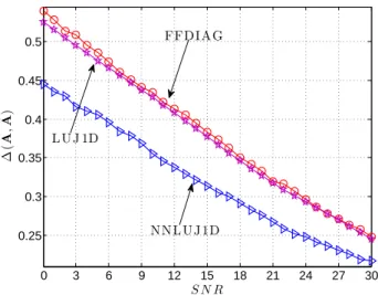
In this test, the compared algorithms are applied to noisy data for different SNR levels. The number of matrices is set to K = 3. We repeat the experiment with SNR rang-ing from 0 dB to 30 dB. Figure 1 shows the averaged er-ror ∆(A, ˜A) of compared algorithms as a function of SNR.

0 3 6 9 12 15 18 21 24 27 30 0.25 0.3 0.35 0.4 0.45 0.5 ∆ (A , ˜ A) S N R FFDIAG L UJ 1D NNL UJ 1D

Fig. 1. The average error ∆(A, ˜A) evolution of compared algorithms versus SNR. The dimension of A and the number of matrices are set to N = 3 and K = 3, respectively.

One can notice that, as SNR grows, the performance of all the JDC methods increases quasi-linearly. The difference be-tween FFDIAG and LUJ1D is small. It appears that the pro-posed NNLUJ1D algorithm achieves better estimations than FFDIAG and LUJ1D, especially when the SNR values are lower than 15 dB.

3.2. Effect of the number of matrices

In this test, the effect of the number K of matrices on the performance of the compared algorithms is evaluated. The SNR value is fixed to 5 dB. We repeat the experiment with K ranging from 3 to 30. Figure 2 shows the averaged error ∆(A, ˜A) of compared algorithms as a function of K. For all the JDC algorithms, the increase of K induces better es-timation performance. The classical algorithms FFDIAG and LUJ1D behave similarly. NNLUJ1D maintains a competitive advantage over FFDIAG and LUJ1D through all K values.

3.3. Performance of BSS of infrared spectra

In this section, we demonstrate the potential usefulness of the proposed algorithm through a BSS application carried out on infrared spectra. NNLUJ1D is compared with three well-known BSS algorithms, namely the ICA methods CoM2 [14] and SOBI [15], and a NMF method based on alternating NonNegative Least Squares (NNLS) [16]. Three gas phase Fourier-transform infrared spectra of three materials, namely Toluene, Dichloromethane and Methanol (see figure 3(a)), with 0.125 cm−1 resolution [17], serve as source signals s. Three linear observations (see figure 3(b)) are created by the linear mixed model x = As with A similarly generated as in the previous section. The matrix set C contains 12 matrix slices chosen from the third and fourth order cumulants.

3 6 9 12 15 18 21 24 27 30 0.38 0.4 0.42 0.44 0.46 0.48 0.5 K ∆ (A , ˜ A) NNL UJ 1D L UJ 1D FFDIAG

Fig. 2. The average error ∆(A, ˜A) evolution of compared al-gorithms versus the number of matrices K. The dimension of A and the SNR are set to N = 3 and SNR = 5 dB, respectively. Table 1. Average estimating errors of the mixing matrix ∆(A, ˜A) and the sources ∆(sT_{, ˜s}T_{) of four methods for BSS}

of infrared spectra

NNLUJ1D CoM2 SOBI NNLS ∆(A, ˜A) 0.0401 0.0494 0.2845 0.1144 ∆(sT_{, ˜s}T_{) 0.0690 0.0837 0.4165 0.1863}

The average estimation errors ∆(A, ˜A) of the mixing ma-trices and that ∆(sT_{, ˜s}T_{) of the source spectra of the compared}

methods are shown in table 1. It can be seen that the proposed NNLUJ1D method gives the smallest estimating errors both for A and s. The estimated spectra of the compared methods are displayed in figures 3(c) to 3(f). It shows that the pro-posed NNLUJ1D algorithm gives a better result than classic methods. The results infer that when the source spectra are partially correlated, using only the independency or the non-negativity may not yield a perfect decomposition. In such a case, the complementary nonnegative information along with the independence could improve the separation result.

4. CONCLUSION

In this paper, we address the problem of nonnegative JDC. We exploit the elementary triangular parameterization of the Hadamard square root of the nonnegative joint diagonalizer. Thus we propose a Jacobi-like approach. In each Jacobi-like iteration, the optimization is formulated into the minimization of a rational function w.r.t only one parameter. Numerical ex-periments on simulated data spotlight the advantages of the proposed method in the presence of bottlenecks, such as for low SNR values and a small number of available matrices to be jointly diagonalized. Furthermore, the potential interest of the proposed algorithm is demonstrated through a BSS

exper-0 1 2.5 4 5.5 x 104 1

2 3

(a) Source spectra

0 1 2.5 4 5.5 x 104 1 2 3 (b) Observations 0 1 2.5 4 5.5 x 104 1 2 3 (c) Estimated by NNLUJ1D 0 1 2.5 4 5.5 x 104 1 2 3 (d) Estimated by CoM2 0 1 2.5 4 5.5 x 104 1 2 3

(e) Estimated by SOBI

0 1 2.5 4 5.5 x 104 1 2 3 (f) Estimated by NNLS

Fig. 3. Infrared source spectra, mixtures and estimated spec-tra by NNLUJ1D, CoM2, SOBI and NNLS.

imental context.

5. REFERENCES

[1] G. Chabriel and J. Barrère, “A direct algorithm for nonorthogonal approximate joint diagonalization,” IEEE Trans. Signal Process., vol. 60, no. 1, pp. 39–47, 2012.

[2] J. F. Cardoso and A. Souloumiac, “Jacobi angles for simultaneous diagonalization,” SIAM J. Matrix Anal. Appl., vol. 17, pp. 161–164, 1996.

[3] A. Ziehe, P. Laskov, G. Nolte, and K. R. Muller, “A fast algorithm for joint diagonalization with non-orthogonal transformations and its application to blind source sep-aration,” J. Mach. Learning Res., vol. 5, pp. 777–800, 2004.

[4] B. Afsari, “Simple LU and QR based non-orthogonal matrix joint diagonalization,” in ICA 2006, Springer LNCS series, 2006.

[5] A. Souloumiac, “Nonorthogonal joint diagonalization by combining Givens and hyperbolic rotations,” IEEE Trans. Signal Process., vol. 57, no. 6, pp. 2222–2231, 2009.

[6] A. Yeredor, “Non-orthogonal joint diagonalization in the least-squares sense with application in blind source separation,” IEEE Trans. Signal Process., vol. 50, no. 7, pp. 1545–1553, 2002.

[7] A. J. van der Veen, “Joint diagonalization via subspace fitting techniques,” in Proc. ICASSP ’01, 2001, vol. 5, pp. 2773–2776.

[8] D. T. Pham, “Joint approximate diagonalization of pos-itive definite hermitian matrices,” SIAM J. Matrix Anal. Appl., vol. 22, pp. 1837–1848, 2001.

[9] P. Comon and C. Jutten, Handbook of Blind Source Sep-aration: Independent Component Analysis and Applica-tions, Academic Press, 2010.

[10] P. Sajda, S. Du, T. R. Brown, R. Stoyanova, D. C. Shungu, X. L. Mao, and L. C. Parra, “Nonnegative ma-trix factorization for rapid recovery of constituent spec-tra in magnetic resonance chemical shift imaging of the brain,” IEEE Trans. Med. Imag., vol. 23, no. 12, pp. 1453–1465, 2004.

[11] M. Chu, F. Diele, R. Plemmons, and S. Ragni, “Op-timality computation and interpretation of non negative matrix factorizations,” Tech. Rep., Wake Forest Univer-sity, 2004.

[12] M. S. Bartlett, “An inverse matrix adjustment arising in discriminant analysis,” Annals of Mathematical Statis-tics, vol. 22, no. 1, pp. 107–111, 1951.

[13] P. Comon, X. Luciani, and A. L. F. de Almeida, “Ten-sor decompositions, alternating least squares and other tales,” J. Chemometr., vol. 23, pp. 393–405, 2009. [14] P. Comon, “Independent component analysis, a new

concept?,” Signal Process., vol. 36, no. 3, pp. 287–314, 1994.

[15] A. Belouchrani, K. Abed-Meraim, J. F. Cardoso, and E. Moulines, “A blind source separation technique using second-order statistics,” IEEE Trans. Signal Process., vol. 45, no. 2, pp. 434–444, 1997.

[16] H. Kim and H. Park, “Nonnegative matrix factoriza-tion based on alternating nonnegativity constrained least squares and active set method,” SIAM J. Matrix Anal. Appl., vol. 30, no. 2, pp. 713–730, 2008.

[17] P. M. Chu, F. R. Guenther, G. C. Rhoderick, and W. J. Lafferty, “The NIST quantitative infrared database,” J. Res. Natl. Inst. Stand. Technol, vol. 104, no. 59, pp. 59– 81, 1999.