Predicting Bus End-Trip Delays Using Different Machine Learning Algorithms to Model Planning Effectiveness

Predicting Bus End-Trip Delays Using Different Machine Learning Algorithms to Model Planning Effectiveness

VICTOR HANNOTHIAUX

Département de mathématiques et de génie industriel

Mémoire présenté en vue de l’obtention du diplôme de Maîtrise ès sciences appliquées Mathématiques appliquées

Juin 2019

c

Ce mémoire intitulé :

Predicting Bus End-Trip Delays Using Different Machine Learning Algorithms to Model Planning Effectiveness

présenté par Victor HANNOTHIAUX

en vue de l’obtention du diplôme de Maîtrise ès sciences appliquées a été dûment accepté par le jury d’examen constitué de :

Guy DESAULNIERS, Ph.D., président

Andrea LODI, Ph.D., membre et directeur de recherche

Louis-Martin ROUSSEAU, Ph.D., membre et codirecteur de recherche Charles FLEURENT, Ph.D., membre

DEDICATION

“Study the past if you would define the future.” . . . Confucius

ACKNOWLEDGEMENTS

I would like to thank my research director Professor Andrea Lodi and my co-director Professor Louis-Martin Rousseau for guiding me and for giving me their confidence throughout the project. They helped me to distinguish the essential aspects of the project, and they always made time for me when necessary.

Also, I would like to thank Charles Fleurent, Loïc Bodart, Catherine Bédard, David Johannès and Madjid Aoudia from Giro who gave me access to all the data I needed and their interest for the project during the numerous meetings. They were always quick to answer any of my interrogations.

I would like to thank the chair of "data science for real-time decision making" and its partners ; GERAD, IVADO and CIRRELT, and the people who work here and helps me a lot : Mehdi, Koladé and Khalid.

I would like to thank the department of Mathématiques Appliquées et Génie Industriel (MAGI) of Polytechnique Montreal.

I would like to thank Ludovic, Igor, Defeng, Antoine, Mike and all the other postdocs, Ph.D. students and masters from Polytechnique for their help during the project.

I would like to thank James Moran, my squash partner, who took the time to read my thesis and help me to correct it.

Finally, I would like to acknowledge my family and my friends for their support, and especially Vincent, Jordan, Morgane, and Valentine.

RÉSUMÉ

Le transport public existe presque partout dans le monde. Cela permet à toutes les personnes le désirant de se déplacer d’un endroit à un autre d’une ville de façon économique et écolo-gique. De plus, de plus en plus de données sont disponibles de nos jours grâce aux systèmes embarqués à l’intérieur des véhicules. Ces données pourraient être utilisées dans une optique de prévision des retards, qui permettraient par la suite de les anticiper. Ainsi la fiabilité des horaires serait améliorée et plus de gens seraient suceptibles d’employer ce mode de trans-port. Des travaux ont été réalisés afin de prédire les retards en utilisant différentes données, cependant aucune d’elle ne l’a fait dans l’idée d’intégrer ces prévisions dans les procédures de création de planification de trajet.

Au cours de ce mémoire, divers modèles de prédicition de retard pour les fins de trajet sont essayés. Il ne s’agit pas de prédire le retard exact, mais de classifier les retards des fins de trajet. Afin d’être utile aux planificateurs d’horaires, ces modèles n’utilisent que des données qui peuvent se trouver en amont de la planification. Les données exploitées pour les modèles sont des observations historiques de la ville de Montréal. Deux problèmes de classification sont abordés au cours de ce mémoire. Le premier est un modèle de classification binaire qui prédit si un bus va finir son trajet en retard ou à l’heure. Le second est un modèle qui prévoit dans quel créneau de retard le bus va finir son trajet. Pour chacun des problèmes, trois algorithmes de machine learning pour l’estimation des retards sont testés : réseau de neurones, forêt aléatoire et arbre stimulé par gradient. De plus, une régression logistique est également testée afin de comparer les résultats par rapport à une méthode plus standard. Les modèles sont optimisés selon différentes méthodes et sont comparés en terme de précision et de temps d’entraînement.

Les modèles sont par la suite entraînés sur une période et testés sur d’autres afin d’étudier la possibilité d’intégrer ces modèles dans le processus de création de lignes. Par la suite, les prédictions sont utilisées afin de créer des distributions de probabilité pour les différents crénaux de retard pour les fins de trajet des bus. Les différents algorithmes sont testés afin de distinguer ceux qui reproduisent au mieux la réalité.

Le projet conclut sur la possibilité d’utiliser les données de planning pour prédire le retard des fins de trajet des bus. Une classification sur plusieurs classes peut être améliorée en intégrant de l’apprentissage non supervisée afin de déterminer les classes de retard. Il est également possible d’entraîner un modèle sur des périodes passées afin de prédire sur de futures périodes, mais cette méthode doit être encore améliorée.

ABSTRACT

Public transportation services are provided in almost all the cities of the world. They allow people to move through the cities in an economical and eco-friendly way. The buses are one of the possible solutions for public transportation. Moreover buses are interesting to study because more data are available from onboard systems and can be used to optimize service quality.

Indeed, preventing delays could improve service reliability and thus make people more likely to use public transport instead of their cars, which are currently more comfortable and more reliable. The first step in this process would be to forecast the delays. A lot of factors are linked to delays: peak-hour traffic, weather or accidents, etc. Some studies were conducted to predict end trips delay using real-time input which does not allow improvement to schedule reliability because these data are not available during planning.

This research focuses on modeling end-trip arrival time for each bus trip based only on offline input available to public transport planner. The models do not intend to predict the exact delays, but rather to classify them. The delays used to train and test the models are historical observations from the city of Montreal in autumn 2017. Two different classification problems were treated. The first one estimates the probability for a trip to end on-time or late. The second one estimates the slot of delay. For each problem, three different machine learning models were built and optimized: random forest, gradient boosted tree and artificial neural network. Also, logistic regression was tested in order to compare the results. Several optimization methods were tried. The models are compared in term of accuracy, recall, f1 score and training time.

The data from another period (autumn 2016) were then added to the database, and the model tested on the aggregated database. The model accuracy remained constant after the addition of the new period. The models were then fit on a single period (autumn 2016) and tested on the other one (autumn 2017) in order to check the possibility to use the model to forecast future schedules. The prediction is then used to generate a probability distribution for the different trips to end late to assess service reliability. The probability distributions are then compared with reality by comparing the distance between them and the frequencies of delays for the different trips. Normal distribution was also tested and obtained better results than the machine learning models.

The project concluded that it is possible to model end trip delays using offline data. Multi-label classification can be improved by using unsupervised learning to determine classes.

There is also a potential of training the models on some periods in order to predict for future ones.

TABLE OF CONTENTS

DEDICATION . . . iii

ACKNOWLEDGEMENTS . . . iv

RÉSUMÉ . . . v

ABSTRACT . . . vi

TABLE OF CONTENTS . . . viii

LIST OF TABLES . . . xii

LIST OF FIGURES . . . xv

LIST OF SYMBOLS AND ACRONYMS . . . xvi

CHAPTER 1 INTRODUCTION . . . 1

1.1 Framework of the project . . . 1

1.1.1 Basic concepts and definitions . . . 1

1.1.2 Case study : the Montreal Bus network . . . 2

1.1.3 GIRO . . . 3

1.1.4 Machine Learning . . . 3

1.2 Problem . . . 4

1.3 Objectives . . . 4

1.4 Work overview . . . 5

CHAPTER 2 LITERATURE REVIEW . . . 6

2.1 Public transport planning . . . 6

2.1.1 Planning methodology . . . 6

2.1.2 Quality factor for planning . . . 7

2.2 Advanced Public Transportation Systems . . . 8

2.2.1 Automatic Passenger Count . . . 8

2.2.2 Automatic Vehicle Location . . . 8

2.2.3 Smart card . . . 9

2.3 Service reliability . . . 10

2.3.2 Improving service reliability . . . 10

2.3.3 Measuring service reliability . . . 11

2.3.4 Delay propagation and bus bunching . . . 11

2.4 Predicting Delay in Public transportation . . . 12

2.4.1 Models using percentile methods . . . 12

2.4.2 Models using historical data . . . 12

2.4.3 Models using statistics . . . 13

2.4.4 Models using Machine Learning . . . 14

2.4.5 Models using Kalman Filter . . . 15

2.4.6 Conclusion . . . 15

CHAPTER 3 DATA ANALYSIS . . . 16

3.1 Planning Data . . . 16

3.2 APTS Data . . . 18

3.2.1 Raw data . . . 18

3.2.2 Extracting trip info . . . 20

3.3 External information . . . 21

3.3.1 Stop info . . . 21

3.3.2 Driver change . . . 22

3.3.3 Mean Layover Prev . . . 23

3.3.4 Day of the week . . . 23

3.3.5 Creating the final database . . . 23

3.4 Preprocessing . . . 23

3.4.1 Missing data . . . 24

3.4.2 Database cleaning . . . 24

3.4.3 Remove the lines of less than 100 occurrences . . . 24

3.4.4 Conclusion of preprocessing . . . 25 3.5 Database Analysis . . . 26 3.5.1 Features Analysis . . . 26 3.5.2 Features Correlation . . . 31 3.5.3 Objectives Analysis . . . 32 3.6 Autumn 2016 database . . . 33 3.6.1 General description . . . 34

3.6.2 Comparison to the Autumn 2017 database . . . 34

3.7 Data Analysis conclusion . . . 34

4.1 General Overview . . . 35

4.1.1 Methodology . . . 35

4.1.2 Metrics . . . 37

4.1.3 Building the different algorithms . . . 39

4.2 Binary classification . . . 40

4.2.1 Feature Optimization . . . 41

4.2.2 Oversampling . . . 44

4.2.3 Dimensionality reduction . . . 46

4.2.4 Removing the first trips . . . 47

4.2.5 Models on one line . . . 47

4.2.6 Overfitting . . . 48

4.2.7 Comments on the results . . . 50

4.3 Multi-label classification . . . 51

4.3.1 First results . . . 52

4.3.2 Unsupervised for classes . . . 54

4.3.3 Multi-label classification with optimized classes . . . 55

4.3.4 Characterisation of the errors . . . 59

4.4 Binary model on several periods . . . 61

4.4.1 Problems linked to linking different databases . . . 61

4.4.2 Bilinear model with both database . . . 62

4.4.3 Fitting on 2016 to predict on 2017 . . . 62

4.4.4 Unsupervised analysis . . . 63

4.5 Conclusion . . . 65

CHAPTER 5 EVALUATION OF THE SCHEDULE RELIABILITY . . . 66

5.1 Method for assessing schedule reliability . . . 66

5.1.1 Methodology . . . 66

5.1.2 Comparing to probabilistic laws . . . 67

5.1.3 Metrics for comparing distribution . . . 67

5.2 Assessing the service reliability . . . 68

5.2.1 Presentation of the results . . . 68

5.2.2 Analysis on peak hour periods . . . 69

5.2.3 Explaination of the difference between the models . . . 70

5.3 Conclusion . . . 70

CHAPTER 6 CONCLUSION AND RECOMMENDATIONS . . . 72

6.2 Limitations . . . 73 6.3 Future Research . . . 74 REFERENCES . . . 75

LIST OF TABLES

Table 3.1 Synthesis of preprocessing . . . 25

Table 3.2 Synthesis of the features . . . 26

Table 3.3 Number of records Via . . . 29

Table 3.4 Number of records Direction . . . 30

Table 3.5 Number of records Driver change . . . 31

Table 3.6 Number of records by days . . . 31

Table 3.7 Number of records Late . . . 33

Table 3.8 Number of records Late by category . . . 33

Table 4.1 Scores of the different algorithms before optimization . . . 41

Table 4.2 Results with different categorical features removed . . . 41

Table 4.3 Results with different numerical features removed . . . 42

Table 4.4 Results with ’via’ and ’driver change’ features processed as numerical features . . . 42

Table 4.5 Time feature . . . 43

Table 4.6 Block Rank features . . . 43

Table 4.7 Block Rank features . . . 43

Table 4.8 Scores with all the features in numeric categories . . . 44

Table 4.9 Scores with all the features except Week-days . . . 44

Table 4.10 Scores with RF depending on the Over-sampling Method . . . 45

Table 4.11 Scores with ANN depending on the Over-sampling Methods . . . 45

Table 4.12 Scores with GBT depending the Over-sampling Methods . . . 45

Table 4.13 Scores with logistic regression depending on the Over-sampling Methods 45 Table 4.14 Scores with RF depending on the Dimensionality Reduction factor . . 46

Table 4.15 Scores with ANN depending on the Dimensionality Reduction factor . 46 Table 4.16 Scores with GBT depending on the Dimensionality Reduction factor . 46 Table 4.17 Scores with Logisitic regression depending on the Dimensionality Re-duction factor . . . 47

Table 4.18 Scores of the different models with the first trips removed . . . 47

Table 4.19 Scores of the different models on the line 51 . . . 48

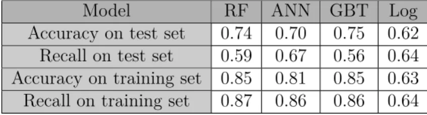
Table 4.20 Scores of the training and the test set for the different models . . . . 48

Table 4.21 Classification report for the Random forest algorithm . . . 52

Table 4.22 Classification report for the Gradient boosted tree algorithm . . . 52

Table 4.24 Classification report for the multi-linear logistic regression . . . 53

Table 4.25 Multi-label classification . . . 53

Table 4.26 Unsupervised clustering using k-means on Autumn 2017 . . . 54

Table 4.27 Classification report for the Random forest algorithm and 3 optimized classes . . . 55

Table 4.28 Classification report for the Random forest algorithm and 4 optimized classes . . . 55

Table 4.29 Classification report for the Random forest algorithm and 5 optimized classes . . . 55

Table 4.30 Classification report for the Gradient boosted tree algorithm and 3 optimized classes . . . 56

Table 4.31 Classification report for the Gradient boosted tree algorithm and 4 optimized classes . . . 56

Table 4.32 Classification report for the Gradient boosted tree algorithm and 5 optimized classes . . . 56

Table 4.33 Classification report for the Artificial Neural Network algorithm and 3 optimized classes . . . 57

Table 4.34 Classification report for the Artificial Neural Network algorithm and 4 optimized classes . . . 57

Table 4.35 Classification report for the Artificial Neural Network algorithm and 5 optimized classes . . . 57

Table 4.36 Classification report for the Logistic regression algorithm and 3 opti-mized classes . . . 58

Table 4.37 Classification report for the Logistic regression algorithm and 4 opti-mized classes . . . 58

Table 4.38 Classification report for the Logistic regression algorithm and 5 opti-mized classes . . . 58

Table 4.39 Multi-label classification with 4 optimized classes . . . 59

Table 4.40 Errors classification for Random Forest . . . 59

Table 4.41 Errors classification for GBT . . . 60

Table 4.42 Errors classification for ANN . . . 60

Table 4.43 Errors classification for logistic regression . . . 60

Table 4.44 Binary classification with Autumn2016 and Autumn 2017 databases . 62 Table 4.45 Binary classification fit on Autumn2016 test on Autumn 2017 . . . . 62

Table 4.46 Comparison of Unsupervised learning with 2 clusters . . . 63

Table 4.48 Comparison of Unsupervised learning with 4 clusters . . . 64 Table 4.49 Comparison of Unsupervised learning with 5 clusters . . . 64 Table 5.1 Comparison for the distance for the different models with TS of 1 minute 69 Table 5.2 Comparison for the distance for the different models with TS of 5 minutes 69 Table 5.3 Comparison for the distance for the different models with TS of 15

minutes . . . 69 Table 5.4 Comparison for the distance for the different models with TS of 30

minutes . . . 69 Table 5.5 Comparison for the distance for the different models with TS of 15

minutes in peak-hour periods . . . 70 Table 5.6 Comparison for the Mean Standard Deviation with TS of 30 minutes 70 Table 5.7 Example of a possible Output with a Random Forest algorithm . . . 71

LIST OF FIGURES

Figure 1.1 Concepts schematic . . . 2

Figure 2.1 Quality factors in public transport presented in pyramid of Maslow (source : Peek and Van Hagen 2002) . . . 7

Figure 3.1 Example of Planning file . . . 16

Figure 3.2 Example of APTS file . . . 18

Figure 3.3 Example of APTS file cleaned . . . 20

Figure 3.4 Example of information extracted from APTS data . . . 21

Figure 3.5 Example of Stop file . . . 22

Figure 3.6 Example of Driver Schedule . . . 22

Figure 3.7 Example of Final Database file . . . 23

Figure 3.8 Number of records for each line . . . 25

Figure 3.9 Number of records by line after preprocessing . . . 26

Figure 3.10 Number of records by block rank . . . 27

Figure 3.11 Number of records by Mean Layover Prev . . . 28

Figure 3.12 Number of records by time slot . . . 29

Figure 3.13 Number of records by Stop Id . . . 30

Figure 3.14 Correlation between the features . . . 32

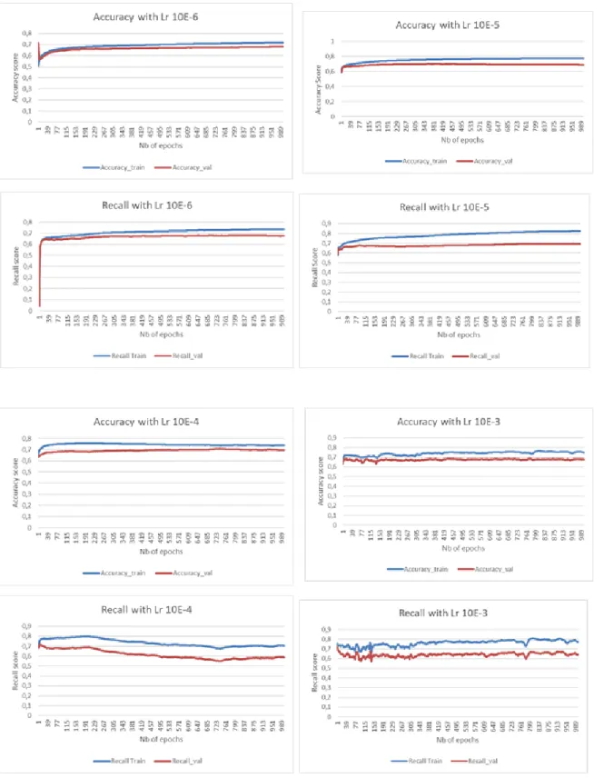
Figure 4.1 Accuracy and Recall Score depending the learning rate (continued) . 49 Figure 4.2 Accuracy and Recall Score depending the learning rate (continued and end) . . . 50

Figure 4.3 Normalized confusion matrix for Random Forest . . . 51

Figure 4.4 Normalized confusion matrix for Artificial neural network . . . 51

Figure 4.5 Normalized confusion matrix for Gradient boosted tree . . . 51

Figure 4.6 Normalized confusion matrix for Logistic regression . . . 51

Figure 4.7 Occurences for each classes . . . 61

LIST OF SYMBOLS AND ACRONYMS

EU European Union

GPS Global Positioning System

STM Société de transport de Montréal OTN Original Trip Number

HLP Haut-le-pied

AI Artficial Intelligence ML Machine Learning RF Random Forest

GBT Gradient Boosted Tree MLP Multilayer Perceptron SVM Support Vector Machine OD Origin-Destination

APTS Advanced Public Transportation Systems APC Automatic Passenger Count

AVL Automatic Vehicle Location ETA Estimated Time of Arrival RFID Radio Frequency Identification OTN Original Trip Number

UOTN Unique Original Trip Number TP True Positive

TN True Negative FP False Positive FN False Negative

ROC Receiver operating characteristic TS Time Slot

CHAPTER 1 INTRODUCTION

Public transit is a mass transportation system available to all and operated on defined lines and schedule, often managed by private companies under contracts of public instances. Public transport is from an economic and environmental point of view, the most effective means of transportation. Trains, subway, buses, and ferries are examples of public transport.

Several features are essential for a satisfactory public transport service, such as price, comfort and travel time. One of the most important features is the reliability of the scheduling, as stated by Peek and Van Hagen (2002) [1]. With the deployment of Advanced Public Transportation Systems (APTS), it is getting easier to gather information about the trip and thus to monitor the efficiency of the schedules.

Moreover, the cost of components giving access to real-time information about bus trips has decreased, which has led to a global deployment of these systems. The data extracted could help to improve the public transport service and reduce their costs.

1.1 Framework of the project

A definition of the basic concepts is essential to understand the project and to avoid misin-terpretations. To characterize the subject, the following sections will present the Montreal bus network and of the contractor in charge of managing the planning : GIRO.

1.1.1 Basic concepts and definitions

A bus is a transport facility which can transfer a limited number of people at the same time ; large buses can accommodate up to one hundred persons. A stop is a place where the bus halts along its way and where people can get in or out of the bus. A line is a collection of stops which determines a path from one terminus to another. A trip is a line covered by a bus, leaving a terminus at a determined time. A block is a sequence of trips that a bus covers between its start at a depot and its return. A layover is a buffer time during two trips of a block.

The figure 1.1 is an example of the schedule of a block. In this example, a bus is covering a sequence of 3 trips. The layover at the different terminuses serves the purpose of preventing the propagation of delays. When a bus finishes the last trip of a block, it comes back to the depot.

Figure 1.1 Concepts schematic

At the end of a trip, there are several possibilities : the bus can either do the same line in the return way, or stay at the same terminus and cover another trip, or go to another terminus and cover another trip. The trip intra terminus without covering any trip in the last option is called an Haut-le-pied (HLP) or deadhead.

1.1.2 Case study : the Montreal Bus network

The population of the island of Montreal is about 1,705,000 inhabitants in an area of 431,5 km2. The Montreal urban design is the superposition of an old urban division which comes from the French seigneurial period and the classic checkerboard pattern from North-American cities [2]. One of the characteristics of the road organization in Montreal is the few numbers of left-turn.

The Société de transport de Montréal (STM) administrates Montreal public transportation. In 2016, 221 bus lines were in activity, which represented about 4300 trips a day. Within the four subway lines, it is more than 429,5 million of travels during this year. The busiest bus lines could transport 31 777 people on average each day [3]. A new metro line is actually under construction and could be active for 2025.

The continental climate of the island of Montreal complicates public transport planning. Indeed, the cold winters damage the roads and make road works necessary during the rest of the year. It is an additional difficulty for the schedules of public transport.

More than a third of the vehicles in Montreal are equipped with APTS devices, mostly for passenger counting and GPS location over time. For each trip covered by a bus equipped with APTS devices, data are available at each stop, such as date, line number, direction, block

ID, trip ID, vehicle ID and the number of people in the vehicle. At each trip covering a line at a specific time is given an Original Trip Number (OTN). Furthermore, for each record, the scheduled time and the real departure time are available.

1.1.3 GIRO

The project has been done with the partnership of GIRO. GIRO is a Canadian company foun-ded in 1979 which provides software solutions for Public transport and postal organizations to plan, optimize, and manage their operations. Its clients are all over the world (the STM in Montréal, the SNCF in France, MTA in New-York, SBS in Singapore...). GIRO is providing the software Hastus to the STM in order to help in the scheduling and the operations. This software could manage a fleet of more than six thousand vehicles.

One of the current GIRO challenges is to integrate machine learning tools in their solutions for improving the reliability of their schedule, predicting the delay or the absence rate among the drivers. For that purpose, it has developed a partnership with universities and Research Chair, such as the Canada Excellence Research Chair in Data Science for Real-Time Decision-Making.

1.1.4 Machine Learning

Articial Intelligence (AI) is a field of computer science and was first introduced in 1956. AI includes all the theory and practices about creating things able to reproduce intelligence. Machine Learning (ML) is one of the study fields of AI. ML is based on a statistical approach in order to allow computers to improve their way of solving problems by themselves. The implementation of such methods is an essential part of ML.

In the first part of a ML implementation, the objective is to model an existing database. The model uses features as inputs and targets as outputs. This phase is called the learning phase. The second part is to try to predict future outputs using a combination of features. The learning can be supervised if the desired predictions are known : for example classification or regression. However, on the contrary, the learning is qualified of unsupervised if the objective of the learning is to determine and define the structure of the data [4].

There are several ML kinds of models : decision trees (which include Random Forest (RF) and Gradient Boosted Tree (GBT)), Support Vector Machine (SVM) or Artificial Neural-Network (ANN), just to quote some.

1.2 Problem

Deciding of the problem of the thesis was one of the main difficulties of the project. Indeed, at the beginning of the project, the framework was not specified. The first objective was to get ideas of various projects and determine their potential in term of machine-learning and their feasibility.

As the service quality is one of the main issues for public transportation planners and because GIRO is one of the main actors in this sector, it was decided that the project would aim to improve service quality.

An analysis of the available data led to the first outline of a problem : forecasting the delay at each stop using real-time data. However, the literature review showed that this problem was addressed by several before. Moreover, GIRO acts upstream in the public transportation system, and no real application could be found. Working with off-line data was essential for the project. Then, the idea of working with the layover appeared.

The analysis of the data shows that the scheduled time is not always respected, and the delay could be propagated inside a block. The layover, which is a buffer time, could prevent the propagation of delay. Thus it was thought that a new method to find adequate layover could be developed.

The layover is the main leverage a public transport planner could use in order to prevent delay propagation. Predicting the departure status of the trip was then the new objective of the thesis. However, once the situation is modeled, it just described the adequacy of the layover in this particular situation, and the importance of the feature layover was too significant. It was too difficult to transpose the models to other periods. The final idea was to forecast the delay of the end-trip, in order for public transport to have an idea of the necessary buffer time to prevent delay propagation.

1.3 Objectives

The first objective of this project was to determine the potential of the available data in machine learning processes. To decide it, an analysis of the different features was necessary. This analysis led to decide the other objectives of the projects.

The second objective was to find out if it was possible to model the end trip delays using offline data in Montreal. The data used come from Autumn 2017. Different machine learning models were candidates for this. Both binary and multi-label classifiers models were tested. Then the next step was to try if it was possible to train the different models on one period

(Autumn 2016) and test it on another (Autumn 2017). The objective of this part was to assess the possibility to predict end trip delays for future periods.

The ultimate objective of this thesis was to prepare a final deliverable for GIRO, predicting the probability distributions of delays for the different trips to help to create more reliable schedules. These distributions were compared to a normal distribution.

1.4 Work overview

This dissertation displays the work done to estimate the bus end trip delays. It also shows examples of how these models could be used practically. The thesis which presents this work is composed of different parts.

The first section presents a literature overview of the several topics of this thesis : the schedu-ling, arrival time prediction models, service reliability and APTS technologies. The analysis of arrival time prediction models shows that the use of only scheduling data had not been done yet, and this paper offers to fill this gap.

The second chapter describes the methodology and the several sources used to create the database. An analysis of the database is presented, as the correlation between the different features.

The third chapter describes the building and the optimization of the machine learning models which were used to estimate the delays for the various trips of the schedule. This chapter first presents binary classifying models and the second part describes multi-label ones. The last section shows the results of a model fits on one period and tested on another one. The algorithms are compared with a metric combining accuracy and recall : f1 score.

The fourth chapter presents the proposed method to assess schedule reliability. The trips are aggregated by time slot, line, and direction, and the probability distribution for the different delay classes are proposed. An analysis of the distance between the different probability distributions and reality described by frequencies in each category is presented.

Finally, the thesis concludes with the best of the algorithms presented in this work which could be used to predict bus end trip arrival times and proposes ideas for future work.

CHAPTER 2 LITERATURE REVIEW

2.1 Public transport planning

The public transport planning decomposes in several sub-problems [5]. The first one is esti-mating the demand, the second one is deciding the network design, the third one is creating the vehicle scheduling and the last one is the driver assignment. The following section will describe currently operated algorithms used to answer these different problems, such as the various factors essential for quality service in public transportation.

2.1.1 Planning methodology

The demand is often estimated by analyzing the previous data and estimating the habits of people. Origin-Destination (OD) matrices are used to model the demand, by estimating the number of people susceptible to go from the various origins to the different destinations. The OD matrices are created depending on the time of the days and are the best ways of estimating the needs of the public transportation network. Such matrices could either be created in static or dynamic way [6]. External factors such as fares or quality of the service should be taken into account to improve their accuracy [7].

Designing a network is a problem which aims at deciding the topology and the frequency of the operated lines to fulfill the demand under constraints of budget [8]. The routes and their recurrences can be assigned either separately using a first route set generation and genetic algorithm [9] or simultaneously [10]. The genetic algorithm also enables multi-objective and creates routes from scratches and produces results near to the Pareto optimum [11].

The vehicle scheduling problem aims at assigning buses to trips to cover a given timetable, taking into account the bus fleet and other practical constraints, such as the number of depots [12]. This problem is more complex than a routing problem because it has time windows as constraints [13]. The layover, or buffer time, is thus one of the leverages for having robust schedules. The algorithm produces sequences of trips which should be covered by buses, also called block. It is in this aspect of public transport planning that the project took place.

The last phase of the problem is driver assignment. Two elements composed this question : the first one is the creation of the different work days and the second one is to assign drivers to these work days, under some constraints such as collective agreements or workers availability. This problem is called the bus driver scheduling problem [14].

2.1.2 Quality factor for planning

Several factors can lead people to use public transportation [15]. These factors are :

— the fare of the public transport ticket, which supports the service provided. However the price is not the factor of the decision in itself, but the difference of expense in comparison to other transport solutions such as the bike or the car.

— the accessibility, in space which is the distance minimum to reach access to the public transport network, and in time which is the waiting time before accessing the facility — the mean travel time from one origin to a destination. It also has to be compared to

the travel time with other transport facilities

— the comfort of the passenger during the journey. The fact that some transports are overcrowded or outdated can have a fatal impact on the way people perceive public transportation.

— the safety

— the service reliability, which is how close the journey is to what expected the passenger. The thesis will develop this topic.

These various quality factors were prioritized in a Maslow pyramid by Peek and Van Hagen in 2002 as the figure 2.1 shows. Some quality factors could be qualified either of "satisfier", which means that their presence could encourage more people to use public transport, or "unsatisfier", which means their absence could prevent people from using public transport.

Figure 2.1 Quality factors in public transport presented in pyramid of Maslow (source : Peek and Van Hagen 2002)

Most people still uphold to use the private motor vehicle because of its convenience, despite the environmental degradation. Studies have shown that four major study fields will help to understand how to make people shift from private car to public transportation : improvement in service reliability, creating new evaluation methods, studying specificities of car users and how to make people perceived the benefits of public transportation [16].

2.2 Advanced Public Transportation Systems

APTS are a sub-class of Intelligent Transportation Systems which were defined by the Euro-pean Union (EU) Directive 2010/40/EU as systems where communication and information manage users, traffic flows, infrastructures and transports [17].

There are different types of APTS, also called intelligent public transportation Systems. The main advantage of using APTS technology is that the data could be collected automatically, and thus not having manual data collection efforts. APTS aims at enhancing efficiency and effectiveness of public transportation infrastructure, using archived data [18] [19]. The fol-lowing sections will present different APTS systems and how the analysis of the data they provided have improved service quality.

2.2.1 Automatic Passenger Count

For instance, many transit authorities throughout Canada and the United States used Au-tomatic Passenger Count (APC) technology [20]. APC systems can count the number of people using a set of infrared beams which cross stairwells at waist level. Passengers who are boarding or leaving break the beam and so close the switches : systems can count and record the passenger activity. Treadle mats can also be used to count the number of people entering and leaving public transports [21].

More recent counting passengers systems are developed, and they include tracking and vali-dation to people detection. These methods use various image recognition methods, detecting clothes and physical characteristics. They perform well on dense and sparse crowds and can identify more than 20% accurately than other competitive methods [22]. Stereovision can also be used to count the number of passengers in buses and subway [23].

There are multiples objectives in counting the number of people in public transports : moni-toring user trends, analyzing performance and identify problematic locations [21].

APC systems have been assessed, and measurement errors exist. However, the percentage of errors with APC systems is not relevant compared to mistakes made during manual data collection techniques [20].

2.2.2 Automatic Vehicle Location

Automatic Vehicle Location (AVL) use Global Positioning System (GPS) devices to track in real-time a whole fleet of buses. These AVL systems were designed at first for monitoring buses in real-time [24], but now it also provides data for offline analysis. AVL systems offer a

large amount of data which enable to track the percentage of schedule adherence at each stop and combine with APC data could even connect to the number of customers affected [25]. The schedule adherence is the percentage of buses which arrives within a time window near the schedule one and acceptable for the user. A poor quality schedule adherence can prevent passengers from using public transportation. AVL data can determine the statistical distri-bution of arrival time at each stop, and so update the transportation times in the timetables, and thus improving transit on-time performance [26]. Another example is the use of AVL data to detect bottleneck in public transportation networks [27].

Even if AVL systems are used to monitor the adherence to a schedule, they can have impacts directly on the willingness of the operator to keep on schedule, and thus on the schedule adherence directly [28].

2.2.3 Smart card

A smart card in public transportation is an electronic device which serves as a proof of sub-scription or automatizes fare collection systems. The predominant technology used actually in the smart card is Radio Frequency Identification (RFID). Transit agencies used them increa-singly because of their efficiency and effectiveness. While collecting payments, they produce large amounts of data which could compare planned and real trips arrival time or count the number of people onboard. The biggest challenge for this technology is to link the different trips made by a user to map their whole journey [29].

Smart card data coupled with cellphone call detail can provide patterns for urban mobility and transport mode choices, and thus find problematic locations which could prevent public transport usage. This method of data mining to determine temporal and spatial variability in transport mode preference has been tested on Singapore [30]. Moreover, mobile phone data give the ability to transit operator to improve the management of their service by monitoring the real demand with the one planned. Travel patterns can be found using mobile phone location data, and then provide accurate OD demand. New routes and schedules which could reduce both travel time and waiting time can be identified [31].

2.3 Service reliability

Improving service reliability could lead more people to use public transports. Moreover, public transport planners try to maximize it. This section describes the service reliability and focuses on schedule reliability.

2.3.1 Definition of service reliability

Service reliability can be defined as the difference between the expected service in time and comfort relative to the one perceived by the user. The time reliability can be assessed by the waiting time compared to the scheduled one. The comfort reliability can be evaluated by the possibility of finding a seat during peak hours and by the percentage of bus overcrowded. The degree of reliability relies mainly on the passenger assumption of the variability.

The planning robustness has been defined as the capacity of a schedule to respond to dis-ruptions without impacting the rest of the network [32]. The leading cause of disturbance in schedules is the presence of delays within the schedules, and thus planning robustness is directly linked to service reliability. Methods had been established to improve planning ro-bustness, which mainly consists of deciding the trade-off between the service quality, service reliability and operating costs [33].

2.3.2 Improving service reliability

One way of improving service reliability is by establishing holding points alongside the lines. Holding points are specific stops where the driver has to wait for a determined departure time to leave the particular stop if he is in advance. When holding points are employed, the additional travel time decreases [34].

Other factors can help in improving service reliability. For that, the STM has introduced smart card, has restricted some lane to bus-only use, has added articulated buses to its fleet and had integrated transit signal priority. Except for the transit signal priority, all the other solutions had positive impacts on service variation, a component of transit service reliability [35].

During the network design, transit planner can also improve service reliability by, for example, choosing line length and stop spacing. The waiting time can be decreased by 65% during the timetable design by optimizing the choice of the percentile value used. A too high value can improve the robustness of a model but can lead to extra waiting time for passenger between different stops [36].

2.3.3 Measuring service reliability

A measure of the service reliability can be done by counting the number of buses arriving within a time window near to the schedule one. However, for some tests, service reliability can be assessed as the number of buses arriving at the destination, regardless of the delay [37]. In the transit field, the ratio volume/capacity has been used to label critical points. A modern method to evaluate network performance has been developed, studying link capacity and network design [38]. This method had enabled more benefits than with the volume/capacity methods, by also quantifying the time saves.

Problematic links labeling is essential to evaluate the vulnerability of a public transport net-work. A robustness index has been proposed, using the capacity of the network for assessing the service performance [39]. This method locates critical links by using the change in all the network locations and can be used when the network robustness index is not significant.

2.3.4 Delay propagation and bus bunching

Several types of delay exist, such as the current delay, the primary delay (a bus ends a trip late) and the secondary delay (which occurs when a bus ends late a trip because the delay propagated). Cumulative distribution functions could model all of these delays. Thus, it has been possible to represent the delay propagation with an activity graph [40].

Using layover as buffer times could prevent a primary delay from propagating, and thus avoid further problems. Indeed, because of a primary delay, the number of people at each stop waiting for a bus will increase, and thus the probability of stopping at each stop and the dwell time will extend, generating more delays, causing the headway with the next bus to shrink. This phenomenon is called bus bunching. Some researches have tried to use APTS data to determine the causes of bus bunching [41].

Due to delay propagation, passengers could experience several negative aspects : changes in expected travel times, augmentation of the probability to find a vehicle crowed and the impossibility of finding a seat [15].

2.4 Predicting Delay in Public transportation

The main objective of the project was to estimate the end trip delay of trips. The following sections will review different methods used to predict travel time and forecast end trip delays, using various types of data.

The data collected through APTS have enabled the building of accurate models for bus travel times predictions and thus have improved the robustness of schedules. There are various factors which impact on bus travel times : some can be anticipated when designing networks such as the hour of the day and the route, but others cannot, such as weather conditions, traffic accidents or special events. Arrival time has been estimated using various methods, which mainly use real-time data.

2.4.1 Models using percentile methods

The most straightforward method to predict the travel time in public transportation is the use of the percentile travel time method. Using the 95th percentile travel time method indicates that 95 percent of the trips have a travel time shorter than the 95th percentile travel time. However this method is not accurate because generally the trips are not distinguished, and thus this method does not take into account exterior information such as the peak hours.

2.4.2 Models using historical data

Historical data models analyze travel time on the previous trip at the same period to forecast the bus travel time, assuming the traffic journey to remain stationary. Patterns could be found for traffic conditions on a daily and weekly basis, and the forecast could be done accurately for buses arrival time for part of the day, for each day of the week [42]. However, these models cannot take into account the subtleties of traffic.

Models could also use previous average travel time to predict further bus arrival time. This method was mainly used as a reference for other studies. This model was almost every time outperformed by the algorithm proposed by these researches [43]. Other inputs can be taken into account to adjust the results and improve accuracy. The main other independent feature which could be added to the model is the weather condition. Previous travel times can also be combined with dynamic data sources such as AVL systems to develop real-time prediction algorithm [44].

Another historical data model uses the average speed of vehicles over certain links of a route to forecast the Estimated Time of Arrival (ETA) of buses. Different algorithms have been

proposed to estimate bus arrival time extracting the average speed from GPS data [45]. A variation of this model has been proposed latter, combining real-time location, real-time traffic, historical travel time, temporal and spatial variations of the traffic conditions [46]. The main factor for the ETA of a bus is its current speed.

The previous models use historical data to make direct forecasts depending on the part of the day. The results could be made more accurate using a Double-Seasonal Holt-Winter’s Exponential Smoothing approach. This method allows the model to update itself with four different parameters and thus can take into account seasonality and time-trend in data series. The results show that estimation is approximately 10% better than elementary statistical models [47].

Models using historical data require a considerable set of data which cannot be available. Therefore, these models are not suitable for analysis with too significant variances in the differences in speed or travel times.

2.4.3 Models using statistics

The different factors which impact on bus arrival time are the diver behavior, signal, num-ber of people on the bus. These variables are used as independent ones in the majority of the studies, and the accuracy of the methods rely on their independence [48]. Most of the literature about statistical models have been published before the 1990s.

One of the statistical model used to forecast the ETA of buses is the use of time series. This model uses arrival time from historical periods to predict future arrival times. It is assumed that mathematical functions can provide patterns to determine arrival times, and these patterns will not change in the future. Precision for this model relies mostly on the likeness between previous and actual patterns [49]. Time series were not tested during the project because they need real-time data and we used offline data.

Another statistical model is using a regression model, and it is more likely to work under uncertain traffic condition. These models measure simultaneously the effects of various inputs in order to predict bus arrival times. These inputs can come from APC systems. Distance, boarding passengers, number of stops and weather information were used in various multi-linear regression to estimate bus arrival time at terminus [50]. One of the main advantages of regression is revealing the impact of each feature in the model. However, these models are usually outperformed by other models because the input data are highly inter-correlated [49]. This method is relatively easy to implement and was thus used as a comparison to the different machine learning models during the project.

2.4.4 Models using Machine Learning

There are several advantages of using ML models over statistical models. It is easier to deal with interdependent features in input and noisy data can be processed [51]. ML models are used without processing traffic data. However, results for one stop are not assignable to another location because of location specificities. The different machine learning algorithms implemented during the project are ANN, GBT and RF, and are presented in the following sections. SVM models are also described.

ANN have been recently more used for estimating bus travel time because of their ability to model any kind of function, even non-linear one. ANN models predicting end-trip arrival time has been proposed, using only GPS data, trained with historical data and test with real-time information. The ANN model outperformed the historical average model in term of prediction accuracy and robustness [52]. Jeong and Rilett also proposed an ANN model which performed better than multilinear regression models [53]. Furthermore, a model using ANN to predict bus travel time with GPS data and other features such as the number of passengers boarding had been proven efficient on a line of the Delhi public transport network [54]. The gradient boosting tree algorithm is a method based on decision trees, which creates new decision trees based on the errors made on the previous models. These new decision trees are therefore used to adjust the weight of data in the training set, to minimize a loss function. GBT algorithms have outperformed simpler model for travel time prediction [55]. However, the training time could be too considerable. GBT were also used in a method based on predicting the travel time of the different journey segments of a trip. This method also uses queueing theory estimators [56].

SVM is a recent neural network algorithm which tries to find the separating border between different output in order to classify them. The main advantage of SVM is the model find without specific function the relation between input and output. SVM models have been tested using three features : the segment, the travel time of the ongoing section and the latest travel time of the next section. The results showed that SVM model could be used to predict bus arrival time [57]. However, significant problems can cause computation time issues. Bus travel time has also been estimated using real-time road traffic with a SVM model, and this model has outperformed the ANN model [58].

RF algorithms create a specified number of decision trees during the training phase, and for multi-label classification, output the class represented the more in all the decision trees generated. RF models can also be operated for labeling bottleneck in public transport net-work by estimating a probability distribution for congestion in time and space [59]. This

algorithm manages to reduce the prediction error on congested days by 38% compared to a genetic algorithm. Another use of a RF algorithm for public transportation is to predict bus travel time using the near neighbor method [60]. This article demonstrates that even the computation time is slow, the model obtains a high accuracy. RF models have also been used to predict the service reliability of a bus line directly in Dalian (China) by estimating the punctuality, frequency and load factors of the buses [61].

Other machine learning algorithms exist and could have been tested during the project. For example recurrent neural networks, which are a class of artificial neural networks. However, this model is more specific for problems with temporal dynamic behavior and was not well suited for a model with offline data.

2.4.5 Models using Kalman Filter

Kalman filters were adopted along the years for many technologies using treatment signals, such as radar or communication. A Kalman filter uses the dynamic of an object to deduce its static characteristics, hence eliminating the noise of signals. These data can be used for studying the past, analyzing the present or predicting the future.

In some models Kalman filters had been incorporated to predict the expected bus arrival time at individual bus stops, using the filter to make the data more reliable and a neural network for the robustness [62]. Kalman filters can also integrate data from social networks in which people posted news about events they witnessed [63]. This method had been tested on a traffic simulator.

Kalman filters are used for preprocessing the data in models which also combine machine learning. Indeed, Kalman filters clean the data and make them more accurate, which help many machine learning models, especially with real-time data.

2.4.6 Conclusion

Different machine learning models can use APTS data in order to estimate bus arrival time, and they outperformed other models. Techniques such as Kalman filters can improve more the accuracy of the models. However, it has only been used for real-time prediction and not for the estimation of planning overall. The main advantage of machine learning models is that they find some patterns that human could not distinguish.

In this project, machine learning models will be trained on historical data on a planning level, in order to predict future periods, and will be compared to real-time data coming from APTS systems.

CHAPTER 3 DATA ANALYSIS

The database is an essential aspect when creating a machine learning model. Data could be collected from one or multiple sources, linked altogether, cleaned and then preprocessed before being operated in the models. This chapter presents the procedure which has led to the creation of the database. Therefore the database is analyzed, and the importance of the features is discussed. GIRO provided the data used in this project, which were extracted from the APTS systems installed by the STM in their fleet. They concern the period of the Autumn 2017 and Autumn 2016 for the buses in Montreal. As the data from Autumn 2016 were only used for a specific analysis, it was not investigated during the data analysis. However, the methodology to build it was the same as for Autumn 2017.

3.1 Planning Data

In public transportation, the planning is a document which displays the details about the trips scheduled, which means the departure time for the different lines. It also arranges the trips in sequence, called blocks. Moreover, it specifies the time of departure from the depot, the return to the depot and the HLP.

The schedule for Autumn 2017 was operated from the 28th of August until the 29th Octo-ber, for the weekdays and except the 4th of September and 9th October which were public holidays. In total, data from 43 days composes this database. Furthermore, 19 355 trips were scheduled for each weekday in Montreal during the described period. Hence the Autumn 2017 schedule can be used to describe 831 405 unique trips.

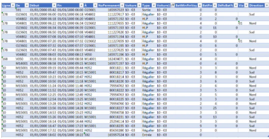
Figure 3.1 shows an example of data from the planning provided by GIRO.

The documents were available under several formats, and the format Comma-separated values (CSV) was used and transformed under XLSX files. The different elements available in the planning files are :

— the id of the line operated. The data can be missing if the bus is operating a return to the depot or an HLP for example. For the second record of the previous figure, the line ID is "178".

— the id of the origin of the trip. For the second record of the previous figure, the origin is "O23601".

— the scheduled start time of the trip. For the second record of the previous figure, the start time is "06 :00".

— the scheduled end time of the trip. For the second record of the previous figure, the scheduled end time ID is "06 :18".

— the id of the destination of the trip. For the second record of the previous figure, the Id of the destination is "V04802".

— the permanent number. This number is specific to each trip, and thus be considered as a primary key because it identifies uniquely every trip. For the second record of the previous figure, the permanent number is "111227617".

— the block id. For the second record of the previous figure, the block ID is "10 - 03". — the type of the trip. It can be either "regular" when it the bus operates a line, or "exit"

when the bus leaves the depot, or "return" when the bus comes back to the depot or "HLP" which are the bobtails. For the second record of the previous figure, the trip is "Regular".

— the minimum layover time in minutes. For the second record of the previous figure, the minimum layover time is "2".

— the actual layover. For the second record of the previous figure, the minimum layover time is "0".

— the shortfall layover, which is different from 0 if the actual layover is lower than the minimum layover. However, this situation does not exist in our database. For the second record of the previous figure, the shortfall layover time is not indicated. — the deviation, because buses can follow different paths for the same line, for example

for a special time of the day. For the second record of the previous figure, the deviation is not indicated, which means that the bus follows the classic path.

— the direction, which can be one of the four cardinal directions. For the second record of the previous figure, the deviation "South".

The layover is not always indicated because if an HLP follows a regular trip, the layover will be transferred at the end of the HLP. The minimum layover time comes from the 95% percentile method, which means that if the minimum layover is satisfied, at least 95% of the trips would start on-time. However, this method is not very robust.

One trip is unique for each day, and its primary key is the permanent number. During the project, it was slightly modified and called OTN. A primary key composed of the day number aggregated to the permanent number was created to identify each trip in our database uniquely. The id created was named Unique Original Trip Number (UOTN).

3.2 APTS Data

The APTS data provided by the STM data center are a mix of AVL and APC data. They were recorded via a system called SCAD. In the data furnished, manually collected data were present but were removed.

3.2.1 Raw data

The gathered data were transferred upon a CSV format. One record gave the information of a bus making a halt at a bus stop, and various precise details such as the actual time of arrival and the number of people boarding and leaving the bus. Figure 3.2 is an example of a file provided :

Figure 3.2 Example of APTS file

The different details present for one record are :

— System Record Number, which is the id of the record. The first record of the example has a system record number of "139814965".

— Date. The first record of the example has a record data of "28/08/2017".

— Original Trip Number. The first record of the example has an original trip number of "135388586".

— Route id. The first record of the example has a route id of "139".

— Direction, which is an integer between 0 and 3. North is associated with 0, South to 1, East to 2 and West to 3. If a record has no direction associated, it is because the record is related to an HLP. The first record of the example has a direction of "0", which means "North".

— Block Id. The first record of the example has a block id of "139-44".

— Stop Rank. The first record of the example has a stop rank of "9", which means that the record corresponds to the 9th stops of a line.

— Stop id. The first record of the example has a stop id of "120036".

— Scheduled time. The first record of the example has a scheduled time of "1109400" in the STM time convention.

— Arrival Time. The first record of the example has an arrival time of "1109740" in the STM time convention.

— Departure Time. The first record of the example has a departure time of "1111070" in the STM time convention.

— Number of people boarding. The first record of the example has 97 people boarding. — Number of people debarking. The first record of the example has 15 people debarking. — Number of the passengers on the bus. The first record of the example has 106

passen-gers on the bus.

— The source of the record. The first record of the example has "SCAD" as a source, which means it was recorded via the APTS system.

— The location of the record. The first record of the example has a location of "120036", which is the same as the stop id.

The format of some columns was modified in order to simplify further analysis. Moreover, some features were added to the database : the day of the week (from Monday to Friday), the part of the day or the UOTN associated to the record to link it later to planning data. The part of the day was decided as follow : "P" to describe peak hours, from 6 am to 9 am and from 3 pm to 6.30 pm, "T" for transition hours which are the 30 minutes before and after each peak hours, and finally "N" for the other period.

Also, the time was transformed in order to appear in a second format. The STM time conven-tion gives the time tenth of second, with a day starting at 432 000. The first record which has a scheduled time of 1109400 could be converted in second :

T (s) = 1109400 − 432000

10 = 67740

Thus, 1109400 in STM time convention is 67 740 seconds, or 18 :49 :00, or 6.49 p.m. The figure 3.3 is an example of the APTS file cleaned.

Figure 3.3 Example of APTS file cleaned

3.2.2 Extracting trip info

The topic of the research is to estimate end-trip delay for buses. Hence only one record for each trip was relevant : the last one. The last record of each trip was extracted via a Macro VBA. As the interest of the research is to work with planning, real-time data such as the number of people in the buses were not collected. The figure 3.4 shows a file treated with a Macro VBA. Lots of information were redundant with data present in the planning file, thus only the scheduled time and the arrival time were extracted, as well as the UOTN and the OTN in order to link the data. The times are in second.

Figure 3.4 Example of information extracted from APTS data

All the 43 files were treated with this method. Finally, 139 452 trips were collected. Moreover, as explained before, 19935 were scheduled each day, which implies that 831 405 trips could have been recorded. The difference is explained by the fact that only 20% of the buses were equipped with SCAD systems in 2017 [3]. 20% of the 831 405 scheduled trips is 166 281. Thus the number of trips collected is coherent.

3.3 External information

Once the planning and APTS data were gathered, other sources of information were analyzed to add features to our model. New data had to be off-line information, as the objective of the project is to work with planning data and not in real-time. GIRO provided additional information involving stops information, driver schedules and layover time.

3.3.1 Stop info

The objective of having stop information was dual : on one hand to have geographic infor-mation for the terminus, and on the other hand to know the road taken by the different lines.

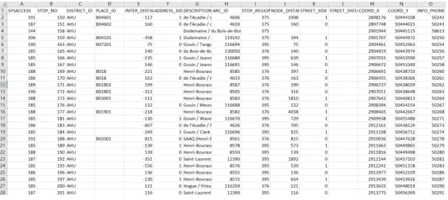
The file received was a CSV file composed of the stops id and their characteristics, as shown in the figure 3.5. The information used was in the columns districts and coordinate X and coordinate Y. A change in the format had to be done to normalize it. In order to link this data with the planning data, the place Id was used. The range of the value goes from 2,69 to 3.06 for X coordinates, and from 5,029 to 5,062 for the Y coordinates.

Figure 3.5 Example of Stop file

3.3.2 Driver change

Driver schedules could be decided during the planning phase, and so could be integrated into the features. One driver can do several blocks in a working day, and several drivers could operate one block. In the figure 3.6, the id in the column "journée" means that a unique operator was operating all the trips having this id in characteristic. Having a change of driver during a block could imply delays if the new driver is late for different reasons.

3.3.3 Mean Layover Prev

The layover time is a buffer time which can prevent the delay propagation. Hence it is interesting to have information about all the previous layovers. Thus the mean layover of the previous trip was calculated. A sum of all the layovers could have been done, but the information would have been correlated to the block rank. When the trip was the first of the block, instead of letting a blank, a decision was made to choose 20 minutes, which is a high value, similar to a one which would prevent delay propagation. This choice emphasizes the fact that there is no delay propagation for the first trip of a block.

3.3.4 Day of the week

The information about the day of the week was also extracted. Only the weekdays are present.

3.3.5 Creating the final database

Finally, all the information were gathered in a final database, and the followinf figure gives an overview.

Figure 3.7 Example of Final Database file

3.4 Preprocessing

Once the database is created, a preprocessing work was done to prevent unreliable information to be part of the database. Indeed, it is essential to have all the information for each record to afford machine learning models to find more accurate patterns between the data.

3.4.1 Missing data

When the stop information was linked to the database, the coordinates of ten different stops present in the database were missing. These stops were extracted and analyzed by the routes they come from. It appears that because of the deviation of some routes, the end stop has a slightly different id and thus cannot be linked to the stop database. The id replacement was made, and the missing data were incorporated.

Also, 26 records from APTS data had UOTN which could not be linked with data from the planning. It represented four different OTN. Therefore these data were removed from the database. It was supposed that these trips were not planned initially and were added for special events or in support of public transport malfunction.

At this step, the database was composed of 139 426 records.

3.4.2 Database cleaning

To be sure the data from the APTS sources match precisely the planning data, the scheduled time for the last stop was also extracted with the macro VBA. It was found that 5176 extracted data had a scheduled arrival time which did not match with the one presents in the planning database. The explanation was possible malfunctions of the APTS devices, which could have stopped working at some points and thus not recording the last stops of a trip. As it represented less than 5% of the data, it was decided to remove these records from the database.

At this step, the database was composed of 134 250 records.

3.4.3 Remove the lines of less than 100 occurrences

In order to avoid to have a too unbalanced database, a decision was made to remove the records concerning lines with too few occurrences. Indeed, even if some methods had been developed in order to struggle with this issue, it is always better to have a balanced database. Figure 3.8 shows the number of occurrences for each line.

Figure 3.8 Number of records for each line

It was decided arbitrarily that trip describing lines with less than 100 occurrences would be removed from the database. Then, 3 769 records coming from 119 lines were removed. The remaining data reflected 184 lines. As it will be explained later in this thesis, the line feature is preprocessed with the one-hot method before being incorporated in machine learning models, and so decreasing the number of lines will improve the accuracy of the models and decrease the training time.

At this step, the database was composed of 130 481 records.

3.4.4 Conclusion of preprocessing

After these three steps, on the database of 139 452 records, 130 481 were used, which means that 9.4% of the data were removed. The table 3.1 synthesis the different steps.

Table 3.1 Synthesis of preprocessing

Step Comments Number of records in the database 0 Database initial 139 452

1 Missing Data 139 426 2 Unmatched Data 134 250 3 Lines with few occurrences 130 481

3.5 Database Analysis

Once the different features incorporated in the database, an analysis of the database was made.

3.5.1 Features Analysis

The different features of the database are synthesized in the table 3.2.

Table 3.2 Synthesis of the features Planning Data Other Data

Line (integer) Last Stop X (continuous) Block Rank (integer) Last Stop Y (continuous) Mean Layover Prev (continuous) Driver Change (binary)

Scheduled Time (integer) Week Day (integer) Via (binary)

Direction (integer)

The next sections will describe more precisely each feature.

Line feature

Figure 3.9 shows the partition after the preprocessing explained in the previous section.

The partition function is similar to a Pareto one.

Block Rank Feature

Figure 3.10 Number of records by block rank

The number of observation decreases when the block rank gets higher because if a trip is recorded, all the previous trips of the same block are also recorded.

Mean of the Previous Layovers feature

For each trip, the mean of the previous layovers of its block was calculated, except for the first trip of the block whose value was set to 20. The feature is continuous, and so to describe it, the different values were integrated into a class, calculated by making a superior rounding. For example, if a value was calculated at 3.2, the value was incorporated in class 4.

Figure 3.11 Number of records by Mean Layover Prev

The majority of the records have a mean layover prev included between 5 and 10 minutes. A large number of records with a 20 mean previous layover is explained by the fact that the mean layover previous feature had been set at 20 for the first trip of the blocks.

Scheduled time feature

As the feature is continuous, the values were gathered by time slots, which symbolize periods of 30 minutes. However, the values were integrated with a normalizing preprocessor in the machine learning models.

Figure 3.12 Number of records by time slot

They are two peak-time periods by day : one from 6 am to 9 am and the other from 3 pm to 6.30pm. They correspond to the time slot from 12 to 18 and from 30 to 37. These time slots are effectively the most represented.

Via feature

The feature is one if the line does not take the usual road, and 0 if it takes the usual one.

Table 3.3 Number of records Via Via Number of records

0 117 230

1 13 251

Around 10% of the trips recorded have taken a via road.

Direction feature