Modélisation du bilan hydrique à pas de temps mensuel pour l'évaluation de l'impact du changement climatique dans le bassin Amazonien du Pérou

(1)

T

H

È

S

E

En vue de l'obtention du

D

O

C

T

O

R

A

T

D

E

L

’

U

N

I

V

E

R

S

I

T

É

D

E

T

O

U

L

O

U

S

E

Délivré par l'Université Toulouse III - Paul Sabatier (UT3 Paul Sabatier) Discipline ou spécialité : Hydrologie

JURY

M. Jérôme Viers (Professeur UPS, Toulouse) Président Walter Collischonn (IPH, Porto Alegre) Rapporteur

Gil Mahé (IRD-MSE, Montpellier) Rapporteur Mme. Elizabeth Silvestre (SENAMHI, Lima) Examinateur M. Abel Mejia (Président UNALM, Lima) Examinateur

Mme. Sandra Ardoin (IRD-MSE, Montpellier) Invitée

Ecole doctorale : Sciences de l'Univers, de l'Environnement et de l'Espace (SDU2E) Unité de recherche : LMTG - UMR 5563 UR 154 CNRS Université Paul Sabatier IRD

Directeur(s) de Thèse : Jean-Loup Guyot,David Labat Rapporteurs : Gil Mahé et Walter Collischonn

Présentée et soutenue par Waldo Sven LAVADO CASIMIRO Le mardi 16 février 2010

Titre :

Modélisation du bilan hydrique à pas de temps mensuel pour l’évaluation de l'impact du changement climatique dans le bassin Amazonien du Pérou.

(2)

(3)

Résumé

Les recherches entreprises au cours de la présente thèse s’intéressent à répondre aux questions suivantes:

• Quels sont les cycles annuels et saisonniers, ainsi que la variabilité interannuelle et intra-saisonnière à moyen et long terme, des principales composantes du cycle hydrologique sur les bassins des rios Huallaga et Ucayali ?

• Quelles sont les réserves disponibles en eau sur les bassins des rios Huallaga et Ucayali ? • Quel est l’impact du changement climatique sur l’hydrologie des rios Huallaga et Ucayali ? En premier lieu, nous décrivons les principales caractéristiques des bassins des rios Ucayali et Huallaga, ainsi que la base de données utilisée. Nous avons ainsi mis en évidence le réchauffement sur notre zone d’étude (estimé à +0.09°C par décade). De plus, les ruptures observées sur les séries de température moyenne à la fin des années 70 concordent avec les séquences d’événements de type « El Niño ». Nous avons aussi démontré une corrélation négative entre les températures et l'indice du Pacifique (Indice d’Oscillation du Sud, IOS). Par contre, aucune tendance n’est mise en évidence dans les séries de précipitation. Néanmoins, environ 10% des stations de notre région d’étude présentent des ruptures significatives dans la période 1991-2000.

La production des ressources en eau sur les bassins des rios Ucayali et Huallaga est évaluée pour 7 sous-bassins : 6 situés dans le bassin de l’Ucayali et un situé dans le basin du Huallaga. Pour quantifier ces ressources en eau, nous utilisons deux modèles hydrologiques au pas de temps mensuel (GR2M et MWB3). L’utilisation des données de capacité de rétention en eau des sols (maximum, moyenne et minimum) de la FAO, comme valeurs d’entrée dans les modèles hydrologiques, a contribué à rendre plus physique ces modèles. Les paramètres optimaux obtenus par calibration reproduisent raisonnablement bien l'écoulement observé à l’exutoire des bassins sélectionnés.

L’impact des changements climatiques sur l’hydrologie ont été évalué en utilisant comme données climatiques les sorties des modèles de l’IPCC (BCM2, CSMK3 et MIHR), correspondant aux scénarios A1B et B1. Les écoulements annuels simulés sur la période 2008-2099 suggèrent que les impacts du changement climatique sur l'hydrologie varient avec le bassin, le modèle hydrologique choisi, et le scénario: Le sous-basin Requena est caractérisé par une augmentation (respectivement une diminution) d'écoulement en utilisant les modèles GR2M (respectivement MWB3) en considérant les scénarios A1B et B. Les bassins de Chazuta, Maldonadillo et Pisac voient leurs débits diminuer tandis que les bassins de Puerto Inca, Tambo et Mejorada voient leurs débits augmenter.

Les changements simulés dans les écoulements mensuels sur la période 2008-2099 suggèrent une augmentation pour tous les sous-bassins, excepté le bassin de Pisac. Juillet, Août et Septembre sont en général les mois caractérisés par les changements les plus marqués, avec une augmentation des débits pour les bassins de Requena, Chazuta, Puerto Inca, Maldonadillo et Tambo.

Mots Clés : bassin Amazonien ; Pérou ; variabilité hydroclimatique ; modélisation

(4)

Abstract

The researches developed during this study gives answers about three important questions: • What are the annual and seasonal cycles, as well as interannual and intra-seasonal variability in the medium and long term hydrological cycle over the basins of Huallaga and Ucayali rivers?

• What are the water resources available in the basins of Huallaga and Ucayali rivers?

• What is the impact of the climate change on the hydrological cycle of Huallaga and Ucayali rivers?

First, we describe the main features of the basins of Huallaga and Ucayali rivers, as well as the hydrological database used an we put in evidence a warming in our zone of study (estimated at +0.09°C per decade). Moreover, the ruptures observed in the series of average temperature at the end of the Seventies are in accordance with the sequences of “El Niño”. We showed a negative correlation between the temperatures and the index of the Pacific (Southern Oscillation Index, SOI). On the other hand, no tendency is highlighted in the precipitation series. Nevertheless, approximately 10% of the stations in our area of study present significant ruptures during the 1991-2000 decade.

Then, the production of water resources in the basins of Huallaga and Ucayali rivers is evaluated over 7 sub-basins: 6 located in the Ucayali basin and one located in the Huallaga basin. To quantify water resources, we use two hydrological models at monthly step (GR2M and MWB3). The use of water holding capacity data of FAO soils (maximum, mean and minimum) as input of the hydrological models, contributed to propose physical interpretations to these models. The optimal parameters obtained by calibration procedure reproduce reasonably well the flow observed in the selected basins. The impacts of climate change on hydrology were evaluated using as climatic data the outputs of the IPCC models (BCM2, CSMK3 and MIHR), corresponding to the scenarios A1B and B1. The annual flows simulated in the 2008-2099 period suggest that the impacts of climate change on hydrology vary with the basin, the hydrological model chosen, and the scenario: The Requena sub-basin is characterized by an increase (respectively a reduction) of flow using GR2M model (respectively MWB3) considering the A1B and B1 scenarios. The Chazuta, Maldonadillo and Pisac basins exhibit flows decreasing while the basins of Puerto Inca, Tambo and Mejorada show flows increasing. The changes simulated in monthly flows over the 2008-2099 period suggest an increase for all the sub-basins, except the Pisac basin. July, August and September are in general the months characterized by the most marked changes, with an increase in flows for Requena, Chazuta, Puerto Inca, Maldonadillo and Tambo basins.

Key words: Amazonas basin; Peru; hydroclimatic variability; hydrological models; climate

(5)

Resumen

Las investigaciones realizadas en la presente tesis se interesan en responder a las siguientes preguntas:

• ¿Cuáles son los ciclos anuales y estacionales, así como la variabilidad interanual e interestacional a mediano y largo plazo de los principales componentes del ciclo hidrológico sobre las cuencas de los ríos Huallaga y Ucayali?

• ¿Cuáles son las reservas disponibles de agua sobre las cuencas de los ríos Huallaga y Ucayali?

• ¿Cuál es el impacto del cambio climático en la hidrología de los ríos Huallaga y Ucayali? En primer lugar, describimos las principales características de las cuencas de los ríos Huallaga y Ucayali, así como la base de datos utilizada. Así, observamos un calentamiento sobre nuestra zona de estudio (estimado en +0.09°C por década). Además, las rupturas observadas sobre las series de temperatura media al final de los años 70 están en concordancia con el aumento de las frecuencias de los eventos “EL Niño”. También demostramos una correlación negativa entre las temperaturas y el índice del Pacífico (Índice de Oscilación del Sur, IOS). Para las series de precipitación, ninguna tendencia clara se pone en evidencia. Sin embargo, alrededor del 10% de las estaciones de nuestra región de estudio presentan rupturas significativas en el período 1991-2000. La producción de los recursos hídricos sobre las cuencas de los ríos Ucayali y Huallaga se evaluaron para 7 sub cuencas: 6 situados en la cuenca del río Ucayali y uno situado en la cuenca del río Huallaga. Para cuantificar estos recursos hídricos, utilizamos dos modelos hidrológicos al paso de tiempo mensual (GR2M y MWB3). La utilización de los datos de capacidad de retención en agua de los suelos (máximo, media y mínimo) de la FAO, como valores de entrada en los modelos hidrológicos, contribuyó a hacer más físico estos modelos. Los parámetros óptimos obtenidos por el procedimiento de calibración reproducen razonablemente bien los caudales observados en las cuencas seleccionadas. El impacto de los cambios climáticos en la hidrología se evaluó utilizando como datos climáticos las salidas de los modelos del IPCC (BCM2, CSMK3 y MIHR), considerando los escenarios A1B y B1. Los caudales anuales simulados en el período 2008-2099 sugieren que los impactos del cambio climático en la hidrología varían con la cuenca, el modelo hidrológico elegido, y el escenario: La cuenca de Requena es caracterizada por un aumento (respectivamente una disminución) de los caudales al utilizar los modelos GR2M (respectivamente MWB3) al considerar los escenarios A1B y B. Las cuencas de Chazuta, Maldonadillo y Pisac ven sus caudales disminuir mientras que las cuencas de Puerto Inca, Tambo y Mejorada ven sus caudales aumentar. Los cambios simulados en los caudales mensuales en el período 2008-2099 sugieren un aumento para todas las cuencas, excepto la cuenca de Pisac. Julio, Agosto y Septiembre son en general los meses caracterizados por los cambios más fuertes, con un aumento de los caudales para las cuencas de Requena, Chazuta, Puerto Inca, Maldonadillo y Tambo.

Palabras Clave: cuenca Amazónica; Perú; variabilidad hidroclimática; modelización

(6)

Remerciements

Je tiens en premier lieu à remercier très sincèrement et très chaleureusement mes deux directeurs Jean Loup Guyot et David Labat qui ont assuré la finalisation de cette thèse. Aussi je dois remercier très sincèrement à Josyane Ronchail pour m’avoir aidé pendant la fin de ma thèse. Finalement je remercie aussi Sandra Ardoin-Bardin par m’avoir aidé au début de ma thèse pendant mon premier séjour hors de Toulouse à la Maison de Sciences de l’eau de Montpellier.

Cette thèse financée par le Conseil National de Science et Technologie Péruvien (CONCYTEC), l’Ambassade de Françe au Pérou et l’Institut de Recherche pour le Développement (IRD) a été menée au sein du Laboratoire de Mécanismes et Transferts en Géologie (LMTG) à Toulouse et au sein du Service National de Météorologie et Hydrologie Péruvien (SENAMHI) à Lima. Je remercie leurs directeurs respectifs François Martin (LMTG) et Wilar Gamarra (SENAMHI) de m’avoir accueilli pendant le parcours de ma thèse. Au Pérou, je remercie le SENAMHI de m’avoir permis de passer mes séjours en France et à mes collègues de la Direction Générale d’Hydrologie et Ressources en eau pour m’avoir soutenu pendant le parcours de ma thèse. Je remercie aussi mes amis péruviens et « Molineros » Wilson Suarez, Jhan Carlo Espinoza et Fernando Vegas pour leurs conseils et temps passé avec eux en discussions scientifiques, politiques et de soirées bières au Pérou et en France. Je remercie aussi les membres du projet HYBAM au Pérou : Pascal Fraizy, Phillipe Vauchel, Jean Sébastien avec lesquels nous avons effectué des missions en Amazonie Péruvienne.

Toute cette histoire a commencé au début de l’année 2003 lors que j’ai fais ma première mission de jaugeages sur les fleuves amazoniens péruviens en tant qu’ingénieur du SENAMHI avec Jean Loup Guyot et Pascal Fraizy, mes collègues de l’IRD. Ensuite, j’ai eu la proposition de Jean Loup pour faire des études en France. Après deux ans de bataille, nous avons obtenu une bourse pour passer la première année de thèse en France. Après une année difficile en France j’ai eu l’occasion de connaître de très bons amis qui on rendu plus agréable mon séjour en France (Carolina, Teresa, Marcelo, Juan Gabriel, Matias, Joecyla, Michelly, Natalia, Pierre et d’autres pour lesquels je m’excuse par avance auprès d’eux si je ne les ai pas mentionnés). Après une année au Pérou, je suis revenu en France pour passer ma deuxième année de thèse, c’est ici que j’ai rencontré le bataillon des amis dont la plus part sont Chiliens avec qui j’ai passé de superbes moments de sport, de soirées, de pause-café et de batailles pour savoir l’origine du Pisco. Alejandro, German, Damian, Salvador, Carola, Jocelyn, Ana, Augusto et la plupart des autres mentionnés ci-dessus. Je remercie aussi Benjamin pour les matchs de tennis dignes de Roland Garros sur le terrain de l’OMP. Je remercie également mes collègues de bureau Laure, Marie et François Xavier pour m’avoir soutenu et pour leur compagnie très agréable.

Je remercie aussi l’ensemble des personnes au LMTG et au SENAMHI dont le travail ou simplement les conseils m’ont permis de mener à bien cette thèse et dont la liste est longue : il est difficile de toutes les citer ici au risque d’en oublier certaines. Je suis persuadé qu’elles se reconnaitront parmi celles à qui j’exprime ma profonde gratitude et mes sincères remerciements.

(7)

(8)

(9)

1

Table des matières

I. CHAPITRE 1. Introduction ... 8

1.1 Contexte général du Pérou ... 8

1.2 A basin-scale trends in rainfall and runoff in Peru (1969-2004): Pacific, Titicaca and Amazonas drainage. ... 11

1.3 Les programmes de recherche dans lesquels s’inscrit la thèse ... 29

1.3.1 Le programme HYBAM (Hydrogéodynamique du Bassin Amazonien) ... 29

1.3.2 Le SENAMHI (Service National de Météorologie et Hydrologie de Pérou) . 30 1.4 Sélection de bassins versants ... 30

1.5 Objectifs de la thèse ... 30

1.6 Organisation de la thèse ... 31

II. CHAPITRE 2 .Les basins de l’Ucayali et du Huallaga ... 33

2.1 Aspects climatiques ... 33 2.1.1 Précipitations ... 33 2.1.2 Température et Evapotranspiration ... 34 2.2 Aspects géomorphologiques ... 37 2.2.1 Relief ... 37 2.2.2 Géologie ... 37 2.2.3 Sols ... 39 2.2.4 Végétation ... 40 2.2.5 Aspects socio-économiques ... 41

2.3 Réseau hydrologique du SENAMHI et lesmesures hydrologiques récentes acquises dans le cadre du programme HYBAM ... 42

2.4 Sous basins sélectionnés sur les bassins Ucayali et Huallaga. ... 43

(10)

2

2.5.1 Données hydrologiques ... 47

2.5.2 Données pluviométriques ... 48

2.5.3 Données d’évapotranspiration ... 48

2.5.4 Données des sols FAO ... 69

2.5.5 Constitution des grilles ... 71

2.6 Conclusions ... 71

III. CHAPITRE 3 .Variabilité hydroclimatique sur les bassins des rios Ucayali et Huallaga ... 74

3.1 Recent trends in rainfall, temperature and evapotranspiration in the Peruvian Amazonas-Andes basin: Huallaga and Ucayali basins. ... 74

3.2 Variabilité spatiale des débits sur les bassins de l’Ucayali et de Huallaga ... 94

IV. CHAPITRE 4 .Modélisation de bilan hydrique au pas de temps mensuel et impact du changement climatique sur les régimes hydrologiques dans les basins des rios Ucayali et Huallaga ... 98

4.1 Premiers essais de modélisation en utilisant des modèles de bilan hydrique mensuel ... 98

4.1.2 Monthly water balance models in the Amazon drainage basin of Peru: Ucayali River basin ... 98

4.2 Modélisation au niveau mensuel sur sept sous-bassins des rios Ucayali et Huallaga, et évaluation des impacts du changement climatique sur le régime hydrologique .. ... 111

V. CHAPITRE 5. Conclusion générale et perspectives ... 143

5.1 Conclusion ... 143

5.2 Perspectives ... 145

5.2.1 Validation des autres sources de données de pluie sur le basin amazonien péruvien. ... 145

5.2.2 La modélisation hydrologique au pas de temps journalier ... 145

(11)

3

5.2.4 L’impact du changement hydrologique au niveau journalier sur l’hydrologie. . ... 145 5.2.5 Autres perspectives ... 146 Bibliographie ... 147

(12)

4

Liste de Figures

Figure I-1. Gauche : relief du Pérou en altitudes (http://geografia.laguia2000.com). Droite :

république du Pérou en Amérique du Sud au 1er janvier 2009 (http://fr.wikipedia.org/wiki/fichier:south_america_location_per.png). ... 9

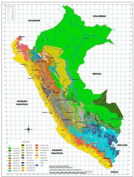
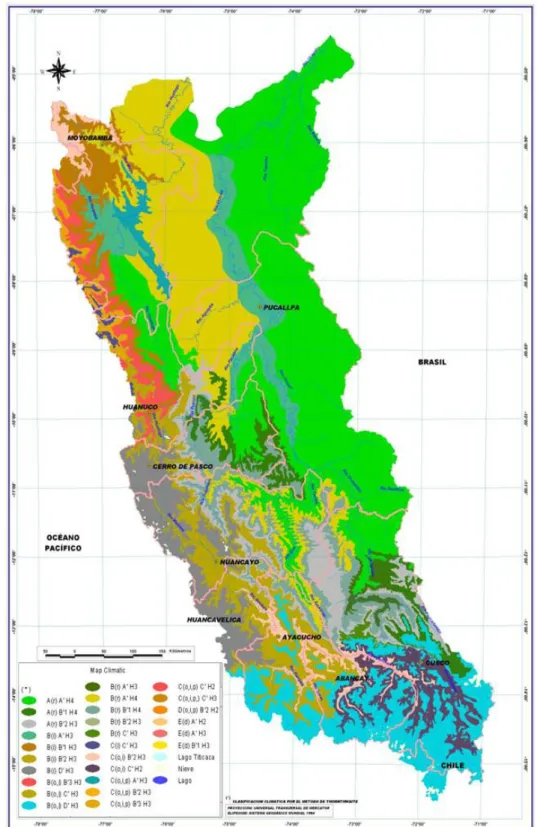
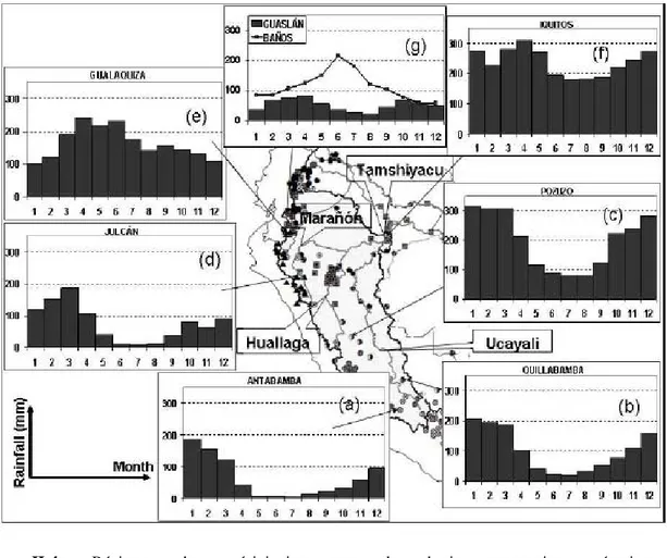
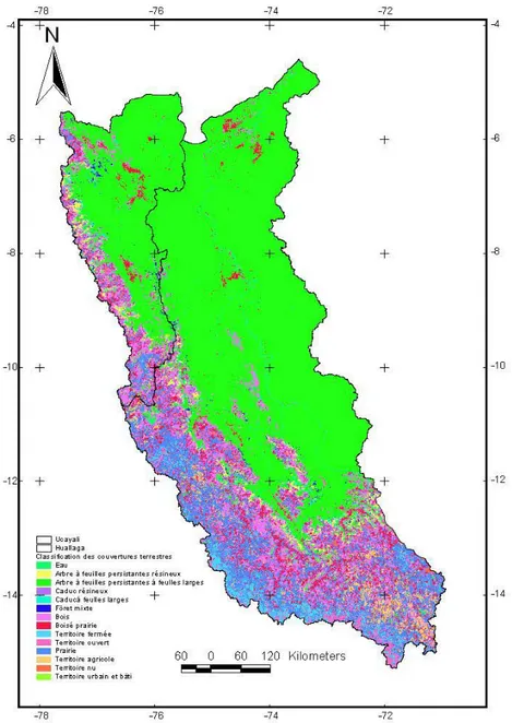
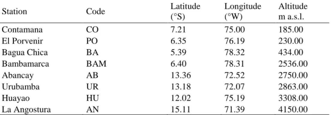
Figure I-2. Classification climatique du Pérou en utilisant la classification de Thornthwaite (d’après SENAMHI, 2005. Voir Tableau I-1). ... 10 Figure I-3. Versants du Pérou : Versant du Pacifique (ouest), Versant du Lac Titicaca (sud est) et Versant de l’Amazonas (est). (D'après UNESCO, 2006). ... 12 Figure II-1. a) Localisations des bassins de l’Ucayali et du Huallaga au Pérou. b) Fleuves sur le drainage du bassin Amazonien avec les fleuves Ucayali signalé (ligne violette) (d’après :http://fr.wikipedia.org/wiki/Fichier:Ucayalirivermap.png). c) Comme b mais pour le fleuve Huallaga (d’après http://fr.wikipedia.org/wiki/Fichier:Huallagarivermap.png). ... 34 Figure II-2. Classification climatique des bassins Ucayali et Huallaga en utilisant la classification de Thornthwaite (d’après SENAMHI, 2005, voir Tableau I-1). ... 35 Figure II-3. Carte des climats moyens interannuels. a) Pluie ; b) Température moyenne ; c)Température maxime ; d) Température minime et e) Evapotranspiration. Ligne pointille divise les Andes (est) et la Forêt (ouest). ... 36 Figure II-4. Régimes de précipitation sur la basin amazonien péruvien (d’après Espinoza et al., 2008, voir Annexes). ... 36 Figure II-5. Carte des altitudes sur les bassins des rios Ucayali et Huallaga. ... 38 Figure II-6. Types de sols identifiés sur les bassins des rios Ucayali et Huallaga. Pour la légende voir Tableau II-1. D’après FAO/UNESCO (1981). ... 41 Figure II-7. Carte de végétation des bassins des rios Ucayali et Huallaga. ... 42 Figure II-8. Division politique des bassins des rios Ucayali et Huallaga. Les bassins de l’Ucayali et Huallaga sont limités par la ligne noire. ... 43 Figure II-9. Réseaux des stations hydrométriques du SENAMHI avec mesures des débits jusqu’en 2001. Les stations sont identifiées par des carrés rouges et violets. D’après UNESCO, 2006. ... 44 Figure II-10. Réseau des stations hydrométriques du SENAMHI avec mesures de débits, par le programme HYBAM (IRD-SENAMHI-UNALM). ... 45 Figure II-11. Bassins sélectionnées pour notre étude. Pour la description voir la Tableau II-2. Les croix grises permettent de localiser les stations de mesure des précipitations tandis que étoiles noires indiquent les stations de mesure des températures. ... 46

(13)

5

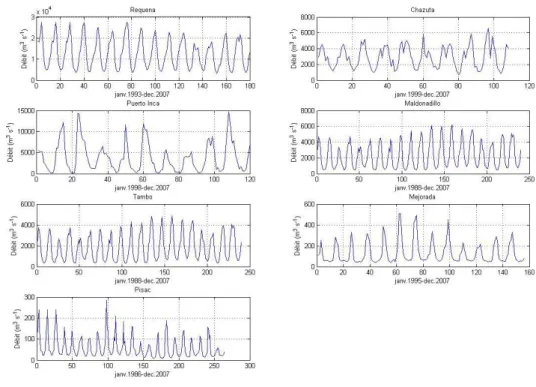
Figure II-12. Séries mensuelles des débits des stations hydrologiques retenues pour la présente étude. ... 47 Figure II-13. Valeurs moyennes mensuelles des débits sur les sous bassins étudiés. ... 48 Figure II-14. Capacité en eau des sols (SMIN, SMOY et SMAX), exprimés en millimètres sur les basins de l’Ucayali et du Huallaga. ... 71 Figure III-1. Tendances mises en évidence sur les séries débits mesurés à l’exutoire des sous bassins Andins amazoniens pour la période 1990-2005, en considérant les grands bassins Tamishiyacu, TAM (Borja BOR, San Regis SRE et Requena REQ) ainsi que le bassin de Porto Velho pour a) les maxima annuels b) les moyennes annuelles, c) Les minima annuels. Les couleurs indiquent le signe et la le niveau de confiance de la tendance. D’après Espinoza et al., In Press. ... 95 Figure III-2. Tendances annuelles mises en évidence sur les séries de débits considérés dans cette étude. La ligne bleue correspond à la tendance linéaire. ... 96

(14)

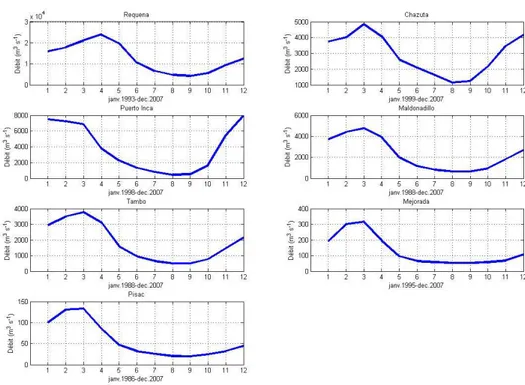
6

Liste des Tableaux

Tableau I-1. Classifications des climats d’après Thornthwaite, 1948a.Voir Figure I-2. ... 10 Tableau II-1. Typologie de sols. D’après FAO/UNESCO, 1981. ... 40 Tableau II-2. Sous bassins sélectionnés sur les bassins des rios Ucayali et Huallaga. Ar. Dr. est la superficie drainée, et période est la période de données de débits disponibles pour chaque station. ... 45 Tableau II-3. Classification des sols selon la capacité de rétention en eau en mm (d’après FAO/UNESCO, 1981) ... 69 Tableau II-4. Valeurs obtenues pour estimer la capacité de rétention en eau pour l’unité de sol Qa5-1a. ... 70

(15)

CHAPITRE 1

(16)

CHAPITRE 1. Introduction 8

I. CHAPITRE 1. Introduction

rès peu d’études hydrométéorologiques exhaustives ont été à l’heure actuelle menées sur le Pérou. Les études précédentes sont en général très localisées sur des régions spécifiques et se basent sur des données climatologiques parcellaires (par exemple Gentry et Lopez-Parodi, 1980 ; Rocha et al., 1989 ; Marengo, 1995; Marengo et al., 1998a ; Rome-Gaspaldy et Ronchail, 1998 et autres). Récemment, la fonte des glaciers péruvien qui incluent 71% des glaciers tropicaux est devenu un enjeu qui rentre dans le cadre plus général de la mise en évidence d’un réchauffement global (Pouyaud et al., 2005). Ces études d’impact sur la ressource en eau ont porté spécifiquement sur le bassin du Rio Santa situé sur le versant Pacifique (Pouyaud et al., 2005 et Kaser et al., 2003). La deuxième problématique concerne le bassin Amazonien, d’une superficie de 6 000 000 km2 avec un débit moyen annuel de 209 000 m3

1.1 Contexte général du Pérou

/s (Molinier et al., 1996), qui se caractérise récemment par des événements extrêmes tels que la sécheresse de 2005 et la crue historique de 2009. Au Pérou, le Bassin Amazonien (BA) couvre 74.5% du territoire péruvien et fait actuellement l’objet d’une déforestation rapide (Oliveira et al., 2007), entraînant des crues importantes dans les zones de piémont. Le BA au Pérou se caractérise par la présence de régions de hautes altitudes couplées à de fortes pentes (les Andes) et de régions de plaines (la Forêt). Les rivières dans les Andes sont utilisées pour des usages agricoles, domestiques et énergétiques, tandis que dans la plaine amazonienne les fleuves sont utilisés comme moyen de communication entre les villages. Pour ces raisons, nous nous proposons de préciser les processus hydrologiques impactant le BA péruvien, ainsi que d’évaluer les impacts du changement climatique sur les régimes hydrologiques.

Le Pérou (1 285 220 Km2 Figure I-1

) est un pays caractérisé par divers ensembles physiographiques ( ) et climatologiques (Figure I-2). Pulgar (1941) a proposé de grouper les différences altitudinales en 8 régions homogènes : Chala ou Costa (0 à 500 m.s.n.m.), Yunga (500 à 2300 m.s.n.m.), Quechua (2300 à 3500 m.s.n.m.), Suni ou Jalca (3500 à 4000 m.s.n.m.), Puna (4000 à 4800 m.s.n.m.), Janca ou Cordillera (4800 à 6768 m.s.n.m.), Rupa rupa ou Selva Alta (400 à 1000 m.s.n.m.) et Omagua ou Selva Baja (80 à 400 m.s.n.m.). Cette classification a été reprise par le SENAMHI (2005) en utilisant la classification climatique de Thornthwaite (Thornthwaite, 1948a), mettant ainsi en évidence 27 zones climatiques différentes au Pérou (voir Figure I-2 et Tableau I-1). Voici les caractéristiques de ces différentes zones :

- Climat Semi - Chaud Très Sec (Désertique-Aride-Sous Tropical) : ce type

de climat constitue un ensemble climatique remarquable sur le Pérou et s’étend sur presque toute la région de la côte, depuis Piura jusqu'à Tacna et depuis le littoral Pacifique jusqu'à l’altitude de 2000 m.s.n.m. environ, et représente 14% de la surface totale du pays. Ce climat se distingue par une précipitation moyenne annuelle 150 mm, une température moyenne annuelle de 18° à 19°C qui diminue dans les zones les plus élevées de la région.

- Climat Chaud Très Sec (Désertique ou Aride Tropical) : Il comprend le secteur septentrional de la région côtière, qui inclut une grande partie des départements de Tumbes et Piura, entre le littoral marin et la côte approximativement jusqu'à 1000 m.s.n.m. Il représente moins de 3% (35 000 km2

T

) de la surface du pays. Ce climat est très sec et chaud, avec une précipitation moyenne annuelle autour de 200 mm et une température moyenne annuelle de 24.7°C, sans changement thermique hivernal défini.

(17)

Figure I-1. Gauche : relief du Pérou en altitudes (http://geografia.laguia2000.com). Droite : république du Pérou en Amérique du Sud au 1er janvier 2009 (http://fr.wikipedia.org/wiki/fichier:south_america_location_per.png).

- Climat Semi - Chaud Très Sec (Désertique-Aride-Sous Tropical) : ce type

de climat constitue un ensemble climatique remarquable sur le Pérou et s’étend sur presque toute la région de la côte, depuis Piura jusqu'à Tacna et depuis le littoral Pacifique jusqu'à l’altitude de 2000 m.s.n.m. environ, et représente 14% de la surface totale du pays. Ce climat se distingue par une précipitation moyenne annuelle 150 mm, une température moyenne annuelle de 18° à 19°C qui diminue dans les zones les plus élevées de la région.

- Climat Chaud Très Sec (Désertique ou Aride Tropical) : Il comprend le secteur septentrional de la région côtière, qui inclut une grande partie des départements de Tumbes et Piura, entre le littoral marin et la côte approximativement jusqu'à 1000 m.s.n.m. Il représente moins de 3% (35 000 km2

- Climat Tempéré Subhumide (Steppe et Faibles Vallées Interandines) : ce

climat est propre à la région de montagne, correspondant aux vallées Interandines, d’altitude faible et intermédiaire, situées entre 1000 et 3000 m.s.n.m. Les températures dépassent les 20°C, et la précipitation moyenne annuelle est inférieure à 500 mm mais peut dépasser 1200 mm/an dans les parties les plus humides et orientales.

) de la surface du pays. Ce climat est très sec et chaud, avec une précipitation moyenne annuelle autour de 200 mm et une température moyenne annuelle de 24.7°C, sans changement thermique hivernal défini.

- Climat Boréal (des Vallées Mesoandines) : Ce climat s’étend sur la région de

montagne entre 3000 et 4000 m.s.n.m. Il se caractérise par des précipitations annuelles de l’ordre de 700 mm et des températures moyennes annuelles de l’ordre de 12°C. Les étés sont pluvieux et les hivers secs avec de fortes gelées.

(18)

Figure I-2. Classification climatique du Pérou en utilisant la classification de Thornthwaite (d’après SENAMHI, 2005. Voir Tableau I-1).

Tableau I-1. Classifications des climats d’après Thornthwaite, 1948a.Voir Figure I-2.

Climats

Pluie effective Efficience de température

A Très pluvieuse A' Chaud B Pluvieuse B'1 Semi-chaud C Semi-sec B'2 Tempéré D Semi-aride B'3 Semi-frais E Aride C' Frais D' Semi-froid E' Froid F' Polaire

Distribution de la pluie dans l'année Humidité Atmosphérique r Pluvieux pendant toutes les saisons

i Hiver sec H1 Très sec

p Printemps sec H2 Sec

v Été sec H3 Humide

o Automne sec H4 Très humide

(19)

CHAPITRE 1. Introduction 11 - Climat Froid (de Toundra) : Ce type de climat, connu comme climat de Puna, correspond aux secteurs les plus élevés de la région andine compris entre 4000 et 5000 m.s.n.m. Il couvre environ 13% du territoire péruvien (170 000 km2

- Climat de Neige (Gélido) : Ce climat correspond aux zones des neiges éternelles, avec des températures moyennes pendant tous les mois de l'année sous le point de congélation (0°C). Il est situé dans les secteurs dont l’altitude dépasse 5000 m.s.n.m. et qui sont recouvert par de grandes quantités de neige et de glace.

). Il se caractérise par des précipitations annuelles moyennes de 700 mm et températures moyennes annuelles de 6°C. Il comprend les collines, plateaux et sommets andins. Les étés sont toujours pluvieux et nuageux ; et les hivers (juin-août), sont extrêmes et secs.

- Climat Semi - Chaud Très Humide (Subtropical très Humide) : Ce type de climat prédomine dans la forêt. Il se caractérise par son haut degré d’hygrométrie, avec des précipitations dépassant 2 000 mm/an et des valeurs extrêmes supérieures à 5 000 mm/an par exemple dans la région de Quincemil. Les températures sont inférieures à 22°C en général mais des températures plus élevées sont enregistrées dans les fonds des vallées et dans les zones de transition vers la plaine Amazonienne. - Climat Chaud Humide (Tropical Humide) : Ce climat correspond aux plaines amazoniennes péruviennes. Il se caractérise par des précipitations moyennes annuelles de l’ordre de 2 000 mm et une température moyenne supérieure à 25°C, sans changement bien défini entre les saisons.

En conclusion, la présence de la Cordillère des Andes et de l’Altiplano divise les réseaux de drainage en trois bassins versants : Pacifique, Lac Titicaca et Amazonas (Atlantique) (Figure I-3). D’après un rapport de l’ UNESCO (2006), la distribution moyenne annuelle du bilan hydrique (ruissellement) pour la période 1969-1999, calculée par différence entre les précipitations et l’évapotranspiration est de 16.4 mm sur le versant Pacifique, 129.8 mm sur le bassin du Lac Titicaca et 2696.5 mm sur le versant Amazonien. Ainsi, le ruissellement estimé par UNESCO (2006) est en opposition avec la distribution de la population au Pérou, où les plus grandes villes (Lima, Arequipa et Piura) sont situées sur le versant Pacifique.

1.2 A basin-scale trends in rainfall and runoff in Peru (1969-2004): Pacific, Titicaca and Amazonas drainage.

WALDO SVEN LAVADO CASIMIRO, JOSYANE RONCHAIL, DAVID LABAT,

Cette section de la thèse sera présentée via un article en préparation. Il a été décidé de rajouter cette partie au document final car elle présente une vision globale et intégratrice du problème de la ressource en eau au Pérou.

JHAN CARLO ESPINOZA & JEAN LOUP GUYOT

(20)

Figure I-3. Versants du Pérou : Versant du Pacifique (ouest), Versant du Lac Titicaca (sud est) et Versant de l’Amazonas (est). (D'après UNESCO, 2006).

Résumé

Cette étude, basée sur des données s’étendant de 1969 à 2004, propose pour la première fois une analyse exhaustive des tendances hydroclimatologiques au Pérou. Cette contribution porte sur les trois principaux bassins versants du Pérou : Pacifique, Lac Titicaca et Amazonas, et porte sur les débits maxima (Qmax), moyens (Qmean) et minima (Qmin). Au total, une trentaine de bassins versants ont été étudiés : 29 dans la zone Pacifique, 3 dans la zone du Lac Tititcaca et 2 bassins versants (5 pour les pluies) dans la zone Amazonienne.

Les débits minima sont caractérisés en général par une tendance positive alors que cette tendance est négative sur la zone Pacifique. En effet, la plupart des bassins du nord de la zone

(21)

CHAPITRE 1. Introduction 13 Pacifique sont caractérisés par des tendances négatives pouvant être reliées à la croissance des surfaces agricoles, et donc des besoins en eaux pour l’irrigation. Les débits minima mesurés dans les bassins des rios Chillon et Rimac présentent des tendances positives. En effet, ces ressources sont dédiées à un usage domestique, en particulier pour la population de la ville de Lima, capitale du Pérou. Des tendances opposées dans les débits minima observées dans la partie Sud de la zone Pacifique sont aussi imputables aux usages agricoles de l’eau. Enfin, les séries pluri-annuelles de Qmax, Qmean, Qmin et de précipitations mesurées sur la zone Pacifique sont comparées avec les principaux indices de circulation générale : L’index d’Oscillation du Sud (SOI), les températures superficielles de la mer (SST) dans l’Atlantique nord (NATL SST) et les différences des NATL moins la SST dans l’Atlantique Sud (SATL).

SUMMARY

According to the Peruvian Agricultural Ministry, the Pacific watersheds, where are located great cities and intense farming, only benefit from 1% of the available fresh water in Peru. That is why a thoroughfull knowledge of the hydrology of this region is of particular importance. In this study, it is completed by the analysis of the two other main Peruvian drainages, the Altiplano and the Amazon. Rainfall and runoff data collected by the National Service of Meteorology an Hydrology (SENAMHI) and controlled in the mark of the Hydrogeodynamics of the Amazon basin (HYBAM) program is the basis of this basin scale study that involve the 1969-2004 period. On the cost, runoff changes (increases or decreases) are detected during the low stage season. They mainly depend on human activities and infrastructures aimed at cities supplying and increasing agricultural exports that may remove water or on the contrary help sustain the minimum runoff. In the Amazon basin, natural causes as the long term warming of the northern tropical Atlantic explain the runoff diminution since the middle of the eighties.

Keywords: trend, rainfall, runoff, climate variability, Titicaca basin, Amazon, Pacific coast, Peru, tropical Atlantic.

INTRODUCTION

The North-South Andes cordillera in Peru (1 285 216 km2) determines the presence of three main drainage basins (Figure 1), one toward the Pacific Ocean (Pd) on the western side of the Andes, another toward the Amazon basin on the eastern side on the Cordillera (Ad ) and the southern endorheic Titicaca Lake basin on the Altiplano (Td ). The Peruvian National Water Agency reports that Pd, Td and Ad represent respectively 21,7%, 3,8% and 74,5% of Peru and include 62, 13 and 84 main basins, respectively (Ruiz et al., 2008). The multi-annual water balance (difference between rainfall and evapotranspiration) has been computed for the 1969-1999 period by UNESCO (2006). It results that the available superficial water is 16.4 mm in Pd, 129.8 mm in Td and 2696.6 mm in Ad. Unfortunately, the availability of fresh water resources in Peru is opposite to population density, given that 88% of the population lives in along the Pacific coast, around the Titicaca lake and in the Andean zones of the Amazon basin, where there are only 2% of the Peruvian fresh water resources. Indeed, the greatest Peruvian cities (i.e. Lima, Arequipa and Piura) are in Pd where there is only 0.6% of the available fresh water of Peru. According to the Agricultural Minister (www.minag.gob.pe) Pd is an arid but fertile land. Agriculture has been developed thanks to irrigation that uses about 80% of the available water while domestic usages consume about 12% of the Pd available water. Private and public investments have been gathered in order to develop these infrastructures aimed at increasing agricultural exports.

Pd features small size basins with rivers initiating in the Andes cordillera and presenting a west to east direction, from the Andes toward the Pacific Ocean (Figure 1). These basins

(22)

CHAPITRE 1. Introduction 14 exhibit bare and steep slopes that favour an important erosion and floods during the rainy season. Td is located on the Altiplano (Southeast of Peru) and its endorheic drainage is realized toward Titicaca lake (~ 3800 m a.s.l.), then Desaguadero river and finally Poopo and Salar de Coipasa lakes in Bolivia. The Ad is characterized by hot tropical lowlands near sea level and freezing cold tropical high mountain peaking at up to 6000 m a.s.l. of elevation;

Figure 1. A) Elevation of the zone of study, mains rivers et limits of the selected basins. (see Table 1). B) Location of the zone of study in South America. C) Location of the rainfall gauges used in this study.

seldom in the world are such dramatic environmental contrasts lying closer together. Naturally, each of these two realms is subject to different, but in many aspects interrelated, sets of physical, geochemical and biologic parameters (ACTO, 2005). The rivers in the Ad exhibit steep slopes in the Andean western region while they are very smooth in the flat eastern lowlands.

Peruvian hydroclimatology is influenced by the disruption of the large-scale circulation patterns caused by the Andes cordillera, the contrasting oceanic boundary conditions and the landmass distribution (Garreaud et al., 2008). Low rainfall in Pd region is explained by the strong, large scale subsidence over the south-eastern subtropical Pacific Ocean and the southern Pd exhibits conditions of extreme aridity due to regional factors (Rutllant et al., 2003). Annual rainfall increases toward North in accordance with the seasonal southward displacement of the Pacific Intertropical Convergence Zone (ITCZ). UNESCO (2006) assesses that mean rainfall and runoff in Pd are about 274.3 mm and 168.1 mm respectively during the 1969-1999 period. Santa basin is an exception along the Pacific coast (PQ-10, Figure 1 and Table 1) as its water level is influenced by the melting of an upstream 600 km2 glacier (Georges, 2004).

(23)

CHAPITRE 1. Introduction 15 Table 1 Gauging stations used in this study. Lat. is latitude; Long. is longitude; Alt. is altitude and Dr. Ar. is Drainage Area

Gauging station River Code Lat. _Long. Alt. (m l ) Dr.Ar. (Km2) El Tigre Tumbes PQ-1 3.72°S 80.47°W 40 4802 El Ciruelo Chira PQ-2 4.30°S 80.15°W 250 7760 Pte. Ñacara Piura PQ-3 5.11°S 80.17°W 119 4765 Racarumi Chancay-Lambayeque PQ-4 6.63°S 79.32°W 250 2401 Batan Zaña PQ-5 6.80°S 79.29°W 260 681 Yonan Jequetepeque PQ-6 7.25°S 79.10°W 428 3354 Salinar Chicama PQ-7 7.67°S 78.97°W 350 3651 Quirihuac Moche PQ-8 8.08°S 78.87°W 200 1918 Huacapongo Viru PQ-9 8.38°S 78.67°W 280 941

Pte. Carretera Santa PQ-10 8.97°S 78.63°W 18 11869 Yanapampa Pativilca PQ-11 10.67°S 77.58°W 800 4270

Sayan Huaura PQ-12 11.12°S 77.18°W 650 2896

Santo Domingo Chancay-Huaral PQ-13 11.38°S 77.05°W 697 1881 Larancocha Chillon PQ-14 11.68°S 76.80°W 120 1238

Chosica Rimac PQ-15 11.93°S 76.69°W 906 2339

La Capilla Mala PQ-16 12.52°S 76.50°W 424 2141

Socsi Cañete PQ-17 13.03°S 76.20°W 330 6003

Conta San juan PQ-18 13.45°S 75.98°W 350 3144 Letrayoc Pisco PQ-19 13.65°S 75.72°W 720 3107 Los Molinos Ica PQ-20 13.92°S 75.67°W 460 2154 Bella Union Acari PQ-21 15.48°S 74.63°W 70 4369 Puente Jaqui Yauca PQ-22 15.48°S 74.45°W 214 4245 Pte. Ocoña Ocoña PQ-23 16.42°S 73.12°W 122 16646

Huatiapa Majes PQ-24 16.00°S 72.47°W 699 13651

Pte. Del Diablo Chili PQ-25 16.41°S 71.50°W 236 8750 La Pascana Tambo PQ-26 16.99°S 71.64°W 281 12884 Pte. Viejo Locumba PQ-27 17.62°S 70.77°W 550 3639 La Tranca Sama PQ-28 17.73°S 70.48°W 620 1993 Aguas Calientes Caplina PQ-29 17.85°S 70.12°W 130 569 Pte. Ramis Ramis TQ-1 15.26°S 69.87°W 385 16229 Pte. Huancane Huancane TQ-2 15.22°S 69.79°W 386 3714 Pte. Ilave Ilave TQ-3 16.09°S 69.63°W 385 8714 Tabatinga Amazonas AQ-1 4.25°S 69.93°W 60 890308 Tamshiyacu Amazonas AQ-2 4.00°S 73.16°W 105 733596 San Regis Marañon AQ-3 4.51°S 73.95°W 80 359910

Borja Marañon AQ-4 4.47°S 77.55°W 450 115478

Requena Ucayali AQ-5 5.03°S 73.83°W 200 354316

On the contrary, very wet conditions are observed in the Amazon basin, on the eastern side of the Andes, due to the convection of moist and hot air that originates in the evapotranspiration of the rainforest and in the humid air advection from the tropical Atlantic. According to UNESCO (2006), mean rainfall over Ad during the 1969-1999 period is close to 2060 mm. But very high and low rainfall values (between 6000 and 250 mm/year) can be observed in nearby stations due to the leeward or windward position of rain gauges (Espinoza et al., 2009b). More, annual rainfall tends to diminish with altitude, being under 1500 mm above 2000 m.a.s.l. (Espinoza et al., 2009b). UNESCO (2006) estimates that on the Altiplano mean annual rainfall and runoff during the 1969-1999 period are 813.5 mm and 89 mm,

(24)

CHAPITRE 1. Introduction 16 respectively. In this region, water vapour originates in the Amazon basin (Vuille et al., 1998; Chaffaut et al., 1998; Garreaud, 1999; Garreaud et al., 2003; Vizy et Cook, 2007) and it is locally enhanced around the Titicaca Lake (Roche et al., 1990).

In northern Pd and Td rainfall and runoff interannual variability are oppositely influenced by El Niño Southern Oscillation (ENSO). During El Nino, rainfall and runoff are higher than normal in Pd while there is an hydrologic drought in Td and over the high slopes of the Amazon basin (Waylen et Caviedes, 1986; Aceituno, 1988;Ropelewski et Halpert, 1987; Tapley et Waylen, 1989; Tapley et Waylen, 1990 ; Rome-Gaspaldy et Ronchail, 1998; Vuille et al., 2000;Waylen et Poveda, 2002; Espinoza et al., 2009b ; Romero et al., 2007, among others). Moreover, interannual rainfall variability in Southern Ad is indirectly related to the North Atlantic sea surface temperatures (NATL SSTs) (Lavado et al., Submitted-b) as well as runoff in the Amazonian basin, Tamshiyacu (AQ-2, Table 1; Espinoza et al., 2009a).

Long term rainfall and runoff variability has also been described in Peru. Marengo (1995) and Marengo et al., find decreasing runoff trends during the twentieth century in some gauging stations located in the northern Pd. They are often related to water catchment for irrigation and domestic usage in growing cities and farming zones. Also, Santa basin is in process of glacier retreat and lost mass (Kaser et al 2003, Mark et Seltzer, 2005; Pouyaud et al., 2005; Vuille et al., 2008a;Vuille et al., 2008b; among others), they have added to a temporary increase in runoff (Mark et Seltzer, 2005; Vuille et al., 2008a). On the Altiplano, a 13 years climatic period is observed in Quelccaya ice-cores (Melice et Roucou, 1998) and a recent decrease (since the end of the eighties) is detected in the level of Titicaca Lake that acts as a rainfall gauge for the Td region (Rigsby et al., 2003). In the Ad, Gentry et Lopez-Parodi (1980) associated upward (downward) trends in maximum (minimum) water levels in Iquitos (AQ-2, see Table 1) during the 1962-1978 period with deforestation as no clear rainfall change had been observed during the same period. Nordin et al.(1982) and Richey et al. (1989) discussed these results as well as Rocha et al. (1989) who find positive rainfall trends in Iquitos and Pucallpa stations during the 1955-1979 and 1957-1981 period respectively. On the contrary and more recently, Haylock et al.(2006) find a downward rainfall trend during the 1957-1994 period showing that the sign of long term variation changes with time. Marengo (2004) and Espinoza et al. (2006a; 2009a; 2009b) confirm this observation and propose a space variation of long term changes also within the Amazon basin, especially between the North and the South. Espinoza et al. (2007) describe upward runoff trends in the northern Ad (AQ-3, Table 2), whereas downward runoff trend over the southern Ad (AQ-5, Table 2) during the 1990-2005 period.

The studies mentioned above often involve a particular region of Peru and use few stations. That is why the aim of this study is to gather a comprehensive set of rainfall and runoff data in all the whole Peruvian territory (Pacific, Amazonas and Titicaca drainage) in order to propose, for the first time, a global outline about its mean hydrological characteristics and about its recent variability. This was made possible thanks to the collection, the validation and the completion of information through runoff gauging in big rivers of the Peruvian Amazon, in the mark of the Hydrogeodynamics of the Amazon Basin (Hybam) project that associate the Peruvian National Meteorology and Hydrology Service, SENAMHI (www.senamhi.gob.pe) and the French Institute for Reseach and Development (IRD).

This paper is organized as follow. After the introduction, the database and the methods used in this paper are described. The spatial distribution of rainfall and discharge and their annual cycles in the different basins are depicted. The relationship between annual rainfall and discharge is discussed and their interannual variability is addressed. We then comment on trends and breaks in discharge and annual series. Finally, hydrological variability is related to regional ocean-atmospheric indicators. A summary and concluding remark are provided in the

(25)

CHAPITRE 1. Introduction 17 last section.

DATA AND METHODS

This work is based on monthly rainfall and discharge data in 33 basins (29 in Pd, 3 in Td and 2 in Ad), during the 1969/70 - 2003/04 period, with an hydrological year running from September to August (Table 1, Figure 1). Basins subdivision was made using the Digital Elevation Model (DEM) provided by the National Aeronautics and Space Administration, NASA through the Shuttle Radar Topography Mission, SRTM (www2.jpl.nasa.gov/srtm). The SRTM data is available as 3 arc second (~ 90m resolution), a description of this model is given by Farr et al. (2007).

Although being the largest part of the country, Ad holds a very small number of stations because measures generally began recently, during the eighties. In Ad long times series have been obtained in very large basins that almost reach 1 million km². On the contrary, basins in Pd and Td are more numerous and small, not surpassing 20 000km².

Monthly runoff data is from the SENAMHI and from the National Water Agency from Brazil (ANA, www.ana.gov.br) for the station of Tabatinga (AQ-1). Homogenisation was performed by SENAMHI using double-cumulative techniques. Cross correlations between all stations were calculated and missing data periods were filled using linear regression with nearby stations showing the highest correlation, always significant at the 99% level.

Monthly rainfall data from 1965 to 2007 are from the SENAMHI network and have been criticized by this institute. Pd and Td data (119 stations) have been already documented by UNESCO (2006), for the 1969-1999 period. In the mark of the Hybam program, rainfall data over Ad (48 stations) were preliminary controlled by Espinoza et al. (2009b) for the 1965-2003 period and by Lavado et al. (Submitted-b) for the 1965-2003-2007 period. Both studies used the Regional Vector Method – RVM (Hiez, 1977 and Brunet-Moret, 1979),.

Rainfall stations are more abundant in Pd and Td than in Ad where they are concentrated in the Andes head basins that are more easily reached than the lowlands. To measure the average rainfall in each basin, the Kriging interpolation method is applied (Oliver et Webster, 1990, Deutsch et Journel, 1992). This method consists in establishing a variogram for each spatial point. This variogram evaluates the influence of the 16 closest stations according to distance. The Kriging method is the only one that takes into consideration a possible spatial data gradient which is very important in a mountainous region.

Annual maximum and minimum runoff (Qmax and Qmin respectively) are individualized and complement the mean annual runoff (Qmean). They are the monthly runoff values of the months with the highest and lowest runoff values respectively.

Seasonal variation coefficients (sVC) are calculated using the mean monthly rainfall and runoff. Likewise, interannual variation coefficients (VC) are computed using annual rainfall and runoff values.

Two trend tests were used in this work to analyze temporal fluctuations in hydroclimatic series. The Bravais-Pearson coefficient which is parametric measures the lineal correlation among variables, whereas Mann-Kendal coefficients is non-parametric and based on range probability of the data occurrence order (Mann, 1945 and Kendall, 1975a). Mann-Kendal test is considered as an excellent tool for trend analysis in climatic series (Zhang et al., 2001, Burn et Elnur, 2002). An index for trend measure is calculated using Eq. 1, where b is the slope of the linear trend and X is the mean value in the series (Espinoza et al., 2009a).

(26)

Table 2. Average Characteristics of Hydrometeorology variables, using the hydrological year (from September to August) in each case, for the 1970-2004 period except PQ-10 with 1970-1999 period for runoff. P: Rainfall; Q: Runoff; CV: coefficient of variation; r: Linear correlation coefficient (Rainfall-Runoff). Significant values (95%): bold characters.* only rainfall analysis. ** Non-calculated.

Code P Q Q max. Q min. CV CV CV CV r CV

Seasonal (mm) (m3 s-1) (m3 s-1) (m3 s-1) (P) (Q) (Q max.) (Q min.) P Q PQ-1 917 114 371 15 0.4 0.6 0.5 0.3 0.77 0.8 1.0 PQ-2 1011 115 321 24 0.4 0.6 0.7 0.6 0.57 0.7 0.8 PQ-3 618 28 120 0 0.8 1.5 1.2 3.3 0.96 1.3 1.3 PQ-4 722 34 91 7 0.4 0.3 0.4 0.4 0.79 0.7 0.7 PQ-5 750 8 22 2 0.7 0.6 0.9 0.4 0.89 0.8 0.7 PQ-6 681 28 97 2 0.9 0.6 0.6 0.7 0.75 0.9 1.0 PQ-7 744 25 113 2 0.4 1.0 1.1 0.8 0.93 0.9 1.2 PQ-8 517 9 35 0 0.4 0.9 1.1 1.2 0.90 0.9 1.1 PQ-9 583 4 19 0 0.4 1.3 1.3 1.2 0.68 0.7 1.4 PQ-10 489 201 550 49 0.2 0.4 0.4 0.3 0.36 0.7 0.7 PQ-11 521 43 115 12 0.3 0.3 0.4 0.5 0.59 0.9 0.6 PQ-12 493 29 85 10 0.3 0.4 0.6 0.3 0.61 0.9 0.8 PQ-13 460 18 61 5 0.3 0.4 0.6 0.4 0.75 1.1 0.9 PQ-14 455 6 18 2 0.3 0.4 0.4 0.9 0.47 1.1 0.8 PQ-15 515 31 70 17 0.2 0.3 0.4 0.3 0.52 1.0 0.5 PQ-16 409 15 59 1 0.3 0.5 0.5 0.6 0.65 1.1 1.2 PQ-17 407 49 155 9 0.2 0.5 0.7 0.3 0.64 1.0 0.9 PQ-18 184 10 45 0 0.3 0.7 0.9 1.2 0.57 1.3 1.2 PQ-19 500 21 82 2 0.3 0.5 0.7 0.7 0.44 0.9 1.1 PQ-20 357 1 3 0 0.4 0.5 0.5 NC 0.43 1.1 1.4 PQ-21 240 14 72 0 0.4 0.8 0.8 3.0 0.49 1.1 1.5 PQ-22 237 9 45 0 0.4 0.8 0.9 0.4 0.50 1.3 1.4 PQ-23 487 71 244 17 0.3 0.5 0.5 0.6 0.50 1.1 0.9 PQ-24 463 86 291 26 0.3 0.3 0.4 0.2 0.75 1.1 0.9 PQ-25 305 13 45 6 0.3 0.7 1.0 0.6 0.64 1.2 0.7 PQ-26 281 28 90 11 0.4 0.6 1.0 0.5 0.62 1.3 0.7 PQ-27 230 3 5 2 0.4 0.2 0.5 0.3 0.40 1.4 0.3 PQ-28 164 3 12 1 0.5 0.6 0.7 1.0 0.82 1.5 1.2 PQ-29 144 1 2 0 0.5 0.3 0.6 0.3 0.65 1.4 0.5 TQ-1 773 76 260 8 0.2 0.3 0.3 0.4 0.82 0.9 1.1 TQ-2 729 20 78 2 0.2 0.4 0.5 0.5 0.86 0.8 1.1 TQ-3 620 39 172 5 0.2 0.5 0.6 0.5 0.78 0.9 1.2 AQ-1 1913 38044 53710 22545 0.1 0.1 0.1 0.2 0.82 0.2 0.3 AQ-2 1701 32605 49238 16603 0.1 0.1 0.1 0.2 0.60 0.2 0.3 AQ-3* 1747 0.1 0.5 AQ-4* 1463 0.1 0.3 AQ-5* 1496 0.1 0.2 100 × = X b Itrend (1)

In addition, Pettitt non-parametric test for mean-change measure in temporal hydrological annual series was applied (Pettitt, 1979). It is based on changes in the average and the range of the series subdivided into sub-series and it is considered as one of the most complete test

(27)

CHAPITRE 1. Introduction 19 to identify mean-change (Zbigniew et Robson, 2004). Significance level (a) is the probability that a test detects trend or other change when none is present (Robson et al., 2000). In this study, the null hypothesis in statistical tests is rejected using α equal 0.05 .

Several regional climatic indexes were used to characterize the time variability of rainfall and runoff. The Southern Oscillation Index (SOI) is the standardized pressure difference between Tahiti and Darwin. Monthly SSTs (1950–2000) are provided for the northern tropical Atlantic (NATL, 5–20°N, 60–30 °W) and the southern tropical Atlantic (SATL, 0–20 °S, 30 °W–10 °E). The standardized SST difference between the NATL and SATL is computed to feature the SST gradient in this oceanic basin. All these values are from the Climatic Prediction Centre of the National Oceanic and Atmospheric Administration (CPCNOAA:

http://www.cdc.noaa.gov/).

Finally, the management of the rainfall and runoff databases, as well as the calculation of the average rainfall in the basins, have been carried out using the HYDRACCESS software, developed within the framework of the HYBAM programme (free download at

www.mpl.ird.fr/hybam/outils/hydraccess en.htm; Vauchel, 2005b).

SPATIAL AND SEASONAL VARIABILITY OF RUNOFF AND RAINFALL

Mean annual rainfall values (1970-2005) in 167 stations, interpolated using the Kriging method, are displayed in Figure 2. A strong opposition appears between the rainy eastern lowlands in the Amazon basin (more than 1500 mm/year – see also Table 2) and drier conditions in the Andes and in the basins of the Pacific coast (less than 1000 mm/year). Weak rainfall along the Pacific coast is related to the subsidence in the South East Pacific subtropical anticyclone that prohibits rainfall. Though, in Pd, rainfall increases while latitude diminishes, from very low values in the southernmost basins (144 mm/year in PQ29, Table 2) to nearly 1000 mm/year in the North (Figure 3a). This can be related to the diminution of the strength of the southern Pacific anticyclone toward North and to the seasonal southward displacement of the Pacific ITCZ that reaches the northern coast of Peru. This South-North gradient is also observed in the specific runoff of the river (Figure 3b) that has been computed in order to avoid the problem of dependence between runoff and size of the basin. The specific runoff increases regularly toward North. More, along the Pacific coast rainfall increases with altitude with very low values near the coast (much lower than 100 mm/year in the South) and higher values in the higher parts of coastal basins, above the inversion layer that blocks the convection at about 500-800 meters (Dollfus, 1964 and Johnson, 1976). On the eastern flank of the Andes, on the contrary, rainfall is abundant. Though, local maximum and minimum are noticeable on Figure 1. In particular, very high annual rainfall (above 6000 mm/year) is recorded in regions where the concave form of the Andes favours convergence (Borja region) or in valleys opened toward North and oriented toward the humid north-western wind (High center Ucayali valley) (Figueroa et Nobre, 1990; Laraque et al., 2007; Espinoza et al., 2009b). They contrast with less rainy regions as the high Huallaga valley that is sheltered by relief and less exposed to moist air advection. Rainfall tends to increase when altitude diminishes as cool temperatures in the Andes do not favour a high moist content of the air.

(28)

Figure 2. Mean annual rainfall values (mm) for the 1965-2007 period over Pacific (Pd), Amazonas (Ad) and Titicaca (Td) drainages.

Figure 3. Relationship between latitude and mean multiannual A) specific runoff in Pacific drainage, B) rainfall. Labels and located of stations are described in Table 1.

(29)

CHAPITRE 1. Introduction 21 Monthly rainfall and runoff values expressed as a percentage of the hydrological annual values are represented in Figure 4 for some selected gauging stations. There is a pronounced annual cycle along the Pacific coast and in the Altiplano, with a rainy season during austral summer and a dry season in winter. The rainy season on the coast corresponds to the southward displacement of the Pacific ITCZ. The rainfall seasonal coefficient of variation are often higher than 0.7 (Table 2) and increase from the northern to the southern Pacific coast, revealing a higher seasonal variability in the South. Moreover, many rivers in Pd, in the North as well as in the South, are non permanent and are characterized by null or near null low-level flow in austral winter; this feature, consistent with the strong seasonality of rainfall, may explain the very high seasonal discharge coefficient of variation in some basins (Table 2). On the Altiplano, the rainy season in austral summer is characterized by an intense convective activity combined with moisture advection from the Amazon basin (Montecinos et Aceituno, 2003; Garreaud, 1999). During austral winter, the eastern moist flux is replaced by westerly winds, which provide dry air related to the atmospheric stability over the Pacific Ocean. Consequently the seasonal coefficients of variation of rainfall and discharge are about 1. In contrast, rainfall is abundant all year round in the Amazon basin, with a maximum in summer during the South American Monsoon (Zhou et Lau, 1998) and the seasonal coefficients of variation are much lower than in Pd and Td, i.e. 0,2 in AQ1 and AQ2 (Table 2).

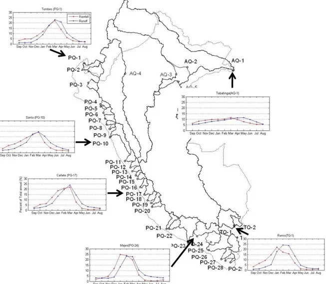
Figure 4. Mean monthly rainfall and runoff in percentage (ratio between monthly and mean annual values for runoff and ratio between monthly and total annual values for rainfall) in the selected basins in Peru.

(30)

CHAPITRE 1. Introduction 22 In the small northern and center and probably southern Pd basins (e.g. Tumbes PQ-1, Santa PQ-10 and Cañete PQ-17) there is an immediate runoff response to rainfall with discharge peaks in March and low values in austral winter. Santa basin (PQ-10) shows singular characteristics (more runoff than rainfall in autumn and winter months, see Figure 3) due to glacier contribution (Pouyaud et al., 2005). In Southern Pd, there is one month lag between peaks in rainfall (January) and peaks in runoff (February) (e.g.). In greater basins there may be a month lag between the maximum rainfall and the high flow runoff (as in Majes PQ-24) In Td, there is one month lag between rainfall (January) and runoff (February) peaks in the large Ramis basin (TQ-1). As the sizes of the Amazonas basins are huge, there are two months lag between peaks in rainfall (Mars) and runoff (May) as in Tabatinga gauging station (AQ-1) (Espinoza et al., 2006a).

INTERANNUAL VARIABILITY OF RAINFALL AND DISCHARGE

Annual hydrological runoff and rainfall during the 1970-2005 period are plotted in Figure 5 for the same stations than in Figure 4. On average, mean annual rainfall and runoff present similar variability and are significantly correlated (Table 2). In some coastal basins (PQ10, PQ14, PQ15, from PQ18 to PQ23, PQ27), the correlations are low. This is due to the presence of underground water that sustain low flow runoff, to the melting of glaciers in upstream valleys as in the case of the Santa River (PQ10), to barrages or water derivation (for irrigation or city water supply, as in the case of the Rimac basin (PQ15) that drives water towards the city of Lima. Moreover, Tumbes river (PQ-1) shows huge rainfall and runoff anomalies during the last two ENSO extreme events (1982-1983 and 1997-1998) (Figure 4). This results in high rainfall and runoff interannual coefficients of variation (Table 2). Though, Qmin interannual coefficients of variation that are generally higher than Qmax CVs, experience a large set of values, from 0,3 in some basins until 3 in PQ3 and PQ21.

Correlation between rainfall and runoff are generally good in the Altiplano and in the Amazonas where the rivers are not equipped by man, except in AQ2. Interannual rainfall and runoff coefficients of variation (CVs) are very low in the Ad (see Tabatinga in Figure 5), indicating a low interannual variability, while they are a little higher in the Altiplano (see Ramis in Figure 5 and Table 2).

In summary, the Pd shows more rainfall and runoff variations than Td and Ad at seasonal and interannual time scale. This is particularly visible in Figures 6a and 6c where interannual coefficients of variation (MACV) of runoff and rainfall respectively are plotted against seasonal coefficients (SVC). Td and Ad stations are located near the origin of the graph while Pd basins are located higher, but occupying a wide range of values. Figures 6b and 6d show the ratio MACV / SVC in runoff and rainfall in Pd versus latitude. An opposition is evidenced between northern and southern stations, the northern Pd basins showing the highest interannual variation in rainfall and runoff, when compared to seasonal variation, probably in relation with the strong hydrological impacts of El Nino events in the northern coast. Another set of basins in the southernmost coastal region experiences a strong interannual runoff variability that is not observed in rainfall.

(31)

Figure 5. Annual series (September-August) for distinct basins over Peruvian drainages: the black lines are the mean annual runoff, the blue lines blue are the total annual rainfall, the black dotted lines are the maximum runoff and the black dashed lines are teh minimum runoff. Values are standardized and are corrected by coefficient in order to avoid confusion between the different lines. The coefficients are 4 for maximum runoff, 0 for mean runoff and -4 for minimum runoff.

Figure 6. Relationship between multi-annual variation coefficients (MAVC) and the seasonal variation coefficients (SVC) in A) runoff and C) rainfall. Ratio between MAVC and SVC plotted in function of latitude in stations located in the Pacific drainage for B) runoff and D) rainfall. Circle black: stations located over Pacific drainage. Red plus sign: stations located over Amazonas drainage. Blue upward triangle: stations located over Titicaca drainage.

(32)

RUNOFF AND RAINFALL CHANGES AND TRENDS

The years of significant mean changes in runoff and rainfall in the Peruvian basins have been computed using Pettitt test. They are presented between parentheses in Table 3. Runoff and rainfall trend analysis have been computed using Bravais Pearson and Mann Kendal tests. For each basin, the best result between both methods is given in Table 3.

The main result is a change in all variables in the middle of the eighties in the two Amazonian basins, with rainfall and runoff decreases that have already been described by Espinoza et al. 2009. Itrend values, ratio between the slope of the linear trend and the mean value of the series, indicate that the stronger runoff decrease is observed in Tamshiyacu where there is no significant rainfall decrease, while in Tabatinga a moderate runoff decrease can be related with an important diminution of rainfall. In both stations the stronger runoff decrease is observed in minimum runoff.

In the Altiplano, on the contrary, there is an increase in minimum runoff. It is significant in the large Ramis basin (TQ-1), with a change in 1986, but it is not related to a change in annual rainfall. Is it associated with changes in winter rainfall that are not detected with our data and analysis.

Along the Pacific coast, the main changes and trends are observed in minimal runoff. The signals are different from a station to another and they are not related to change in annual rainfall. As there is no regional signal (the trends are as well positive or negative, the changes occur at very different dates, from the seventies until the late nineties), we can hypothesize that atmospheric circulation and rainfall do not originate these changes. On the contrary, they may be related to climatic change (glacier melting) or to constructions dedicated to sustain low flow when the trend is positive, and to the increase of water pumping installations for agriculture or city use, when the trend is negative. Positive trends are found in the Chillon (PQ-14), Rimac (PQ-15), Yauca (PQ-22) and Sama (PQ-28). The runoff of Chillon (PQ-14) and Rimac (PQ-15) rivers are mostly dedicated to urban use for the Lima city that according the last census 2007 from the National Institute of Statistic and Informatics from Peru, INEI (www.inei.gob.pe), bind 30.8% of total Peruvian population. Thus, the minimum runoff increase is due to runoff’s control in the high rainy zones of these basins, which involve many reservoirs systems and include water transfer from the Amazon basin. Negative trends are observed in rivers Viru (PQ-9), Pativilca (PQ-11), Huaura ( PQ-12), Acari ( PQ-21), Ocona (PQ-23). In these basins agricultural activity may limit low flow discharge by surface and underground water pumping that has considerably increased since the 1990s, according to the Peruvian Agriculture Ministry (www.minag.gob.pe).

There is no trend in the big Santa River (PQ-10); on the one hand it benefits from the melting of the White Cordillera glacier but, on another hand, its water is intensely exploited for export agriculture production.

(33)

Table 3 Years of change (YC), when the Pettit test is significant at the 95% level, are between parentheses. Statistical trends for runoff (maximum, mean and minimum) and rainfall annual series (1970-2004 period except PQ-10 with 1970-1999 period for runoff). There is a trend if p<0.05, using the higher p value when using the linear Bravais-Pearson and the Mann-Kendall tests NEG. underlined values indicate significant negative trends (with 0>p>-0.05) and POS. bold values indicate positive significant trends ( with 0<p<0.05). nt is for “no trend”. Itrend is the ratio between the slope of the linear trend and the mean value of the serie. ** indicates that the trend has not been computed.

Code Maximum Runoff Mean Runoff Minimum Runoff Rainfall

TREND/YC Itrend TREND/YC Itrend TREND/YC Itrend TREND/YC Itrend

PQ-1 nt -0.218 nt 0.126 nt 0.494 nt 0.15 PQ-2 nt 0.422 nt -0.584 nt -1.525 nt 0.13 PQ-3 nt 2.464 nt 2.844 nt(1991) 2.105 nt 0.952 PQ-4 nt -0.626 nt -0.284 NEG.(1990) -2.344 nt 1.082 PQ-5 nt -0.151 nt -0.082 NEG. -1.687 nt 1.105 PQ-6 nt 0.692 nt 0.432 nt -1.593 nt(1991) 1.7 PQ-7 nt -0.071 nt 0.462 nt -1.84 nt 0.237 PQ-8 nt 0.893 nt 1.409 nt 2.533 nt 0.816 PQ-9 nt -0.975 nt -0.324 NEG.(1976) -5.738 nt -0.518 PQ-10 nt (1989) -1.756 nt -0.323 nt 0.605 nt -0.598 PQ-11 nt 1.113 nt -0.009 NEG.(1980) -2.232 nt -0.529 PQ-12 nt -1.622 nt -0.893 NEG.(1988) -1.56 NEG. PQ-13 -1.496 nt -1.77 nt -0.893 nt(1988) -1.18 nt -0.184 PQ-14 nt -0.953 nt 0.718 POS.(1994) 4.59 nt -0.956 PQ-15 nt -1.008 nt 0.447 POS.(1994) 1.479 NEG. PQ-16 -0.904 NEG. -1.956 nt -0.662 nt -0.543 nt(1992) 1.43 PQ-17 nt -2.357 nt -0.962 nt -0.128 nt 0.614 PQ-18 nt (1976) -4.349 nt -1.622 nt -1.601 nt 0.211 PQ-19 nt(1988) -2.262 nt -0.438 POS.(1991) 4.754 nt(1992) 1.409 PQ-20 NEG. -2.148 nt -0.828 ** ** nt 0.189 PQ-21 nt -0.4 nt 1.193 NEG.(1982) -11.922 POS.(1992) 2.688 PQ-22 nt -0.097 nt 1.287 POS.(1986) 2.031 nt PQ-23 0.476 nt -0.51 nt -1.1 NEG.(1989) -3.921 nt PQ-24 0.688 nt -0.926 nt -0.553 nt -0.487 nt PQ-25 0.41 nt 1.548 nt 1.102 nt 2.155 nt PQ-26 0.271 nt 1.738 nt 0.975 nt -0.206 nt PQ-27 -0.407 nt 0.911 nt -0.398 nt 0.061 nt PQ-28 -0.737 nt -0.641 nt -0.588 POS.(1997) 5.159 nt PQ-29 0.126 nt 1.722 nt 0.795 nt 0.124 nt TQ-1 -0.15 nt -0.671 nt -0.141 POS.(1986) 1.646 nt -0.102 TQ-2 nt -0.574 nt -0.023 nt 1.454 nt TQ-3 0.143 nt -1.033 nt -1.203 nt 0.712 nt AQ-1 -0.216 NEG.(1984) -0.488 NEG.(1984) -0.53 NEG.(1987) -1.166 NEG.(1984) -0.418

AQ-2 NEG.(1984) -0.792 NEG.(1987) -0.847 NEG.(1987) -1.544 nt(1978) -0.162

AQ-3 nt -0.168

AQ-4 nt -0.165

(34)

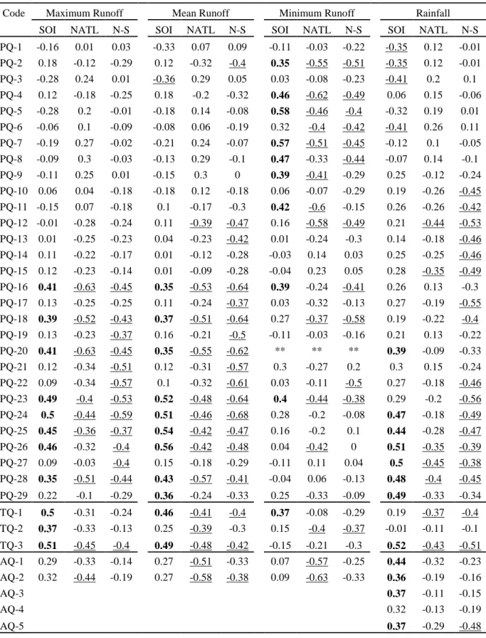
IMPACT OF OCEAN-ATMOSPHERIC INDICES ON PERUVIAN HYDROLOGY

In order to search explanation for the interannual and long term variability of runoff and rainfall, the hydrological series have been correlated to ocean-atmosphere indices as the Southern Oscillation Index (SOI) and Atlantic indexes constructed using Sea Surface Temperature (SST) in the southern and northern tropical Atlantic ocean. These indexes have been chosen because on the one hand coastal Peru is a key region for the El Nino – Southern Oscillation (ENSO) phenomena and because the tropical Atlantic SST is related to the strength of the trade winds and consequently to the water vapour advection from the Atlantic to the South America tropics (Marengo 1992, Marengo 2004). Their time series are presented in Figure 7a, b, c.

Figure 7. Standardized annual values (1969-2004 period) for A) the Southern Oscillation Index (SOI), B) the Northern tropical Atlantic SST (NATL, 5–20°N, 60–30 °W). C) the standardized difference between NATL and the southern tropical Atlantic SST (0–20 °S, 30 °W–10 °E), NATL-SATL. D) Interpolated correlation coefficients values in Ucayali and Huallaga basins. Stations with significant negative correlation between rainfall and NATL-SATL are represented by black downward triangles (95% of confidence level). Adapted from Lavado

et al.(Submitted-b).

Correlations values using Bravais Pearson test are reported in Table 4. They are very similar to those computed using Mann-Kendall test (not shown). Correlation values are often low, explaining generally 25 to 30% of the hydrological series variability. But in some cases the relationship is much higher and half of the variance may be represented.

In the Amazon basin, there is a large discrepancy between runoff and rainfall results. Rainfall is positively related to SOI, with less rain during El Nino while there is no runoff-SOI signal. On the contrary, there is a negative signal between NATL and runoff indicating a higher runoff when the northern Atlantic SST is cooler than usual and no signal in rainfall. This discrepancy may be due to the rainfall gauge stations sampling that has been used to compute rainfall in the Amazon basin. Many stations were available in the Andes while few stations in the lowlands that represent the largest and rainiest part of the basins. Consequently, rainfall mainly represents the tropical Andes, while runoff the lowlands. That is why an Andean usual