HAL Id: tel-03168172
https://pastel.archives-ouvertes.fr/tel-03168172
Submitted on 12 Mar 2021HAL is a multi-disciplinary open access archive for the deposit and dissemination of sci-entific research documents, whether they are pub-lished or not. The documents may come from teaching and research institutions in France or abroad, or from public or private research centers.
L’archive ouverte pluridisciplinaire HAL, est destinée au dépôt et à la diffusion de documents scientifiques de niveau recherche, publiés ou non, émanant des établissements d’enseignement et de recherche français ou étrangers, des laboratoires publics ou privés.
Aldo Serafino
To cite this version:
Aldo Serafino. Multi-fidelity Robust Design Optimization Methods for Organic Rankine Cycles. Me-chanics of the fluids [physics.class-ph]. HESAM Université, 2020. English. �NNT : 2020HESAE055�. �tel-03168172�
TH`
ESE
pr´esent´ee par :
Aldo SERAFINO
soutenue le :03 d´
ecembre 2020
pour obtenir le grade de :
Docteur d’HESAM Universit´
e
pr´epar´ee `a :Ecole Nationale Sup´
´
erieure d’Arts et M´
etiers
Sp´ecialit´e : G´enie m´ecanique
Multi-fidelity Robust Design Optimization Methods for
Organic Rankine Cycles
TH`ESE dirig´ee par: Mme CINNELLA Paola
Encadrant industriel: M. OBERT Benoˆıt
Jury
M. Vincent LEMORT Professeur, En. Sys. Lab., Universit´e de Li`ege Pr´esident
M. Didier LUCOR Directeur de recherche, DATAFLOT, LIMSI Rapporteur
M. Giacomo B.A. PERSICO Professeur, LFM, Politecnico di Milano Rapporteur
Mme. Paola CINNELLA Professeur, DynFluid, ENSAM Examinatrice
M. St´ephane CL´ENET Professeur, L2EP, ENSAM Examinateur
I wish to express my sincere gratitude and appreciation to Prof. Paola Cinnella for her guidance, patience and encouragement throughout the development of this project.
This PhD would not have been feasible without the engagement of ENERTIME and the French organisation for research and technology ANRT.
I want to thank Mr. Benoit Obert, for having followed me with passion until the conclusion of this project, and all the other colleagues of ENERTIME for having welcomed me warmly in their team.
In addition, I must thank my colleagues at the Laboratoire Dynfluid for being such good travel companions: when nothing works, seeing that the mate at the desk next to you is experiencing the same problems helps to keep pushing forward.
Thanks to Domenico, Daniela, Elena, Silvia and the friends of MEASE, with whom I had a good time at the Cit´e Internationale Universitaire de Paris.
Finally, this achievement is dedicated to my family and to my beloved Beatrice, who has brightened every single day of this period spent together: every time I have fallen, they were there to help me get up again. Without their unreserved and continuous support, right now I probably would not be here to write these few lines of acknowledgement. Thank you.
Robust design optimization (RDO) is an important tool for the design of industrial products un-der uncertainty. It combines optimization algorithms and uncertainty quantification (UQ) techniques. Quantification of uncertainties is generally too expensive for complex numerical models of engineering systems. With the aim of developing efficient RDO strategies designed for industrial applications, the coupling of parsimonious UQ techniques with a multi-objective genetic algorithm based on surrogate models (SMOGA) was studied. In this regard, a promising RDO technique was used, based on the coupling of two nested surrogate models: the first is used for UQ, while the response surface of the second is used to accelerate optimization; an infill criterion is used to update the surrogate model during optimizer convergence. Several UQ methods using information on the gradients of the solution with respect to the uncertain variables were implemented and compared in terms of precision and computational cost. We then selected a so-called “low fidelity” UQ method, i.e. inexpensive but not very accurate, and a “high fidelity” method in order to build a multi-fidelity surrogate model for ro-bust optimization. This model allows to have an accuracy close to the high fidelity model for a much lower computation cost. The methods under investigation were applied to the RDO of organic Rankine cycles (ORC) and to the shape optimization of an ORC turbine blade grid, with very promising results.
Keywords: Robust design optimization, uncertainty quantification, organic Rankine cycles, turbo-machinery.
L’optimisation robuste (RDO) est un outil important pour la conception de produits industriels sous incertitude. Elle combine des algorithmes d’optimisation et des techniques de quantification de l’incertitude (UQ). La quantification d’incertitudes est g´en´eralement trop coˆuteuse pour des mod`eles num´eriques complexes de syst`emes en ing´enierie. Dans le but de d´evelopper des strat´egies de RDO efficaces con¸cues pour des applications industrielles, le couplage de techniques UQ parcimonieuses avec un algorithme g´en´etique multi-objectif bas´e sur des mod`eles substituts (SMOGA) a ´et´e ´etudi´e. A cet ´egard, une technique RDO prometteuse a ´et´e utilis´ee, bas´ee sur le couplage de deux mod`eles substituts imbriqu´es: le premier est utilis´e pour l’UQ, tandis que la surface de r´eponse du second est utilis´ee pour acc´el´erer l’optimisation; un crit`ere d’enrichissement est utilis´e pour actualiser le mod`ele substitut pendant la convergence de l’optimiseur. Plusieurs m´ethodes d’UQ utilisant des informations sur les gradients de la solution par rapport aux variables incertaines ont ´et´e mises en œuvre et compar´ees en termes de pr´ecision et coˆut de calcul. Nous avons ensuite s´electionn´e une m´ethode UQ dite «basse fid´elit´e», c’est-`a-dire peu coˆuteuse mais pas tr`es pr´ecise, et une m´ethode «haute fid´elit´e» afin de con-struire un mod`ele substitut multi-fid´elit´e pour l’optimisation robuste. Ce mod`ele permet d’avoir une pr´ecision proche du mod`ele haute fid´elit´e pour un coˆut de calcul bien moindre. Les m´ethodes ´etudi´ees ont ´et´e appliqu´ees `a la RDO de cycles thermodynamiques de Rankine `a fluide organique (ORC) et `a l’optimisation de forme d’une grille d’aubes de turbines ORC avec des r´esultats tr`es prometteurs.
Mots-cl´es : Optimisation robuste, quantification de l’incertitude, cycles organiques de Rankine, turbomachines
Acknowledgements 5 Abstract 7 R´esum´e 9 Table list 16 Figure list 22 1 Introduction 23 2 Uncertainty quantification 31
2.1 Verification and Validation . . . 32
2.2 Error and Uncertainty . . . 36
2.3 UQ Framework . . . 37
2.4 Overview about uncertainty propagation . . . 40
2.4.1 Monte Carlo method and improved sampling techniques . . . 40
2.4.2 Polynomial Chaos Expansion (PCE) . . . 43
2.4.3 Surrogate Models . . . 44
2.5 Uncertainty quantification methodology . . . 48
2.5.2 Bayesian Kriging (BK) . . . 49
2.5.3 Gradient Enhanced Kriging (GEK) . . . 57
2.6 Preliminary validations . . . 58
2.6.1 Simple analytic test functions . . . 59
2.6.2 UQ of a (simple) ORC . . . 68
2.7 Summary of the chapter . . . 74
3 Robust design optimization 75 3.1 Introductory notions in optimization . . . 76
3.2 Design and optimization . . . 78
3.3 Robust Design Optimization . . . 81
3.4 Multi-fidelity surrogate models . . . 82
3.5 Robust Design Optimization Strategies . . . 85
3.5.1 BK-Based Robust Design Optimization . . . 87
3.5.2 Multi-Fidelity RDO . . . 91
3.6 Summary of the chapter . . . 94
4 RDO of ORC systems 95 4.1 Preliminary assessment of the TNBK RDO strategy for a simplified ORC . . . 96
4.1.1 ORC specification . . . 96
4.1.2 Methodology . . . 101
4.1.3 Results . . . 102
4.2 Robust design optimization of an ORC for geothermal applications . . . 107
4.2.1 ORC model . . . 109
4.2.2 ORC Uncertainty quantification . . . 114
4.2.2.1 Selection of the uncertain ORC performance parameters . . . 115
4.2.3 ORC optimization strategy . . . 118
4.2.4 UQ results and global sensitivity analysis . . . 120
4.2.5 RDO results . . . 122
4.3 Summary of the chapter . . . 126
5 RDO of turbo-expandes 127 5.1 Assessment of gradient-based RDO strategies for an idealized turbine nozzle . . . 128
5.1.1 Problem definition . . . 128
5.1.2 Uncertainty quantification and RDO methods . . . 130
5.1.3 Results . . . 131
5.1.3.1 Preliminary assessment of UQ methods . . . 131
5.1.3.2 RDO results . . . 134
5.2 RDO of an ORC turbine blade . . . 139
5.2.1 Problem definition . . . 142
5.2.2 UQ techniques and RDO strategy . . . 149
5.2.3 Validation of the CFD model . . . 150
5.2.4 Analysis of the baseline geometry . . . 152
5.2.5 Robust design optimization of the cascade . . . 158
5.3 Summary of the chapter . . . 166
6 Conclusion 167 R´esum´e ´etendu 173 Bibliography 231 A Gradient calculation from codes 269 A.1 The Gradient Evaluation Problem . . . 270
A.2 Finite Differences . . . 271
A.3 Discrete Direct Method . . . 273
A.4 Adjoint Methods . . . 274
A.5 Discrete Adjoint Method (DAM) . . . 276
A.6 Continuous Adjoint Method (CAM) . . . 276
A.6.1 Discrete and Continuous Adjoint Validation . . . 278
2.1 1st order and Total Sobol Indexes for the 5 uncertain parameters . . . 73
4.1 List of uncertain variables . . . 100
4.2 Number of evaluations of the ORC model . . . 107
4.3 Some major results from the ORC design module . . . 114
4.4 Parameters of ORC uncertain variables, modelled by Gaussian PDFs . . . 118
4.5 Global sensitivity analysis with Sobol indexes . . . 121
4.6 Optimal solution as a compromise of the optimization targets . . . 123
4.7 Optimal solution as a compromise of the optimization targets . . . 125
5.1 Characteristics of the pdfs used to model the uncertain parameters. . . 130
5.2 Design parameters for the quasi 1D nozzle used for the assessment of the UQ techniques.131 5.3 Accuracy and computational efficiency of the UQ solvers (Adj. = Adjoint, DA = Discrete adjoint, CA = Continous adjoint). . . 133
5.4 Optimal solutions of the RDO according to the various strategies (DA = Discrete ad-joint, CA = Continous adjoint). . . 137
5.5 Uncertain operating conditions . . . 142
5.6 Data about the adopted computational grids . . . 145
5.7 Definition of the boundary condition for the deterministic simulation point . . . 153
5.9 Cost for the computation of the optimization DOE SDOE for the LF and the HF UQ
method . . . 158
5.10 Statistical moments of the QoI PDF for the baseline geometry and the RDO optimum 162 5.11 Performance parameters of the optimized cascade . . . 164
6.1 Caract´eristiques des pdfs utilis´es pour mod´eliser les param`etres incertains. . . 195
6.2 Param`etres de conception de la tuy`ere quasi 1D utilis´ee pour l’´evaluation des techniques UQ. . . 196
6.3 Pr´ecision et efficacit´e de calcul des solveurs UQ (Adj. = Adjoint, DA = Discrete adjoint, CA = Continous adjoint). . . 197
6.4 Solutions optimales de la RDO en fonction des diff´erentes strat´egies (DA = Discrete adjoint, CA = Continous adjoint). . . 202
6.5 Conditions de fonctionnement incertaines . . . 204
6.6 Donn´ees sur les grilles de calcul adopt´ees . . . 208
6.7 D´efinition de la condition limite pour le point de simulation d´eterministe . . . 215
6.8 Param`etres de performance de la grille . . . 217
6.9 Coˆut pour le calcul de l’optimisation DOE SDOE pour la m´ethode LF et la m´ethode HF UQ . . . 220
6.10 Moments statistiques de la PDF QoI pour la g´eom´etrie de base et l’optimum RDO . . 224
6.11 Param`etres de performance de la grille optimis´ee . . . 226
A.1 Gradients from finite differences vs. gradients from the discrete adjoint for the baseline geometry. . . 278
A.2 Gradients from finite differences vs. gradients from the continuous adjoint for the baseline geometry. . . 279
1.1 Installed ORC capacity per year (adapted from [1]) . . . 24
1.2 Installation of ORC per year [2] . . . 24
1.3 Example of application employing a non regenerative one pressure-level cycle [3] . . . 25
1.4 Exemple of a 3.2 MW plant for waste heat recovery from a steel mill [3] . . . 27
2.1 Phases of modeling and simulation [4] . . . 32
2.2 Verification process [5] . . . 33
2.3 Validation process [5] . . . 35
2.4 Validation and verification framework [6] . . . 35
2.5 Classification of errors and major sources of errors in computerized solutions [7] . . . . 36
2.6 Classification of uncertainty and major sources of uncertainty in computerized solutions [7] . . . 38
2.7 General sketch of the UQ framework [8] . . . 38
2.8 Monte Carlo process . . . 41
2.9 LHS, size N = 5 and two random variables . . . 42
2.10 Lattice based sampling technique for a two variable problem . . . 43
2.11 General use of surrogates for problem analysis or optimization . . . 45
2.12 BK: from the prior to prediction passing through the posterior . . . 52
2.13 SE Covariance . . . 54
2.15 Mat´ern Covariance . . . 56
2.16 Kriging approximation of the test function with 3 samples . . . 59
2.17 Kriging approximation of the test function with 4, 5 and 6 samples . . . 60
2.18 GEK approximation of the test function with 4 samples . . . 61
2.19 Comparison of Kriging and GEK on 2D 2nd order test function . . . 63
2.20 Comparison of Kriging and GEK on 2D 3rd order test function . . . 64
2.21 Kriging prediction on 2D 4th order test function . . . 65
2.22 GEK prediction on 2D 4th order test function . . . 66
2.23 Comparison of Kriging and GEK on 2D Rosenbrock test function . . . 67
2.24 ORC schematic representation . . . 68
2.25 Benchmarch for Kriging and GEK on ORC test case . . . 72
2.26 Coefficient of variation vs. N samples (BK=Kriging CK=GEK) . . . 72
2.27 Total Sobol Indexes for the 5 uncertain parameters . . . 73
3.1 A typical Pareto front for a 2 objective optimization problem . . . 78
3.2 Schematic representation of the design process of a component . . . 79
3.3 High-fidelity vs low-fidelity models [9] . . . 83
3.4 Nested sampling design for MF models [10] . . . 85
3.5 Nearest neighbor sampling for MF models [10] . . . 85
3.6 Flowchart of the BK-based SMOGA RDO process. . . 88
3.7 Single-objective expected improvement . . . 90
4.1 Scheme of the considered ORC for a WHR application . . . 97
4.2 Temperature-Entropy chart of the ORC . . . 97
4.3 T-Q% Chart for the heat exchange in thermal loop . . . 99
4.4 ηturb AS A FUNCTION OF PRESSURE RATIO Pev/Pcond . . . 101
4.6 Pareto front from the “brute-force” approach for RDO . . . 104
4.7 Pareto front from the TNBK approach for RDO . . . 104
4.8 Comparison of Pareto fronts from both the strategies for RDO . . . 105
4.9 Comparison of optimal solutions from both the strategies as a function of Pev . . . 106
4.10 Comparison of optimal solutions from both the strategies as a function of ∆Tsh . . . . 106
4.11 Typical uncertainty and expenditure profiles for a geothermal project [11] . . . 108
4.12 Layout of the geothermal plant . . . 109
4.13 Flowchart of the ORC model in design mode (nominal conditions). . . 111
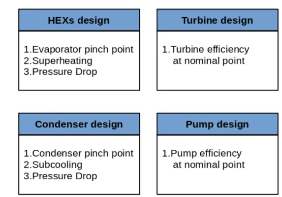
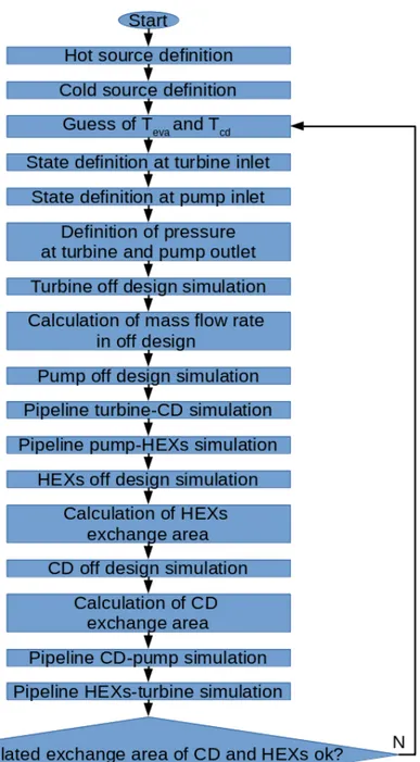
4.14 Input data for the design of the main components of the ORC at nominal conditions . 113 4.15 Algorithm of the ORC simulation model for off design . . . 115
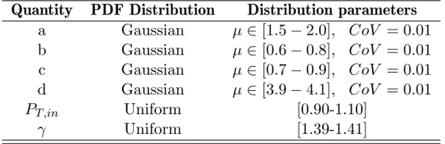
4.16 Input data for the simulation of the main components of the ORC in off design conditions116 4.17 RDO simplified scheme . . . 119
4.18 Histogram of the QoI WORC,net under uncertainty . . . 121
4.19 Total Sobol Index from Global sensitivity analysis . . . 121
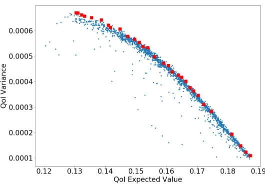
4.20 Objective space – CF1 vs CF2 . . . 123
4.21 Objective space – CF1 vs CF3 . . . 124
5.1 Baseline quasi-1D nozzle . . . 128
5.2 Assessment of UQ methods: approximate pdf of the QoI J for MC, BK and GEK. . . 133
5.3 Global sensitivity analysis with Sobol indexes . . . 134
5.4 Objective space . . . 135
5.5 Evolution of the convergence for BK, GEK, MoM and MF . . . 136
5.6 PDF of the QoI J for the optimal solutions in Tab.5.4 . . . . 138
5.7 Baseline geometry and optimized geometries (with 3σ uncertainty intervals) for various RDO strategies. . . 138
5.9 h-s chart with uncertainty at the inlet (blue hatched area) and at the outlet (red hatched
area) of the cascade . . . 143
5.10 Blade profile modelling with FFD . . . 144
5.11 Coarse mesh, with the identification of boundary surfaces . . . 146
5.12 Detail of the boundary layer over the blade surface in the medium mesh . . . 146
5.13 Detail of the trailing edge in the fine mesh . . . 147
5.14 Element mesh quality distribution for the medium grid . . . 147
5.15 Computational grid used for the validation of the CFD model . . . 151
5.16 Validation of the CFD model with test case [13] for air . . . 151
5.17 Validation of the CFD model with test case [14] for propane . . . 152
5.18 Entropy field in the baseline geometry . . . 153
5.19 Mach number distribution in the baseline geometry . . . 154
5.20 Pressure distribution in the baseline geometry . . . 155
5.21 Convergence to solution of QoI J vs. mesh refinement . . . . 156
5.22 Convergence to solution of Mout vs. mesh refinement . . . 156
5.23 Yplus in the simulation of the baseline geometry on the coarse mesh . . . 157
5.24 Yplus in the simulation of the baseline geometry on the medium mesh . . . 157
5.25 Yplus in the simulation of the baseline geometry on the fine mesh . . . 157
5.26 Objective space . . . 160
5.27 First generation in SMOGA convergence . . . 160
5.28 Generation after the first MOEI infill in SMOGA convergence . . . 161
5.29 Generation after the second MOEI infill in SMOGA convergence . . . 161
5.30 Generation after the third MOEI infill in SMOGA convergence . . . 162
5.31 Comparison of the baseline and the optimal solution found . . . 163
5.32 Comparison of the QoI PDF for the baseline geometry and the RDO optimum . . . . 163
5.34 Mach number distribution in the RDO optimal geometry . . . 165 5.35 Pressure distribution over the blade. Comparison between baseline and RDO optimum 165
6.1 Capacit´e ORC install´ee par an (adapt´e de [1]) . . . 174 6.2 Installation d’ORC par an [2] . . . 174 6.3 Exemple d’application employant un cycle non r´eg´en´eratif `a un niveau de pression [3] 175 6.4 Exemple d’une installation de 3,2 MW pour la r´ecup´eration de la chaleur r´esiduelle
d’une aci´erie [3] . . . 177 6.5 Classification de l’incertitude et des principales sources d’incertitude dans les solutions
informatis´ees [7] . . . 179 6.6 Esquisse g´en´erale du cadre des UQ [8] . . . 180 6.7 Repr´esentation sch´ematique du processus de conception d’un composant . . . 182 6.8 Flowchart of the BK-based SMOGA RDO process. . . 189 6.9 Tuy`ere de r´ef´erence quasi 1D . . . 193 6.10 ´Evaluation des m´ethodes UQ : pdf approximatif du QoI J pour MC, BK et GEK. . . 198 6.11 Analyse de sensibilit´e globale avec les indices de Sobol . . . 199 6.12 Objective space . . . 200 6.13 ´Evolution de la convergence pour BK, GEK, MoM et MF . . . 201 6.14 PDF de la QoI J pour les solutions optimales en Tab.5.4 . . . . 203 6.15 G´eom´etrie de base et g´eom´etries optimis´ees (avec des intervalles d’incertitude de 3σ)
pour diverses strat´egies de RDO. . . 203 6.16 Diagramme h-s avec incertitude `a l’entr´ee (zone hachur´ee bleue) et `a la sortie (zone
hachur´ee rouge) de l’aube . . . 204 6.17 Mod´elisation du profil des pales avec FFD . . . 206 6.18 Maillage grossier, avec identification des surfaces limites . . . 207 6.19 D´etail de la couche limite sur la surface de l’aube dans la maille moyenne . . . 208 6.20 D´etail du bord de fuite dans la maille fine . . . 209
6.21 R´epartition de la qualit´e des mailles des ´el´ements pour le maillage moyen . . . 209 6.22 Grille de calcul utilis´ee pour la validation du mod`ele CFD . . . 213 6.23 Validation du mod`ele CFD avec cas test [13] pour air . . . 213 6.24 Validation du mod`ele CFD avec cas test [14] pour propane . . . 214 6.25 Champ d’entropie dans la g´eom´etrie de base . . . 215 6.26 Distribution des nombres de Mach dans la g´eom´etrie de base . . . 216 6.27 Distribution de la pression dans la g´eom´etrie de base . . . 217 6.28 Convergence vers la solution du QoI J vs. raffinement du maillage . . . . 218 6.29 Convergence vers la solution de Mout vs. raffinement du maillage . . . 218
6.30 Yplus dans la simulation de la g´eom´etrie de base sur le maillage grossier . . . 219
6.31 Yplus dans la simulation de la g´eom´etrie de base sur le maillage moyen . . . 219
6.32 Yplus dans la simulation de la g´eom´etrie de base sur le maillage fine . . . 219
6.33 Objective space . . . 222 6.34 Premi`ere g´en´eration dans la convergence SMOGA . . . 222 6.35 G´en´eration apr`es le premier remplissage MOEI dans la convergence SMOGA . . . 223 6.36 G´en´eration apr`es le deuxi`eme remplissage du MOEI dans la convergence SMOGA . . 223 6.37 G´en´eration apr`es le troisi`eme remplissage du MOEI dans la convergence SMOGA . . . 224 6.38 Comparaison de la ligne de base et de la solution optimale trouv´ee . . . 225 6.39 Comparaison de la QoI PDF pour la g´eom´etrie de base et l’optimum RDO . . . 225 6.40 Champ d’entropie dans la g´eom´etrie optimale des RDO . . . 226 6.41 Distribution des nombres de Mach dans la g´eom´etrie optimale des RDO . . . 227 6.42 R´epartition de la pression sur l’aube. Comparaison entre la ligne de base et l’optimum
RDO . . . 228
Introduction
The Organic Rankine Cycle (ORC) is a viable technology for the exploitation of renewable energies like concentrated solar power, geothermal power, biomass or waste heat recovery. In these applications, it usually outperforms classic steam cycles for its simplicity, the lower operational costs and the higher thermodynamic efficiency [16].
ORCs are Rankine Cycles employing as working fluid complex organic compounds (hydrocarbons, silicon oils or refrigerants), instead of steam: they are closed cycles involving at least a pump, that compresses the working fluid, a group of hot heat exchangers, usually composed by one or more pre-heaters, an evaporator and sometimes also a superheater, where the working fluid is heated by an external heat source to become vapour; afterwards, there is a turbine, that converts the thermodynamic power of the fluid in mechanical one, and a condenser, where the residual heat is released at the environment allowing the fluid to come back to the liquid status. The mechanical power at the turbine shaft is converted in electricity by a generator.
During the last ten years, Organic Rankine Cycles (ORCs) have become a competitive technical solution for the exploitation of low-medium temperature heat sources of limited capacity [16], bringing about an extraordinary growth of their market, in particular for geothermal, biomass and waste heat recovery (WHR) applications. Data plotted in Fig. 1.1 and Fig. 1.2 show an explosion in the number of the ORCs installed since the early 2000s simultaneously combined with a rapid increase in the average size of these plants.
From Fig. 1.1 it arises that ORCs main field of application is geothermal power, even if this technology is characterized by a low number of installations: therefore, geothermal plants generally
geothermal fluid, brine and steam are separated: the first is employed to warm the liquid working fluid up in the pre-heater(s), while the second one is used to evaporate the organic working fluid. In any case, geothermal applications use generally saturated cycle configuration employing an alkane as a working fluid (the most common are pentane and butane). To enhance the heat recovery from geothermal brine, more pressure levels can be employed [18] and sometimes the system can include a regenerator to improve the cycle efficiency. An example of application employing a non regenerative one pressure-level cycle is depicted in Fig. 1.3.
Figure 1.3: Example of application employing a non regenerative one pressure-level cycle [3]
Biomass represents another quite widespread ORC application: starting from the early 2000, several high-temperature ORC power plants with the size of about 1 M We have been installed in
Europe to use various types of solid biomass [17]. Quite commonly, these plants are cogenerative, providing both electricity and heat, which is typically employed below 100 degC for district heating or for process purposes (e.g., wood drying). [19]. The majority of these systems adopts siloxanes like hexamethyldisiloxane or octamethyltrisiloxane as the working fluid in a superheated regenerative
needs [20].
Another application with an interesting potential for all unit sizes is waste heat recovery (WHR); in fact, many are the opportunities for heat recovery from the manufacturing and process industry [21]. According to data plotted in Fig.1.1 and Fig.1.2, this should be considered an emerging field for ORCs: on that market several solutions are available with medium and large size recovery solutions from gas turbines, internal combustion engines or industrial processes (i.e., cement factory, steel mill and glass factory). Usually in this application siloxanes, alkanes, cycloalcanes and some HFO refrigerant can be adopted in thermodynamic cycles that are generally superheated. Nowadays, this application is the one presenting the highest flexibility in the cycle configuration; a 3.2 MW plant for waste heat recovery from a steel mill is shown in Fig. 1.4.
Finally, solar applications are negligible if compared with geothermal power, biomass and WHR: this is probably due to the fact that ORCs could be coupled with concentrating solar power plants that for the moment are more expensive than photovoltaic panels and battery systems [1]. However, because of their high reliability, availability and performance, ORCs have been identified as the optimal conversion technology in this context [22, 23].
One of the biggest strength of ORC technology, that should be considered as one of the main reasons of their dramatic success, has probably to be found in their extreme flexibility, which allows them to be conveniently adapted to customer’s necessities; in fact, they are so much customizable that sometimes some tailor-made solutions proposed by the ORC suppliers can be considered as real engineering challenges in terms of design, construction, commissioning and operation. By moving from a project to another, a number of elements are likely to change; some of which are listed below.
1. The purpose of the application: pure electric power production or cogeneration of electric power and heat.
2. The type of heat source (geothermal or biomass or WHR or solar).
3. The ORC operating conditions, which may require different plant control solutions.
another usually can change dimensions and configurations.
5. The plant layout, depending on availability of room for all the components.
6. The working fluid.
7. The type of environment (indoor or outdoor) and the presence of acidity in case of geothermal plants.
8. Safety restrictions, depending on the country and the applications.
9. Regulations about fluids and their interactions with pollution (i.e. Montreal protocol or the European F-gas regulation).
mostly tailor-made plants since it is not possible to fully standardize ORCs. This is confirmed by inspection of commercial material (brochures, presentations or white papers) provided by the biggest ORC suppliers (for instance, see [24, 25, 26, 27, 28]).
Paradoxically, the large number of degrees of freedom left free when designing an ORC plant is at the same time a serious limitation. In fact, in order to better understand the dynamics of the ORC market, it is mandatory to identify the shareholders that usually buy ORCs to operate them: the large majority of the ORC plants that have been built until today and that are still in operation is property of privately held entities, which usually consider ORCs as an investment of a part of their resources to be analysed in terms of risk, payback time and return on investment; usually the revenues come almost exclusively from the amount of energy generated, which needs to be evaluated as accurately as possible.
Thus, despite the high level of confidence and know-how reached nowadays, usually a project concerning an ORC is still dominated by a large series of unknown variables which are related to the design, the commissioning, the operation and the decommissioning of the plant and which could reduce shareholders’ enthusiasm about ORCs. It is therefore mandatory to identify innovative techniques capable to deal with the uncertainty affecting ORCs: concerning the design of ORC components and whole ORC systems, robust design optimization (RDO) can be an answer to this issue.
In the following several RDO approaches are applied to ORC systems and to ORC turbo-expanders. The manuscript is organised as here described:
• Chapter 2 introduces the verification and validation framework for computer models of real systems and the definitions of uncertainty; afterwards, it presents the uncertainty quantification (UQ) methodology and it provides a quick outline of some techniques that are commonly used to propagate the uncertainty through the model and to quantify it.
• Chapter 3 depicts the deterministic design process of a system or of a component and it provides few elements about optimization. Afterwards, the robust design optimization is introduced and finally two RDO techniques specifically investigated in this work are introduced, namely the “two nested Bayesian Kriging” (TNBK) and the multi-fidelity (MF) approaches.
RDO based on Monte Carlo sampling: to perform this validation, a crudely simplified model of an ORC for WHR is employed. Once that this approach has been validated, it is used for the RDO of a real ORC system for geothermal application.
• Chapter 5 focuses on the application of both RDO techniques explained in Chapter 3 to the robust design optimization of turbo-expanders. First several UQ techniques are assessed for a toy test problem roughly representative of an ORC nozzle, i.e. a quasi 1D nozzle. Finally, the MF technique is applied to the RDO of a 2D cascade of stator blades for an ORC turbine. • Chapter 6 draws conclusions and provides some perspectives.
Uncertainty quantification
Contents
2.1 Verification and Validation . . . 32 2.2 Error and Uncertainty . . . 36 2.3 UQ Framework . . . 37 2.4 Overview about uncertainty propagation . . . 40 2.4.1 Monte Carlo method and improved sampling techniques . . . 40 2.4.2 Polynomial Chaos Expansion (PCE) . . . 43 2.4.3 Surrogate Models . . . 44 2.5 Uncertainty quantification methodology . . . 48 2.5.1 Methods of Moments (MoM) . . . 49 2.5.2 Bayesian Kriging (BK) . . . 49 2.5.3 Gradient Enhanced Kriging (GEK) . . . 57 2.6 Preliminary validations . . . 58 2.6.1 Simple analytic test functions . . . 59 2.6.2 UQ of a (simple) ORC . . . 68 2.7 Summary of the chapter . . . 74
The design of complex engineering systems increasingly relies on simulations based on computa-tional models predicting their behaviour. At a glance, these models can be considered as a black-box containing a mathematical description of the relevant phenomena. Since it is usually not possible to solve analytically the set of equations employed in it, a numerical solver is embedded in the model.
Considering that the model aims at reflecting the real world, once properly calibrated and validated with respect to experimental data, it becomes an important tool for decision-making. For instance, it can be used to explore the design space, i.e. to explore how the system response (model output) reacts to changes in the system input parameters, like geometry, operating conditions and model parameters.
Another possibility is to put an optimization loop upon the model, to find the best design according to some pre-defined criterion (cost functions). Finally, models can be employed for making predictions about future system behavior (forecasting).
The present Chapter first provides introductory concepts about model verification, validation and uncertainty quantification. A selection of methods for quantification and propagation of uncertainty of interest for the present study is also presented.
2.1
Verification and Validation
Using a model as a reflection of some real phenomena is a not-straightforward process and it should be done consciously. In fact, as depicted in Fig.2.1, it is mandatory to pass through two different types of models: a conceptual model and a computerized one.
Figure 2.1: Phases of modeling and simulation [4]
The first is constructed by analyzing and observing the physical phenomena of interest, since it aims to contain a more or less complete description of the system, based on governing equations and mathematical modeling from data [29]. In computational physics, the conceptual model contains the partial differential equations (PDE), or sometimes the ordinary differential equations (ODE), for conservation of mass, momentum, and energy; it also includes all auxiliary equations, such as
turbulence models, constitutive models for materials, and electromagnetic cross-section models, the initial conditions and the boundary conditions of the PDEs [5]. The step linking the reality with the conceptual model is referred to as model qualification and it requires the good knowledge of the real system.
To simulate the behaviour of the real system, the conceptual model is usually replaced by a nu-merical approximation; this provides a computerized model that is finally applied to solve engineering problems. Finally, the computerized model output is assessed against measurements of the real system (possibly affected by observation errors). Based on the results, the conceptual model may be improved, and so on.
The circular process just described includes several sources of error or uncertainty that must be taken into account, namely observational errors (which is object of metrology), modeling errors and discretization ones [6]. To control them, verification and validation have a central role in the assessment of the accuracy of the conceptual and computerized models; as a consequence, a huge bibliography exists about this topic and about methods and techniques related at them.
Figure 2.2: Verification process [5]
A thorough definition of verification has been provided by AIAA, as “the process of determining that a model implementation accurately represents the developer’s conceptual description of the model and the solution to the model” [30]. Thus, the emphasis in verification is pointed to the identification,
quantification, and reduction of errors in the numerical methods and algorithm used to solve the equations employed in the model, in order to provide evidence that the conceptual model is solved correctly by the discrete mathematics embodied in the computational code; to do this, verification is mainly based on benchmark and comparison with highly accurate solutions of test case that are available [29]. Fig. 2.2 shows that the verification test relies on demonstration: a comparison between the computational solution and the correct answer is carried out for the evaluation of error bounds, such as global or local error norms [5].
On the other side, validation has been defined as “the process of determining the degree to which a model is an accurate representation of the real world from the perspective of the intended uses of the model” [30]. Here, the main focus is on the process of understanding whether the right equations have been considered in the model for describing the real world. The fundamental strategy of validation involves identification and quantification of the error and uncertainty in the conceptual and computational models, quantification of the numerical error in the computational solution, estimation of the experimental uncertainty, and finally, comparison between the computational results and the experimental data, which are considered as the most faithful reflection of reality [5]. Fig.2.3 depicts the validation test, which is based on the comparison of the computational solution with experimental data.
As typical complex engineering systems are usually interested by multidisciplinary coupled physical phenomena occurring together, the validation test presents a remarkable amount of serious complica-tions: the quantities of interest (QoIs) are commonly not accessible for observation and, in any case, generally only just few experimental data, characterized by low quality and subject to uncertainty, are available. Consequently, because of the unfeasibility and impracticality of conducting true valida-tion experiments on the most of complex systems, it is usually recommended to use a building-block approach, which decomposes the system of interest into progressively simpler tiers [30, 31, 32, 33].
Once that all blocks the validation and verification (VV) approach for scientifically-based predic-tions have been here presented, the whole VV framework is represented in Fig.2.4. For further details about this topic, the reader is addressed to [6, 34].
Figure 2.3: Validation process [5]
2.2
Error and Uncertainty
Two key elements in the VV process just presented are the concepts of error and uncertainty, that are often used interchangeably in the colloquial language even if they differ significantly.
In a probabilistic framework, the error is “a recognizable deficiency in any phase or activity of modelling and simulation that is not due to lack of knowledge ” [30] so that its deterministic nature as a deficiency can be identified by means of examination [35]. In computerized solutions, there are five major sources of errors:
• discretization (spatial and temporal),
• insufficient convergence of an iterative procedure in the code solver,
• computer round-off,
• computer programming errors,
• improper use of the code.
As indicated in Fig.2.5, these can be classified in two sub-categories: acknowledged and unacknowl-edged errors. If the presence of the first one can be acceptable, as long as this kind of errors can be identified and quantified, for the second one instead, it is possible to identify them only by comparing the results with codes that set the benchmark; otherwise they cannot be found and removed from the code [7].
Unlike error, uncertainty is “a potential deficiency in any phase or activity of the modeling process that is due to the lack of knowledge” [30], revealing a clear stochastic nature [35] as long as the lack of knowledge can occur in the physical models or in the input parameters, with a potential risk to affect the reliability of the simulation.
Uncertainty can be classified in two categories: the aleatory and the epistemic uncertainty. The first one is connected to the physical variability within the system or its environment and it cannot be reduced: the only way to treat it is just to characterize it by performing additional experiments, in order to get more data modelling the variables that can be used consequently in a probabilistic approach. On the other side, the epistemic uncertainty arises from the assumptions and from the simplifications made in deriving the physical formulation: thus, it can be considered reducible by performing more experiments and using the information to improve the physical models.
As depicted in Fig.2.6, several sources of uncertainty exist for a computerized model. With re-gards to aleatory uncertainty, these are the randomness of the system parameters (geometric variables, material properties, manufacturing tolerances) and the randomness of the environment (initial and boundary conditions and environmental parameters). Epistemic uncertainty is largely related to un-certainties in model selection, which typically stems from a lack of knowledge about the underlying physics or from the impossibility to use a complete and accurate model to simulate them [36].
2.3
UQ Framework
Probabilistic engineering aims to take into account the uncertainties appearing in the modeling of physical systems and to study the impact of those uncertainties onto the system response [37]. To this end, a well established and universally accepted framework for the quantification of the uncertainty has been developed: it is a circular multi-step process whose guidelines are presented in Fig.2.7 and hereafter briefly described.
Figure 2.6: Classification of uncertainty and major sources of uncertainty in computerized solutions [7]
Step A consists in defining the model that should be used to reflect the physical system under consideration as already described in Section 2.1: this stage gathers all the ingredients used for a classical deterministic analysis of the physical system to be analyzed. Moreover this is the step where the QoIs are selected.
Step B corresponds to the quantification of the sources of uncertainty, by identifying the input pa-rameters that cannot be considered as well-known because they are affected by uncertainty; therefore, they are modelled in a probabilistic context, through the definition of their PDFs. Typically, stochas-tic inputs can be associated with the operating conditions [38, 39, 40], the geometry [41, 42, 43, 44] as well as the empirical parameters involved in the physical models, e.g. in turbulence models [45] or the equation of state (EoS) [46]. The final product of this step is a vector of random variables having a well established probability distribution function (PDF).
Step C is the most computationally demanding one of the process, as it consists in propagating through the model all the uncertainties in the inputs, characterizing the random response appropriately with respect to the assessment criteria defined in Step A: usually, the objective of this phase is the computation of the probability distribution function of the QoI or of its statistical moments. Monte Carlo (MC) sampling is probably the most intuitive method to carry out this task, but it requires also a lot of computational resources, because it gives an entire discrete probability distribution (histogram) of the QoI as an output. In order to reduce the computational effort, some other methods are commonly used as they are faster than MC; some of them are described in the next section.
Once that the uncertainty has been propagated through the model, it is possible to perform a sensitivity analysis to get some information about the respective impact of the random input variables on the QoIs; in fact, the more complex the system is, the larger the number of input parameters becomes, and the designer will be probably interested in understanding the effects of each of them on system response. Thus, once that the PDFs (or just the statistics) of the QoIs have been computed, they can be used to characterize the output, in order to improve the knowledge about the considered problem.
Generally, two main approaches exist for sensitivity analysis, i.e. the local and the global. The first one is probably the most intuitive method as it analyses the impact on the QoI of small perturbation of the uncertain variables around their nominal values: this is done calculating the partial derivatives of the QoI with respect to the uncertain variables. Usually these quantities are derived by means of the
One-At-Time (OAT) method (the interested reader can find thorough review of this basic technique in [47]). However, the local approach presents several limitations, such as the assumptions of linearity and normality and it suffers in case of dependency among the uncertain variables [48]. On the other hand, the global sensitivity approach is based on the analysis of variance (ANOVA) decomposition [49], and then it estimates Sobol indexes [50] associated to the uncertain inputs. In the following, this last approach is the only one used to perform sensitivity analysis. The interested reader is referred to Appendix B for more details about it.
2.4
Overview about uncertainty propagation
Various techniques for uncertainty propagation are briefly reviewed hereafter; first the focus is put on Monte Carlo and some improved sampling methodologies and then the polynomial chaos expansion techniques and some surrogate-model based approaches are presented.
2.4.1 Monte Carlo method and improved sampling techniques
Developed at the begin of 40s of the last century within the Manhattan project [51, 52], the MC method consists of random sampling of the input variables according to their own distributions and propagation of the resulting values through the model, which is run in deterministic mode for each sample. The output of the sampling process is an entire distribution of the QoI that can be analyzed with tools from statistics [51, 53].
As described in Fig.2.8, Monte Carlo approach consists in drawing samples from the input PDFs, and to compute for each of them the corresponding model outputs for the QoIs. The results may be used to construct an histogram of the output QoIs or to compute means and variances. The MC method has several advantages: it is well-posed, it has good convergence properties and, since it is non-intrusive, it does not need to have access to the equations employed in the model. Unfortunately, a very large number of samples is required to converge the statistics, which makes the Monte Carlo approach inapplicable to costly models: thousands or even millions of samples (each of them involving a model run) are required in order to get a good estimation of the QoI with enough accuracy. Precisely, the MC method shows convergence to the exact stochastic solution of √1
N, where N is the number of
Figure 2.8: Monte Carlo process
Both LHS and LBS methods can be considered as improved sampling techniques, because they have been developed for reducing the number of model runs of the MC, aiming to get equally accurate results with a significant decrease in computational time.
LHS [55] is one of the most widely used alternative to the standard random sampling of MC method. In fact, assuming to have a d-dimensional vector ξ of uncertain input parameters, it has been just shown that MC method randomly samples N vectors ξi as represented in Eq.2.1.
ξi = (ξi1, ξi2, ..., ξid) f or i = 1, 2, ..., N (2.1)
In LHS, the range of probable values for each uncertain input parameter of ξ is divided into N non-overlapping segments of equal probability. Subsequently, for each uncertain input parameter of ξ, one value is randomly selected from each interval, by following the probability distribution on the interval. In this way it is possible to obtain d sequences of N numbers and to built the ξi vectors by pairing randomly the entries in these sequences. Obviously in order to work properly, LHS must have a memory, while this is not true for MC method. To better understand this technique an example is presented in Fig.2.9: for a set of size N = 5 and two input random variables ξ = (ξ1, ξ2) , where ξ1
Figure 2.9: LHS, size N = 5 and two random variables
is a Gaussian distribution (Fig.2.9 a) and ξ2 is a uniform distribution (Fig.2.9 b). A possible LHS for
this case is shown in Fig.2.9 c.
A more detailed description of LHS technique is available in [56], where it is shown also that, since the occurrence of low probability is reduced, the convergence is faster than standard MC, providing however an optimal convergence of the parameter space.
As indicated by the name, LBS is based on lattices, which can be seen as discrete repeating arrangements of points in a grid pattern. Thus, for each variable the entire range of probable values is again divided, but in this case the discretization is made using regularly spaced points and the solutions are evaluated at those points The characteristics of the lattice are strictly related to the distribution of the input variables [57]. An example of a lattice based sampling for a two-variable problem is shown in Fig.2.10. Usually LBS is used for for simulations dealing with condensed matter
Figure 2.10: Lattice based sampling technique for a two variable problem
physics or nuclear physics [7].
Several more improved sampling techniques exist (i.e. Low Discrepancies Sequences [58, 59]), but a detailed description of them is out of the scope of the present work; the interested reader can refer to [57, 60]. However, even if they are faster than the standard MC, they remain too much expensive for complex models and large parameter spaces. For this reason, in order to reduce computational resources, they can be used with surrogates models, as it is discussed in the next section.
2.4.2 Polynomial Chaos Expansion (PCE)
A large class of methods for uncertainty propagation is based on the polynomial chaos framework [61]: both intrusive and non-intrusive variants exist [62]. The implementation of intrusive uncertainty propagation methods requires access to the source code of the model; this formulation has two main drawbacks: first, the availability of the source code of the solver and, second, the need to modify the code as soon as the nature or number of uncertain parameters changes, the polynomial chaos order is modified, or different modeling choices are introduced. On the other hand, non-intrusive methods use the deterministic solver as a black-box for uncertainty propagation: this allows the application
of uncertainty propagation methods in combination with commercial or in-house solver. However, the number of samples required by PCE is greatly reduced in comparison with a full Monte Carlo simulation to get the same accuracy. As both the intrusive and the non-intrusive approaches are based on polynomial chaos expansion, the PCE framework is here quickly presented.
A polynomial chaos is a polynomial of random variables instead of ordinary variables [62]; it is based on the homogeneous chaos theory of Wiener [63], who constructed a chaos expansion using Her-mite polynomials. Ghanem and Spanos [61] provided the basis for the current spectral stochastic finite element methods, like the Generalized Polynomial Chaos method (gPC) [64] and the Gram-Schmidt Polynomial Chaos method [65]. Since a Galerkin projection is used to obtain the polynomial chaos coefficients, these methods are referred to as Galerkin Polynomial Chaos methods: they are proba-bly the most intuitive PCE approach, but they have also a relatively cumbersome implementation, primarily due to the fact that it requires the availability of the solver source code; furthermore the equations for the expansion coefficients are almost always coupled [66]. In case of high complexity in the original problem, the explicit derivation of the gPC equations can be impossible.
Thus, non-intrusive implementations of PCE are generally employed: usually they rely on two different approaches, namely the pseudo-spectral form [67, 68] and the stochastic collocation method [69, 70, 62, 38, 71]. However, they both face the drawback that computational cost for the estimation of the statistics increases exponentially with the number of uncertain variables: this problem, known in UQ as curse of dimensionality [72, 73]), limits the applicability of the method to spaces not larger than 4 or 5 dimensions. A possible solution to alleviate curse of dimensionality consists in using sparse grid methods [74, 75, 76], simplex stochastic collocation method [77, 78] or Smolyak-based sparse pseudospectral approximations [79, 80, 81].
Another way to reduce curse of dimensionality consist in using adaptive techniques: a classic approach can be found in [82, 83, 84]. More advanced implementations exists; the interested reader can refer to [85, 86, 87, 88]
2.4.3 Surrogate Models
The basic idea in the surrogate model approach is substantially to build a fast mathematical approximation of the real model, which is too expensive in terms of computational resources. Thus, “given these approximations, many questions can be posed and answered, many graphs can be made,
Figure 2.11: General use of surrogates for problem analysis or optimization
many trade-offs explored, and many insights gained. One can then return to the long-running computer code to test the ideas so generated and, if necessary, update the approximations and iterate” [89]. The term “surrogate model” is often used interchangeably with the terms “metamodel” or “response surface model”.
There are several types of surrogate model and each one needs to be built with its proper technique, but generally the way to employ them is very similar, as shown in Fig.2.11. The process always starts with the construction of a sampling plan, also called design of experiment (DOE): the domain space of the input parameters is covered with several points that are selected according to the distribution of each input parameter. For instance if a parameter of the problem has a uniform distribution, it will
be subject to a uniform sampling. Typically, in this part of the process, random sampling, LHS, LBS or another improved sampling techniques are used.
Afterwards, since all these techniques rely on the data coming from the DOE, the original model is run for all the selected points, as in a MC simulation: the only difference lies on the fact that a MC simulation needs a huge amount of points in order to build an output distribution, while the DOE samples are required just to train and to test the surrogate model.
Once that the cheaper surrogate model has been built, it can be used to perform visualization activities, (i.e. the exploration if the design space, sensitivity analyses or uncertainty quantification) or optimization, (i.e. the adjustment of system parameters to maximize/minimize one or more cost functions). Independently from the application, as the surrogate is only an approximation of the full model output estimates of some techniques for evaluating the approximation error are required. Surface response enrichment by inclusion of additional observation(s) can be used to improve the surrogate quality.
Using a surrogate allows considerable gains in computational effort: for instance, in UQ applications there is usually a difference of 2-3 orders of magnitude in computational time between surrogate-based sampling and the brute MC method to get the same accuracy in the approximation of the PDF of the QoI [90].
Moreover, many surrogate models are non-intrusive, since it is not necessary to have access to the equations of the original model, which can be run in black-box mode for all the points in the DOE. Finally, the surrogate model approach can also benefit of parallelization; in fact, every run is independent from the other and consequently it can be solved in parallel on a High Performance Computing Infrastructure.
With regards to quantification of uncertainty, surrogates can be divided in two main category. The first group is composed by deterministic methods: they first determine the sensitivities of the uncertain parameters, and then they combine this information with the covariance matrix of the input parameters, to obtain an estimation of the statistical moments of the QoI PDF [91]. The second category contains stochastic-based techniques, which relies on probabilistic approach since they first require that the uncertainty of the input parameters is characterized by a PDF (e.g. normal, beta, lognormal,etc.); afterwards random samples are generated from the PDFs of the uncertain parameters
and these samples are propagated through the numerical model [92]. These methods allow to construct an approximation of the QoI PDF or they can be simply employed to calculate its statistical moments. An example of deterministic method is the so-called first-order Method of Moments (MoM) [93], which approximate statistical moments of the QoI by Taylor series expansions. Such method can be remarkably fast if derivatives of the cost function with respect to the uncertain variables are readily available by means of a discrete or continuous adjoint solver [94, 95, 96, 97, 98, 99]. Nevertheless, its accuracy is limited to Gaussian or weakly non-Gaussian processes with small uncertainties, since higher-order terms become increasingly important for strongly non-Gaussian input distributions. Some improvement can be achieved by using higher-order expansions, but these require information about higher-order sensitivity derivatives, which may represent a delicate and highly intrusive task. A more complete discussion can be found in [100].
On the other hand, a stochastic UQ method is the radial basis functions approach: in engineering it is usual practice to use a polynomial approximation. Polynomials are generally restricted to low order approximations, especially in high dimensional problems [89]. Increased flexibility in the approx-imation can be achieved by adding further approxapprox-imations to the polynomial surface with each one centered around one of the n sample points, as discussed in [101] or in [102] . This approach is known as radial basis functions. However, in case of complex or parametric basis functions, the additional task of estimating any other supplementary parameters should be considered; a typical example of a situation like this is the estimation of σ term in the Gaussian basis function, that as a result is usually taken to be the same for all basis functions [89]. Thus, for high-dimensional problems with a large number of sample points this approach turns out to be unwieldy.
Another stochastic method for the UQ is Kriging, which has emerged just in the last years as a powerful tool for building meta-models, even if it has been used (with different names) by Wiener [103, 104] and Kolmogorov [105, 106]. Historically Kriging opened the field of geostatistics, formalized by Matheron [107, 108] and it was named like this in order to honor the seminal work of the South African engineer D. Krige, who initiated a statistical method for evaluating the mineral resources and reserves [109]. A detailed dissertation about the theory which is behind this technique and about its employment in geostatistics is provided also in Cressie [110] and in Stein [111]. Sacks et al. [112] introduced the key idea that Kriging may also be used in the analysis of computer experiments in which:
• the data is not measured but results from evaluating a computer code, i.e. a simulator such as a CFD code or a finite element code;
• the points where data is collected are not physical coordinates in a 2D or 3D space, but param-eters in an abstract space of arbitrary size.
Nowadays Kriging is considerably studied and applied as a prediction tool in economics and in machine learning, fields in which it is known as Gaussian Process (GP) technique.
In contrast to polynomial chaos expansions, Kriging provides a meta-model that does not depend on the probabilistic model for the input random vector [90]. In fact, The basic idea of Kriging is to model some function known only at a finite number of sampling points as the realization of a Gaussian Process (GP), which is defined as a collection of random variables, any finite number of which have a joint Gaussian distribution and it is completely specified by its mean and covariance functions [113].
2.5
Uncertainty quantification methodology
One should consider a set of QoIs J :
J = J (x, ξ) (2.2)
with J ∈ Rm depending on a vector of deterministic design parameters x ∈ Rndes and on a vector
of uncertain parameters ξ ∈ Rnunc. One should note that some of the design parameters may also
be uncertain. The objective of the UQ problem is the accurate estimation of the expectancy and the variance of the PDF of the QoI J , namely E[J ] and var[J ], given variations in the uncertain parameters; this methodology is based on a set of N deterministic samples of the solution J∗. For sake of simplicity, in the following, only the case of a single QoI (m = 1) is considered, but the approach can be extended to multiple QoIs. Moreover, since the design parameters are considered to be uncertainty-free, the dependency of J on x is for the moment neglected. The required statistics of the PDF of the QoI J are calculated by means of the deterministic MoM and the stochastic Kriging, implemented in a Bayesian framework; furthermore, the formulation of the gradient enhanced Kriging (GEK) is provided.
2.5.1 Methods of Moments (MoM)
Among deterministic UQ methodologies, an interesting approach is the MoM, which approximates the statistical moments of the fitness function by Taylor series expansions. This method may provide fast and sufficiently accurate estimates of the QoI statistics, as long as the fitness sensitivity derivatives with respect to uncertain parameters are provided by an efficient method and complete output statistics are not required [93]. Both first- and second-order MoM formulations have been considered in the literature (see for instance [96]). Here, the focus is restricted on the first-order MoM. Following [35], the first-order approximation for the expected value (mean) of J is simply given by:
E [J (ξ)] = J (ξ¯) (2.3)
which is nothing but the deterministic evaluation of function J at the mean value of the input ξ¯. The first-order variance is:
var [J (ξ)] = N ∑︂ i=1 N ∑︂ j=1 ∂J ∂ξi ⃓ ⃓ ⃓ ⃓ ξ ¯ ∂J ∂ξj ⃓ ⃓ ⃓ ⃓ ξ ¯ cov(ξi, ξj) (2.4)
with cov(ξi, ξj) the covariance matrix. If the variables ξ = {ξ1, ξ2, ....ξN} are uncorrelated, the covariance
is a diagonal matrix and Equation (2.4) takes the simplified form:
var [J (ξ)] = N ∑︂ i=1 N ∑︂ j=1 ∂J ∂ξi ⃓ ⃓ ⃓ ⃓ ξ ¯ ∂J ∂ξj ⃓ ⃓ ⃓ ⃓ ξ ¯ σi2 (2.5)
where σi2 stands for the variance of the i-th uncertain parameter.
2.5.2 Bayesian Kriging (BK)
In general, the unknown QoI J , depending on a set of uncertain variables ξ with dimension
nunc= M , is modelled as a regression function of the form:
J(ξ) = m(ξ) + Z(ξ) (2.6)
where:
1. m(ξ) =∑︁
ifi(ξ)βi is the mean of the process.
3. βi are the regression coefficients to be calculated for the mean of the process.
4. Z(ξ) = GP (0, P) is a stationary zero mean Gaussian process with covariance function P, mod-eling the deviation between the regression function and the data, that needs to be evaluated.
This Kriging formulation can be revised in the Bayesian framework (see for instance [114, 115, 116, 117]), which is particularly suitable to deal with the uncertainty of the model parameters and to provide a compensation in case of availability of only few measurements [118, 119]. Therefore, considering N sampling points contained in the design of experiment (DoE) ξ∗, which is a matrix with dimension N × M , and the vector of the observed data J∗ = J (ξ∗), with dimension N composed by the evaluation of the QoI in the N samples ξ∗, this approach is founded on Bayes’ theorem, that is one of the cornerstones of Bayesian inference and it is summarized by Eq. 2.7:
p(J|J∗) = p(J ∗|J)p(J) p(J∗|ξ) (2.7) where: • p(J|J∗) is the posterior, • p(J∗|J) is the likelihood, • p(J) is the prior, • p(J∗|ξ) is the evidence.
The observed data vector J∗ should be thought as a subset of the QoI J selected by means of the observation matrix H, whose formulation is given in Eq. 2.8.
Hij =
{︄
1, if i = j
0, otherwise i = 1, ..., M and j = 1, ..., N (2.8) The likelihood in Eq. 2.7 comes from the sampling distribution as it is the conditional probability to observe the N data J∗ given the unknowns J and, because of the assumption that it is Gaussian distributed, it is formulated as in Eq. 2.9:
where R is the covariance of the observation error, that in the present work is considered uniform and uncorrelated, so that R = σ2I, with I equal to the identity matrix and σ which is a predefined error of the observed variable values.
The prior in Eq. 2.7 expresses the prior knowledge over the vector of the unknown QoI J (ξ) and, as it is also assumed to follow a Gaussian distribution, it is considered p(J ) ∼ N (0, P); moreover, the evidence in Eq. 2.7 is also Gaussian, as it is the marginalization of the likelihood over the prior [113]. As the right hand side of Eq. 2.7 is Gaussian, the posterior distribution obtained by means of the Bayesian framework just presented is calculated as a Gaussian distribution whose formulation is expressed in Eq. 2.10 [115].
p(J|J∗) ∼ N (E [J|J∗] , var [J|J∗]) (2.10)
where:
1. the mean E [J|J∗] = PHT(︂R + HPHT)︂−1J∗
2. the variance var [J|J∗] =
[︃
I − PHT (︂R + HPHT)︂−1
]︃
P
Finally, once that the posterior is available, it can be used to predict the values J′ = J (ξ′) of the QoI on the prediction points ξ′: as expressed in Eq.2.11, the predictive distribution J (ξ′) can be obtained averaging the output of all possible linear models with respect to the posterior distribution [113].
p(J′|ξ′, J) = ∫︂
p(J′|J, ξ′)p(J|J∗)dJ (2.11)
Generally, for the most of the models, the integral in Eq.2.11 is not easily tractable, but Kriging can be considered as an exception to this statement, because of the properties of Gaussian distribution. In fact, the predictive distribution is again a Gaussian, with the predictive mean equal to the posterior mean and the predictive covariance equal to the sum of the posterior covariance and the covariance of the observation error R (Eq. 2.12).
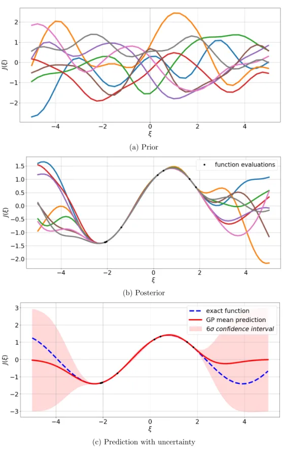
(a) Prior
(b) Posterior
(c) Prediction with uncertainty
For a better understanding of the technique just described, the whole process of the Kriging method in Bayesian framework is depicted in Fig.2.12. At the beginning there are no function evaluations available, and the prior is supposed to be an infinite collection of random pathlines; to fix ideas, in Fig.2.12a just eight of these pathlines have been depicted. The evaluation of the function J (ξ) in some points allows to improve the knowledge about J and to compute the posterior by means of Eq. 2.10; in Fig.2.12b only eight posterior realization are shown. Finally, once that the information about the posterior is available, it can be used to perform the prediction considering also the uncertainty about the model; in Fig.2.12c this uncertainty is represented by a 6σ confidence interval.
To complete the description of the BK method, some information about the covariance function P must be provided. This must be semidefinite positive and it is sometimes also referred to as Kernel. The most widely-used kernel within the kernel machines field is probably the squared exponential (SE), whose formulation is provided in Eq.2.13.
covSE(ξi, ξj, θ) = exp (︃ −(ξi− ξj) 2 2θ2 )︃ (2.13) where:
• ξ is the generic coordinate of the prediction y.
• ξi− ξj is the correlation range.
• θ is a parameter defining the characteristic length-scale (positive).
θ is a hyperparameter, that needs to be estimated using the data available from the prior
distribu-tion. The shape of the SE kernel as a function of hyperparameter θ is represented in Fig.2.13a, while Fig.2.13b depicts an example of prior sample paths generated by this covariance function.
The SE covariance function is infinitely differentiable, which means that the GP with this covariance function has mean square derivatives of all orders, and is thus very smooth [113]. Stein [111] argues that such strong smoothness assumptions are unrealistic for modeling many physical processes, and he recommends therefore the Mat´ern class of covariance functions (Eq.2.14).
covM atern(ξi, ξj, l, ν) = 21−ν Γ(ν) (︃√2ν(ξ i− ξj) l )︃ν Kν (︃√2ν(ξ i− ξj) l )︃ (2.14)
(a) Dependence from the θ hyperparameter.
(b) Example of prior pathlines (θ = 1).
where:
• ν and l are 2 hyperparameters (both positive).
• Γ is the Gamma function.
• Kν is the modified Bessel function of the second kind.
Figure 2.14: Dependence of the Mat´ern class of covariance functions from the ν hyperparameter
The dependence of the Mat´ern class of covariance functions from the ν hyperparameter is depicted in Fig.2.14. Usually the most common cases are ν = 3/2 and ν = 5/2, while for ν = 1/2 the process becomes very rough and ν ≥ 7/2 is usually avoided because it is commonly difficult to distinguish be-tween the values from finite noisy training examples, unless there is the explicit prior knowledge about the existence of higher order derivatives. For ν −→ ∞, the Mat´ern Covariance function becomes the smooth Squared Exponential one. l can be considered as a hyperparameter defining the characteristic length-scale (like θ in the Squared Exponential covariance function). Assuming ν = 5/2 , the shape of the Mat´ern kernel as a function of l hyperparamater is represented in Fig.2.15a, while Fig.2.15b depicts an example of prior sample paths generated by this covariance function.
A multitude of other possible families of covariance functions exists. The interested reader can find more information about this topic in [113]. To estimate hyperparameters, the Maximum Likelihood
(a) Dependence from the l hyperparameter (ν = 5/2).
(b) Example of prior pathlines (l = 1, ν = 5/2).
![Figure 2.6: Classification of uncertainty and major sources of uncertainty in computerized solutions [7]](https://thumb-eu.123doks.com/thumbv2/123doknet/2842221.69577/39.892.171.717.183.574/figure-classification-uncertainty-major-sources-uncertainty-computerized-solutions.webp)