Numerical investigation and experimental validation of a plasticity model for sheet steel forming

Technology researchers and makes it freely available over the web where possible.

This is an author-deposited version published in: https://sam.ensam.eu Handle ID: .http://hdl.handle.net/10985/9909

To cite this version :

Tales CARVALHO RESENDE, Tudor BALAN, Salima BOUVIER, Farid ABED-MERAIM, Simon-Serge SABLIN - Numerical investigation and experimental validation of a plasticity model for sheet steel forming - Modelling and Simulation in Materials Science and Engineering - Vol. 21, n°1, p.28p. - 2013

Numerical investigation and experimental validation of a

plasticity model for sheet steel forming

Tales Carvalho-Resende1,2,3, Tudor Balan1*, Salima Bouvier2, Farid Abed-Meraim1, Simon-Serge Sablin3

1 _{Laboratoire d'Étude des Microstructures et de Mécanique des Matériaux,} LEM3, UMR CNRS 7239, Arts et Métiers ParisTech, 4 rue Augustin Fresnel, 57078 Metz Cedex 03, France

2 _{Laboratoire Roberval de Mécanique, UMR CNRS 6253, Université de}

Technologie Compiègne, Centre de Recherches de Royallieu, BP 20529, 60205 Compiègne cedex, France

3 _{Technocentre Renault – Vehicle Engineering – Materials Engineering} Department – 1 avenue du Golf, 78288 Guyancourt cedex, France * Corresponding author: tudor.balan@ensam.eu, tel +33.3.87.37.54.60, fax +33.3.87.37.54.70

Abstract. This paper investigates a recently developed elasto-plastic constitutive model. For this purpose, the model was implemented in a commercial finite element code and was used to simulate the cross-die deep drawing test. Deep drawing experiments and numerical simulations were conducted for five interstitial-free steels and seven dual-phase steels, each of them having a different thickness and strength. The main interest of the adopted model is a very efficient parameter identification procedure, due to the physical background of the model and the physical significance of some of its parameters and state variables. Indeed, the dislocation density, grain size, and martensite volume fraction explicitly enter the model’s formulation, although the overall approach is macroscopic. For the dual-phase steels, only the chemical composition and the average grain sizes were measured for the martensite and ferrite grains, as well as the martensite volume fraction. The mild steels required three additional tensile tests along three directions, in order to describe the plastic anisotropy. Information concerning the transient mechanical behavior after strain-path changes (reverse and orthogonal) was not collected for each material, but for only one material of each family of steels (IF, DP), based on previous works available in the literature. This minimalistic experimental base was used to feed the numerical simulations for the twelve materials that were confronted to deep drawing experiments in terms of thickness distributions. The results suggested that the accuracy of the numerical simulations is very satisfactory in spite of the scarce experimental input data. Additional investigations indicated that the modeling of the transient behavior due to strain-path changes may have a significant impact on the simulation results, and that the adopted approach provides a simple and efficient alternative in this regard.

KEYWORDS: Metal forming; Interstitial Free steels; Dual Phase steels; Elasto-plastic model; Non-linear strain paths; Cross-Die test; Finite Element Method.

1. Introduction

Environmental, economic and safety concerns are driving car manufacturers to produce lighter and safer vehicles. In recent years, dual phase (DP) and other high strength steels are increasingly used for sheet metal parts in the automotive industry to meet these demands. Due to the lack of knowhow in forming these new materials and the short development times in the automotive industry, the numerical simulation has become a common tool for the sheet forming process development and optimization. The constitutive model and its material parameters are recognized as a primary factor in achieving the accuracy of the predictions of such finite element simulations, especially in terms of formability and springback. As a consequence, research efforts are continuously devoted to increasing the physical contents of the plasticity models – i.e. to relate more closely the internal variables and parameters of the models to metallurgical data. On the one hand, the resulting models can be used in the metallurgical industry to design new materials (i.e. microstructure, chemical composition, texture, etc.) in order to achieve some targeted final properties. On the other hand, these models involve fewer arbitrary material parameters that require specific mechanical tests to be determined, thus reducing the cost of the parameter identification for the application e.g. in the automotive industry. This was the main motivation for the work reported in this paper. Several categories of physically-based plasticity models have been developed in the past decades. Very rich metallurgical information could be imbedded in one-dimensional models describing the dislocation density motion and interaction at intra-granular scale (see, e.g., [1-3]). The yield stress evolution during monotonic loading can be related to the total dislocation density with the so-called Taylor relation

0 M Gb

σ

=

σ

+

α

ρ

, (1)

where

σ

₀ is the stress related to lattice friction and solute contents, G is the shear modulus, b is the magnitude of the Burgers vector, α is a factor that weights the dislocation interactions, and the transition from the grain scale to the macroscopic scale involves the so-called average Taylor factor M for the polycrystal. In the case of strain reversal, the tension-compression stress differential (back-stress) X related to the so-called Bauschinger effect has also been expressed recently by Sinclair et al. [4] as

Gb

X = M n

D , (2)

where D is the grain size and

n

is related to the number of dislocations that are stopped at the grain boundary on a given slip system; it saturates rapidly at a constant value n0. Although restricted to particular loading modes, these scalar models do not involve arbitrary parameters and they provide a first approximation of the material’s response without any prior

experimental test, using solely the chemical composition and microstructural data as input. In polycrystalline metals, the crystallographic texture is a source of plastic anisotropy, which can further evolve during plastic deformation. This feature can be described by models combining crystal plasticity and homogenization techniques. Taylor’s simple homogenization scheme [1] was the basis for more refined models [5]; alternative approaches were based on the self-consistent method [6-8], the crystal plasticity finite element method [9], etc. Such constitutive models can be applied at each integration point of a finite element model [10]. However, this requires huge calculation resources for metal forming applications. Proposed

approaches to reduce this numerical effort include, e.g., the use of an artificial scattering of the crystal orientations from integration point to integration point [11] or the modeling of an isotropic background of the texture plus a small and fixed number of texture components of variable weight [12, 13]. Full micromechanical models may be used to calculate only a small part of the yield locus, in the vicinity of the current loading point [14, 15]. Alternatively, the entire yield surface can be approximated by plastic potentials whose parameters are fitted with respect to a Taylor-model approximation of the initial anisotropy [16-18]. The parameters of such potentials can be further updated to account for the evolution of the anisotropy. This evolution is predicted by a micromechanical model for a reduced number of loading paths, inspired from the current process simulation, by means of a two-scale parameter identification technique. Various combinations of micromechanical models, macroscopic potentials and identification / interpolation techniques were proposed, e.g., in [19-21]. This is still an active field of research; in the current work the evolution of the plastic anisotropy is neglected and the initial anisotropy is simply approximated by a macroscopic yield surface. For the

application to mild and dual phase steels, Hill’s quadratic yield surface was adopted. Classically, hardening is also described in finite element codes with phenomenological functions of the plastic strain, whose parameters are identified to fit a set of mechanical tests performed on samples of the given material. In the last decades, advanced hardening models have been designed in a fully three-dimensional framework to describe the complex transient behavior of sheet metals after strain-path change, by modeling the most salient features of the dislocation structure evolutions in an average sense [22-24]. The increasing complexity of these models is compensated by an improved accuracy of process simulation [25, 26]; on the other hand, the cost of the parameter identification increased dramatically and became the primary obstacle for the application of these models in an industrial environment.

The current study contributes to the research efforts aiming to promote constitutive models that blend the physical insight of metallurgical models with the generality and efficiency of full three-dimensional macroscopic models, in an attempt to reduce the cost of parameter identification. Such models use scalar dislocation densities as internal variables, along with many of the associated physical parameters. A reduced set of fitting parameters is required to account for the scale transition from the grain to the polycrystal. Associated with the other metallurgical parameters, these fitting parameters are claimed to be characteristic of a whole family of materials, thus reducing even more the required identification effort. The aim of the paper is to investigate the ability of the constitutive model proposed by Carvalho-Resende et al. [27] to accurately predict sheet metal forming processes for a variety of mild and dual phase sheet steels, in the context of a reduced parameter identification procedure. The model’s equations are summarized in Section 2. The investigated materials are presented in Section 3, as well as the cross-die deep drawing test selected for the analysis. The simulation results are presented in Section 4 and compared to the experimental deep drawing results in terms of thickness distribution.

2. Constitutive model

In metal forming, the sheet generally undergoes large deformations, and its behavior is described by rate constitutive equations. We follow here a classical approach of

rate-independent macroscopic elasto-plasticity, defined by four ingredients: a hypo-elasticity law, a yield function, a (normality) flow rule and a set of hardening equations. This framework is

well documented in the literature (see, e.g., [28]); only its main equations are recalled here for completeness. The material is assumed orthotropic, which is commonly the case for rolled sheet metals. A stronger approximation is further adopted by considering that the material remains orthotropic during the deformation. The evolution (i.e., rotation) of the material symmetry frame is not mentioned here as it is regularly handled by the finite element code itself (see, e.g., [29]). The components of the stress and other tensorial state variables that enter the equations hereafter are expressed in this particular frame. This commonly adopted strategy allows for a simple constitutive formulation respecting the principle of material frame-indifference [28, 30, 31]. The material is initially stress-free (a well-annealed state) and homogeneous.

The Cauchy stress rate σɺ is given by the hypo-elastic law

(

)

: p

= −

σ_{ɺ C ε εɺ ɺ} , (3)

where C is a fourth-order tensor of the elastic constants, while ɺε and ɺε are the strain rate p and plastic strain rate tensors, respectively. In the case of isotropic linear elasticity, the elasticity tensor can be defined in terms of the bulk modulus K and shear modulus G as

2 s ,

4

G ′ K

= + ⊗

C I I I where I is the unit second-order tensor, whose components are the Kronecker deltas, i.e., Ikl = δkl, and

s 4

′

I

is the fourth-order symmetric deviatoric unit tensor, whose components are I4 (1 2)(δ δ δ δ ) - (1 3)δ δ .

s

ijkl ik jl il jk ij kl

′ = +

The flow rule defines the direction of the plastic strain rate as the gradient V of a scalar function of the stress tensor components

; p _ε ∂ = = ∂ V V σ ɺ ɺ F ε , (4)

where

ε

ɺ _{is the equivalent plastic strain rate and the yield function}

F

_{is defined as}

(

σ, X,R

)

=

σ

(

σ′−X

)

−

σ

0−R≤0

F

_{. (5)}

The scalar σ designates the equivalent stress, defined by Hill’s 1948 quadratic form

( )

(

)

2

(

)

2

(

)

2 2 2 2

22 33 33 11 11 22 2 23 2 31 2 12

F T T G T T H T T LT MT NT

σ T = − + − + − + + + , (6)

where T=σ′−_X and ′σ is the Cauchy stress deviator. Constants F, G, H, L, M, and N are the anisotropy parameters. In Eq. (5), R and X designate the internal variables describing the isotropic and kinematic hardening, respectively, and

σ

₀ is associated with the initial yield stress. Kinematic hardening is modeled by the non-linear Armstrong-Frederick equation

(

)

; p X sat p C X

ε

ε

= X = − = Xɺ H ɺ N X ɺ N ɺ ɺ ε ε . (7)

As stated in the introduction, physically-based expressions will be derived hereafter to define CX and Xsat. Similarly, isotropic hardening is defined by the generic equation

R

where the scalar function HR and its parameters must be defined according to the studied

material.

The equivalent plastic strain rate can further be determined from the consistency condition as

: : : : : H_R

ε

= + X V C V C V + V H ɺ ɺ ε . (9)

Finally, the analytical elasto-plastic tangent modulus can be derived, to be used within explicit time integration schemes or for various post-processing analyses (e.g., localization), as 2 2 ( : ) ( : ) 4 : : : _{2 :} ep R R G H G H

β

⊗

β

⊗ = − = − + _X+ _{+ X+} C V V C V V C C C V C V V H V V H , (10)

where β = for plastic loading and 0 otherwise. 1

This elasto-plastic modeling framework stands independently of the particular forms of the functions HX and HR that define hardening. In the current work, these two functions were

defined in order to incorporate some of the material’s characteristic microstructural features, as summarized in the next subsection. More details on the mathematical derivation and physical justifications are provided in the companion paper [27].

2.1 Microstructure-based hardening equations

Numerous studies in the literature have been devoted to model the evolution of dislocation densities and their influence on the flow stress, in the framework of crystal plasticity (see, e.g., [32-35]; a recent review can be found in [36]). The elasto-plastic model adopted in this work builds on the one-dimensional dislocation-based models proposed by Rauch and co-workers [3, 37] for IF steels that incorporate details of the microstructure evolution at the grain scale. The macroscopic state variable R is related to the dislocation density ρ, which is split into three components

ρ

F,

ρ

R, and

ρ

L associated with the so-called “forward”, “reverse”, and

“latent” dislocation substructures, respectively. The isotropic hardening for IF steels is thus described as

; _{F R L}

R=M Gb

α

ρ

ρ

=

ρ

+

ρ

+

ρ

. (11)

The three components of the dislocation density were proposed as an efficient

phenomenological approach to model the transient behavior after abrupt strain-path changes. Their evolution is governed by the saturating rate equations

3 1 2 3 1 2 , , , F R L F F F F R R F F pre L L k H M k k bD k H M k bD H Mk ρ ρ ρ ρ ε ρ ρ ε ρ ρ ε ρ ε ρ ρ ε ρ ε   =  − +      = −  +    = − ɺ ɺ ɺ ɺ ɺ ɺ ɺ ɺ ɺ = = = (12)

where DF designates the ferrite grain size. The value of the total dislocation density ρpre

cumulated before the occurrence of the strain-path change explicitly enters the evolution equation of the “reverse” dislocation density. During monotonic loading, ρ =ρF; the two other

components are activated only when a strain-path change occurs – and further decrease to zero during the subsequent loading step according to Eq. (12). The equations governing the decomposition of the dislocation density in its three components, when a strain-path change occurs, will be further detailed in Section 2.2.

The initial yield stress term σ₀ is estimated based on the chemical composition of the alloy [38], and the initial value of the isotropic hardening variable R is calculated with Eq. (11) using the initial dislocation density ρ0:

( )

0 0 ; 0

[ ]

C n HP C C F k R M Gb K C D

α

ρ

σ

= = + ∑ (13)

where [C] designates the weight percent concentration of elements C = Mn, P, Si, Cu, Ti, etc. while KC and nC are specific parameters, available in the literature [38, 39], as well as the

“Hall-Petch” parameter kHP.

The kinematic hardening parameters are also microstructure-based and, in particular, they depend on the ferrite grain size DF (see Eq. (2) [4])

; sat 0 X F 0 Gb X = M n C D bn λ = , (14)

where

λ

designates a material internal length (e.g., the mean spacing of dislocation walls, which decreases with strain) and n₀ is a material parameter related to the “maximum number of dislocations” that have been stopped at the grain boundary on a given slip system [4, 27] and provides a saturation value for the internal stress X. In summary, Eqs. (12) and (14) introduce a set of five new material parameters (k1, k2, k3,λ, and n0). Due to the physical

nature of the equations involving these parameters, their values are not specific to a single material only, but can be more generally considered as characteristic of a whole family of materials. Indeed, k1 stands for the dislocation storage rate, which results in hardening, k2 can

be related to the dislocation annihilation rate resulting in softening, and k3 is a geometric

factor related to the proportion of dislocations arriving at the grain boundaries [39-41]. This modeling approach, initially developed for single phase materials (IF steel, aluminum), has been extended to dual phase steels [27]. This straightforward extension maintains the overall simplicity and versatility of the approach while taking into account the martensite volume fraction as an additional parameter, and the impact of the hard phase on the softer (ferritic) phase as part of the deformation mechanism. More explicitly, in the case of dual-phase steels the isotropic hardening contribution is obtained through a mixture rule taking into account two families of dislocation densities within the ferrite grains:

- the average dislocation density in the ferrite grains, denoted as F

ρ

;

- an increased dislocation density close to the boundaries with the martensite grains, denoted as M

Hence, isotropic hardening for DP steels is described with

(

1

)

F M ; I I I I

F M M M F R L

R=MGb_

α

−V

ρ

+

α

V

ρ

_

ρ

=

ρ

+

ρ

+

ρ

, (15)

where I =F M, and V_M is the martensite volume fraction. The dislocation interaction is set

to be the same with αF =αM =0.4. The evolution laws are direct extensions of Eqs. (12) for the two families of dislocation densities. The material parameters are the same as for IF steels, with the exception of k3 which takes two values: ₃F ₃

k =k and 3 8

M

M

k = MV . The kinematic hardening equation is unchanged.

More details on the physical background and on the mathematical development of the model are given in [27]. The aim of the current paper is to evaluate the interest of this approach for metal forming applications. In order to complete the model description, the redistribution of the three dislocation density components after strain-path change must be clarified in the context of arbitrary strain paths typical for the finite element simulations of forming processes. 2.2 Quantification of strain-path change during general loading sequences

During arbitrary loading sequences, changes in strain path can be quantified using the classical Schmitt factor θ [42]

:

pre

θ = N N, (16)

where the subscript “pre” designates values at the end of the pre-strain stage. This convenient scalar quantity has been used in a series of models aiming at describing the transient plastic behavior induced by general strain-path changes [22, 24, 43-46]. In the current approach, the instantaneous values of the “latent”, “forward” and “reverse” components of the dislocation density at the moment of a strain-path change occurrence are calculated by the decomposition of the total dislocation density at the end of the pre-strain stage ρpre according to the simple

rule proposed by Rauch et al. [37]:

(

)

0 0 0 0 0 1 | | a R pre a L pre F pre R L p

ρ

θ

ρ

ρ

θ

ρ

ρ

ρ

ρ

ρ

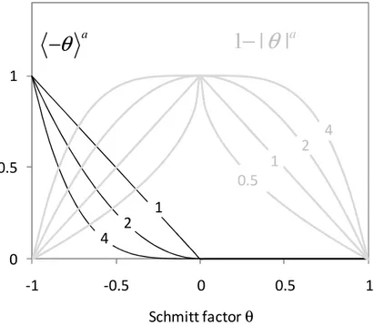
= − = − = − − , (17)

where the parameter a is a constant and p is a material parameter. After this instantaneous redistribution of the three components of the dislocation density, their respective evolutions are governed by Eqs. (12). The influence of parameter a on the heuristic functions utilized in Eq. (17) is shown in Figure 1. Rauch et al. [37] proposed the value a = 2, inferred from extensive experimental investigations [47, 48].

0 0.5 1 -1 -0.5 0 0.5 1 Schmitt factor θ a

θ

−

1 | |

−

θ

a 1 2 4 0.5 1 2 4

Figure 1. Strain-path change heuristic functions and influence of parameter a.

This simple approach is intended to model loading conditions involving one single, abrupt strain-path change. However, general strain paths issued from the numerical simulation of forming processes often do not fall into this particular case:

• The strain path may evolve in a continuous manner between two different modes, rather than abruptly, so that the θ-value measured between two successive time increments will be close to unity and would not detect the overall strain-path change. • Spurious oscillations of the strain path in the vicinity of a uniform value may give the

illusion of instantaneous strain paths significantly different from the average one. • More than one significant strain-path change may occur in material points of sheet

metal during forming.

In order to overcome these limitations, we adopted the strain-path change indicator (SPCI) proposed by van Riel and co-workers [49, 50] instead of Schmitt’s factor in Eqs. (17). This indicator compares the current plastic strain increment to a second-order tensor representative of the plastic strain history, rather than comparing two sequential, instantaneous, plastic strain directions. With this indicator, continuous strain-path changes are still detected,

independently of the strain-increment size. The SPCI ξ is defined as : p p ξ = G G ɺ ɺ ε ε (18)

and the evolution of the second-order tensor G is defined as

(

1

)

p c c = − Gɺ ɺε N G , (19)

where G(0) =0 and

c

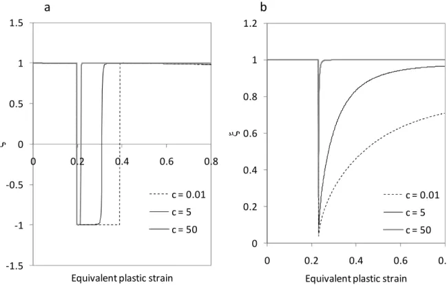
_{is a parameter defining the saturation rate of tensor G. Indeed, when c} increases, the history of strain path arrives earlier at saturation, as illustrated in Figure 2. A

value equal to 5 is taken in the forthcoming simulations [39, 49]. 0 0.2 0.4 0.6 0.8 1 1.2 0 0.2 0.4 0.6 0.8 ξ

Equivalent plastic strain c = 0.01 c = 5 c = 50 -1.5 -1 -0.5 0 0.5 1 1.5 0 0.2 0.4 0.6 0.8 ξ

Equivalent plastic strain c = 0.01 c = 5 c = 50

a

b

Figure 2. Evolution of the van Riel strain-path-change indicator

ξ

_{during (a) reverse and (b)} orthogonal loading sequences.

A strain-path change is detected when the SPCI significantly deviates from unity (e.g. is smaller than a threshold value) and Eqs. (17) are used to re-initialize the three components of the dislocation density. Afterwards, the detection of subsequent strain-path changes may be inhibited until the end of the simulation. Alternatively, the strain-path change detection may be reactivated once the loading mode becomes quasi-monotonic (the SPCI approaches unity). For all of the simulations performed in the current investigation, the rule (17) is adopted to decompose the dislocation density after a strain-path change, where the Schmitt factor θ is replaced by the SPCI

ξ

.

2.3 Material parameters and required identification procedure

One of the strengths of the adopted modeling is the physical meaning of several of its material parameters, which allowed a simplified identification procedure. The parameters of the

constitutive model fall within several categories in terms of physical significance, as depicted in Table 1. A first category of parameters ( , , , , ,M

α

G b

ρ

₀ k_HP) are directly related to the crystallographic structure of the material, their values (e.g., for steels) being available in the literature (see Table 2). The physically-based parameters k1, k2, k3, λ, and n0 describe the

hardening behavior and are specific to a family of materials. They were identified using strain-path change mechanical tests. The full range of tests utilized for the identification comprises a tensile test, a shear test, three reverse shear tests, and an orthogonal test

these tests were performed in the rolling direction. For the needs of the current study, these parameters were identified once for all for the IF steels, and once for all for the DP steels, using the experimental results from a previous study [24]. Finally, material parameters related to microstructure were identified for each material using chemical composition and analysis of scanning electron microscopy (SEM) observations. It is noteworthy that these metallurgical analyses are not required for classical macroscopic models, and some of them may also be tedious and time-consuming. From the perspective of industrial application, the advantage of replacing monotonic (tensile, shear) and sequential (reverse, orthogonal) mechanical tests with metallurgical measurements is an overall cost and time reduction, along with the benefit of the standardization of parameter determination, avoiding the use of inverse methods. The studied materials and the corresponding parameters are summarized in the next section, along with deep drawing experiments performed on the same steel sheets in order to explore the predictive capability of the model.

Table 1. The different types of parameters of the constitutive model and their corresponding identification procedure.

Parameters Identification range

Identification procedure, required experiments

0

, , , , , _HP

M

α

G b

ρ

k For each family of

steels (IF/DP) From literature.

1, , , , ,2 3 0

k k k λ n p For one material in

the family (IF/DP) 1 tensile test, 1 shear test, 3 reverse shear tests, 1 orthogonal test (tensile + shear). [Mn],…

For each material

Chemical composition analysis.

, ,

F M M

D D V Micrographs.

F, G, H, L, M, N For IF steels: 3 tensile tests at 0°, 45°, 90°. _{For DP steels: von Mises yield function.}

Table 2. Material parameters determined once for all, based on literature (see, e.g., [53] or [54] for the values of parameter kHP).

Material parameters IF steels DP steels

M 3.14 3.14

α

0.4 0.4

[

MPa

]

G

80000 80000

[ ]

m

b

2.46 10× −10 2.46 10_× −10 2 0 m ρ _ − _   10 12 _{12 13} 0 10 ; 0 10 F M ρ = ρ = MPa mm HP k _  

16.5

20

3. Application to the cross-die deep drawing test

The purpose of this study is to investigate the potential benefits of the modeling approach described in Section 2 for the accurate numerical simulation of sheet forming processes, while reducing significantly the effort on parameter identification. The cross-die deep drawing test has been selected for the analysis and a number of fourteen sheet steels were investigated. These were both IF and DP steels with relatively large ranges of grain size, martensite volume fraction, chemical composition and initial crystallographic texture. This section presents the material data and the deep drawing experiments. The constitutive model was implemented in the finite element code Abaqus/explicit as a user material routine, in order to allow for the numerical simulation of the deep drawing processes and to assess the accuracy of both the model and its selective parameter identification procedure.

3.1 Materials and parameters

Single-phase IF steels and dual-phase steels were selected for the investigation. As shown in Table 3, the sheet thickness varied between 0.7 mm and 1.78 mm for the IF steels, and

between 0.7 and 2.2 mm for the DP steels. The use of phenomenological elasto-plastic models classically available in finite element simulation codes would require the model parameters to be identified for each of these materials. In the current investigation, only the grain size and martensite volume fraction (when applicable) were determined for each material using

micrographs. Additionally, tensile tests were performed in three directions of the sheet’s plane (at 0°, 45° and 90° with respect to the rolling direction) for the IF steels in order to account for their anisotropy. The material parameters identified with this simplified analysis are summarized in Table 4. Concerning the anisotropy coefficients, a linear interpolation was further performed as they have been shown to vary almost linearly with the ferrite grain size [27, 39]. The calculation of the linear law parameters based solely on chemical composition and microstructure is still under research and in the current analysis these parameters were determined experimentally. However, the accuracy of using such linearly-interpolated anisotropy parameters was also addressed in the current study.

The six remaining parameters, namely k1, k2, k3, λ, n0 and p, which enter the hardening laws (12)–(14), were determined for a single IF steel (IF I) and for a single DP steel (DP II), the other materials being available for validation purposes. This is a time-consuming step requiring non-classical sequential experimental tests. The experiments used for the

identification were a tensile test, a shear test, three reverse shear tests with shear pre-strains between 0.1 and 0.3, and a shear test following a tensile pre-strain of 0.1 (orthogonal test), all of these tests being performed in the rolling direction. However, no such a test was performed for the current analysis since the required experimental data was taken from previous studies [24]. The six parameters were identified simultaneously, using a standard minimization routine of Matlab. In the objective function, which measures the gap between the predicted and experimental stress–strain curves in a least-squares sense, all of the experiments had the same weight except for the orthogonal test, whose weight was five times larger. The identified parameters are summarized in Table 5.

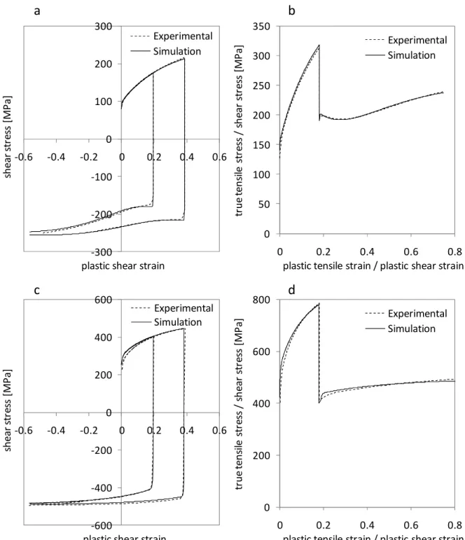
Figure 3 illustrates the accuracy of the model’s predictions during one-element simulations of abrupt strain-path changes for the two materials that served for the identification. The

implementation of the constitutive model for arbitrary loading sequences (i.e. including repeated elastic unloading and plastic reloading sequences).

Table 3. IF and DP steels process information. CR and HR stand for cold rolled and hot rolled, respectively. Material Rolling condition Thickness [mm] Material Rolling condition Thickness [mm] IF I CR 0.7 DP I (DP 450) CR 2 IF II CR 0.8 DP II (DP 600) CR 0.7 IF III CR 0.7 DP III (DP 600) HR 2.2 IF IV CR 0.8 DP IV (DP 600) CR 1.82 IF V HR 1.78 DP V (DP 800) CR 1.96 IF VI CR 1.62 DP VI (DP 800) CR 1.5 DP VII (DP 1000) CR 2 DP VIII (DP 1000) CR 1.4

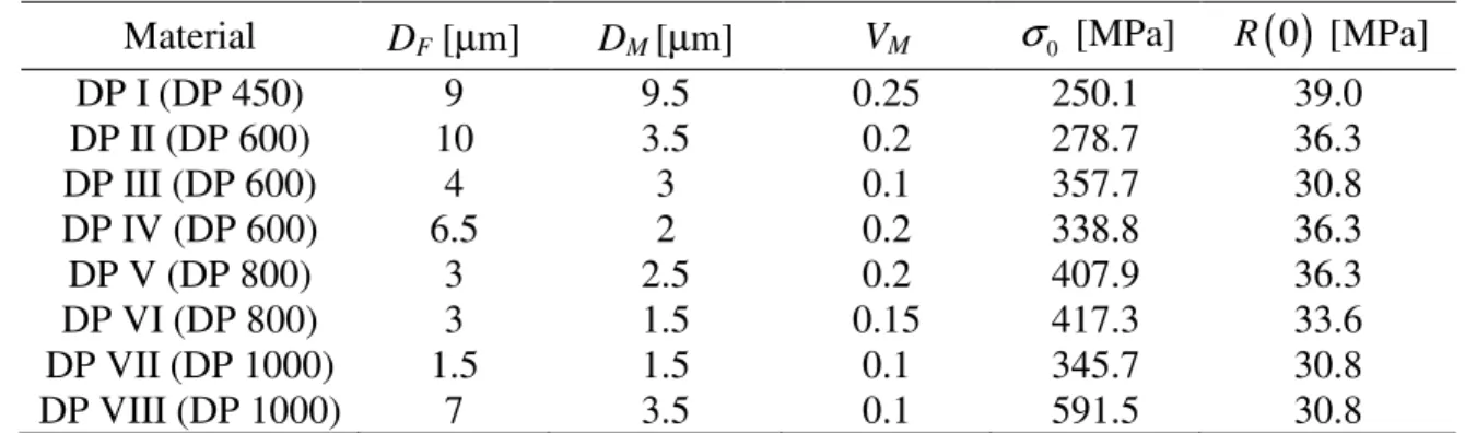
Table 4. Microstructure-based material parameters for the studied materials. Parameters F, G, H, L, M, and N enter Hill’s quadratic yield surface; DF and DM are the ferrite and martensite

grain sizes, respectively; VM is the martensite volume fraction; σ0 and R

( )

0 are the two

terms of the initial yield stress. a) IF steels

Material DF

[µm]

Experimental values Linear interpolation _σ0 [MPa]

( )

0 R [MPa] F G H N F G H N IF I 25 0.25 0.32 0.68 1.42 0.27 0.28 0.72 1.19 96.3a 24.7 IF II 25 - - - - 0.27 0.28 0.72 1.19 88.3 a 24.7 IF III 22 0.27 0.28 0.72 1.23 0.28 0.3 0.70 1.23 153.6 24.7 IF IV 15 0.34 0.35 0.65 1.13 0.34 0.38 0.62 1.34 223.0 24.7 IF V 10.5 0.45 0.54 0.46 1.50 0.40 0.49 0.51 1.50 235.8 24.7 IF VI 8 0.41 0.61 0.39 1.79 0.45 0.64 0.36 1.65 275.3 24.7 Parameters L and M are set equal to N for all of the materials.

a _{The chemical composition was not available for IF I and II, thus the initial yield stress was} determined based on tensile tests.

b) DP steels

Material DF [µm] DM [µm] VM σ0 [MPa] R

( )

0 [MPa]

DP I (DP 450) 9 9.5 0.25 250.1 39.0 DP II (DP 600) 10 3.5 0.2 278.7 36.3 DP III (DP 600) 4 3 0.1 357.7 30.8 DP IV (DP 600) 6.5 2 0.2 338.8 36.3 DP V (DP 800) 3 2.5 0.2 407.9 36.3 DP VI (DP 800) 3 1.5 0.15 417.3 33.6 DP VII (DP 1000) 1.5 1.5 0.1 345.7 30.8 DP VIII (DP 1000) 7 3.5 0.1 591.5 30.8

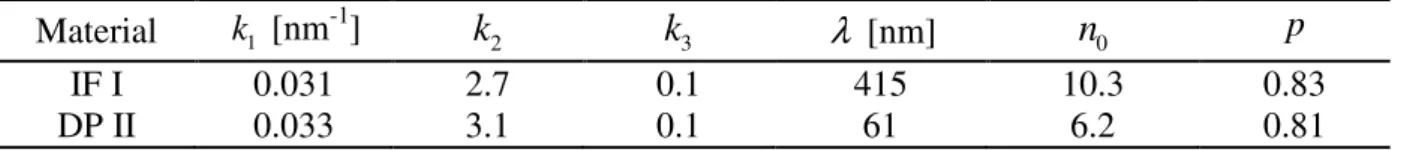
Table 5. Material parameters for IF I steel and DP II steel, identified using mechanical tests: a tensile test, a shear test, three reverse shear tests, and an orthogonal test consisting in a tensile pre-strain followed by a shear test in the same direction. All of these tests were performed in the rolling direction [24]. The parameters identified for IF I were subsequently used for all of the simulations concerning IF steels, and the parameters identified for DP II were used for all of the simulations concerning DP steels.

Material k1 [nm -1_] 2

k

k

₃ λ [nm]

n

0 p IF I 0.031 2.7 0.1 415 10.3 0.83 DP II 0.033 3.1 0.1 61 6.2 0.81

0 200 400 600 800 0 0.2 0.4 0.6 0.8 tr u e t e n si le s tr e ss / s h e a r st re ss [ M P a ]

plastic tensile strain / plastic shear strain Experimental Simulation -600 -400 -200 0 200 400 600 -0.6 -0.4 -0.2 0 0.2 0.4 0.6 sh e a r st re ss [ M P a ]

plastic shear strain

Experimental Simulation 0 50 100 150 200 250 300 350 0 0.2 0.4 0.6 0.8 tr u e t e n si le s tr e ss / s h e a r st re ss [ M P a ]

plastic tensile strain / plastic shear strain Experimental Simulation -300 -200 -100 0 100 200 300 -0.6 -0.4 -0.2 0 0.2 0.4 0.6 sh e a r st re ss [ M P a ]

plastic shear strain

Experimental Simulation

a

b

c

d

Figure 3. Accuracy validation of the model and its numerical implementation for IF I (top) and DP II (bottom) steels during two-step strain paths. Left: simple shear in rolling direction following simple shear pre-strain in the opposite direction up to shear strain values of 0.2 and 0.4. Right: simple shear in rolling direction following tensile tests in the same direction up to a tensile true strain of 0.18.

The experiments shown in Figure 3 have served for the parameter identification. Figure 4a shows the model predictions for two shear experiments that did not serve for the identification, for the IF I steel sheet. As expected, the accuracy is relatively lower as compared to the

previous figure. One source of inaccuracy comes from the use of Hill’s quadratic yield criterion to estimate the initial yield stresses; its validity can be evaluated from the fit obtained at low plastic strains. Another source of inaccuracy is due to the use of the same hardening equations in all directions, and to the absence of the texture evolution effect.

Accordingly, the gap between predictions and experiments is increasing with the plastic strain. The maximum error, at 0.45 shear strain, is of 2.2% with respect to the experiment at 45°, and 4.7% with respect to the experiment at 135°. It is noteworthy that the difference between these two experiments illustrates the material’s deviation from orthotropy, and cannot be accounted for with the selected model. Figure 4b shows more experimental curves from shear tests at different orientations in the plane of the sheet. This figure illustrates the relatively weak anisotropy of the materials used in the current study. Consequently, the conclusions of this analysis mainly apply to weakly anisotropic steel sheets; the extension to other classes of sheet metals, and to more anisotropic ones, may require further investigation. Of course, these limitations are common to all of the macroscopic models commonly used in industrial finite element simulations. 0 50 100 150 200 0 0.1 0.2 0.3 0.4 0.5 sh e a r st re ss [ M P a ]

plastic shear strain Experiment, 135° Experiment, 45° Simulation 0 50 100 150 200 0 0.1 0.2 0.3 0.4 0.5 sh e a r st re ss [ M P a ]

plastic shear strain Shear, 0° Shear, 45° Shear, 90° Shear, 135° Shear, 150° Tensile, 0°, scaled

a

b

Figure 4. Illustration of the model accuracy for the IF I steel: (a) experimental and simulated simple shear response for a shear direction oriented at 45° and at 135° with respect to the rolling direction; (b) experimental simple shear response for various orientations of the shear direction, along with a tensile test response in the rolling direction. The tensile test curve is scaled with a factor of 1 3, corresponding to a von-Mises-type equivalence.

Carvalho-Resende et al. [27, 39] present and discuss in detail the experiments and the

accuracy of such rheological predictions for all of the materials in Table 3. Figures 5a and 5b compare the predictions of reverse shear tests to experiments for two IF and two DP steels, respectively, which exhibit the lowest and the highest yield strength in each category. The errors are the largest for IF VI and for DP VIII, respectively. It is noteworthy that the sheet steels used for the identification had relatively low yield strengths, which partly explains this result. On the other hand, larger ranges of tensile plastic strains can be attained for lower-strength materials, which is beneficial for the parameter identification accuracy. Consequently, the choice of the particular material that is used for the identification has a non-trivial

influence on the final results. Eventually, the proposed approach allowed for a first approximation of the material response for several materials, in a wide range of yield strengths, with very few experimental inputs – which was its principal expected benefit.

-400 -300 -200 -100 0 100 200 300 400 -0.3 -0.2 -0.1 0 0.1 0.2 0.3 sh e a r st re ss [ M P a ]

plastic shear strain Experiment Simulation -800 -600 -400 -200 0 200 400 600 800 -0.3 -0.2 -0.1 0 0.1 0.2 0.3 sh e a r st re ss [ M P a ]

plastic shear strain Experiment Simulation

a

b

Figure 5. Experimental and predicted reverse shear tests for the IF and DP sheet steels

exhibiting the smallest and the largest yield strength in their category, respectively. Left: IF II and IF VI. Right: DP I and DP VIII. The shear pre-strain is close to 0.2 in all cases.

3.2 Cross-die test experiments and numerical simulation

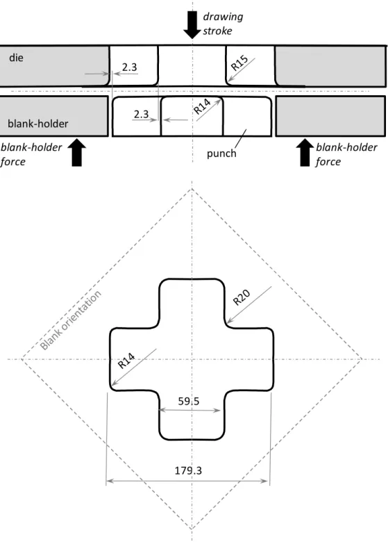
The “cross-die” deep drawing test, originally designed by the automotive industry as a press-shop formability test for aluminum sheets, is known to reproduce most of the industrially-relevant strain paths encountered in deep drawing, i.e. tensile, plane strain, shear and biaxial loading modes (see, e.g., [55]). This test is regularly used by carmakers as a validation tool for hardening laws before simulating industrial parts. In the current investigation, cross-die deep drawing tests were performed on an 800 kN hydraulic press at Renault. The punch, the blank holder and the die are made of uncoated hardened tool steel. The blanks were lubricated with grease and Teflon on both sides. Figure 6 shows the main geometrical parameters of the tools; the same set of tools was used for all of the tests. The die and punch radii are 20 and 14 mm, respectively. The drawing stroke and blank size were different for each material; their values are summarized in Table 6. Different blank sizes and press strokes are selected in order to reach the largest strain values acceptable for each material, without inducing any strain localization. In all cases, the initial blank was square; its orientation with respect to the tools is shown in Figure 6. The blank holding force was 450 kN for all of the trials.

179.3 59.5 2.3 blank-holder force blank-holder force drawing stroke die blank-holder punch 2.3

Figure 6. Sketch of the deep drawing tooling used for the cross-die deep drawing test experiments. The die geometry respects a clearance of 2.3 mm along the transverse contour with respect to the punch.

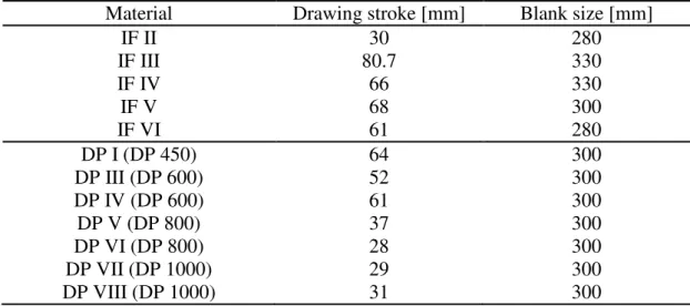
Table 6. Drawing depth and blank size for the different materials of the study.

Material Drawing stroke [mm] Blank size [mm]

IF II 30 280 IF III 80.7 330 IF IV 66 330 IF V 68 300 IF VI 61 280 DP I (DP 450) 64 300 DP III (DP 600) 52 300 DP IV (DP 600) 61 300 DP V (DP 800) 37 300 DP VI (DP 800) 28 300 DP VII (DP 1000) 29 300 DP VIII (DP 1000) 31 300

After the tests, the material thinning was measured along three directions (i.e. rolling direction RD, diagonal direction DD, transverse direction TD) as depicted in Figure 7, by ultrasonic method. However, the thickness distributions along RD and TD were very close, and only the values recorded along the RD directions are reported hereafter. Thickness measurement accuracy was of ±0.01mm. Measurements are done every 10 mm on the outer surface of the deformed configuration, starting from the center of the part. For some of the materials, the blanks have been marked with a 2-mm dotted pattern and strain distribution analyses have been performed with the ARGUS strain measurement system.

RD

DD

TD

Figure 7. Specimen after cross tool forming operation. The thickness measurements were performed along the three directions RD (rolling direction), DD (diagonal direction) and TD (transverse direction).

The FE simulation is performed using the dynamic explicit code Abaqus/Explicit with a user-defined material routine VUMAT incorporating the model described in Section 2. According to mesh sensitivity investigations of the thickness and strain distributions [56, 57], the blank is meshed with 17298 (93×93×2) reduced-integration linear hexahedra (C3D8R). The tools are considered rigid. Due to the symmetry, only one quarter of the geometry is meshed as shown in Figure 8.

Die

Blank

Blank holder

Punch

Figure 8. Cross-die test FE model.

4. Results and discussion

4.1 Typical strain paths and corresponding dislocation density evolution

Sheet metal forming processes often involve complex loading sequences. For instance, most deep drawing processes involve bending-unbending sequences when the sheet passes over the die radius. The modeling of the reverse loading behavior of the material directly influences the springback predictions [23, 58]. Multi-step drawing processes often involve

quasi-orthogonal strain paths [59]. The SPCI adopted in this model can be used to determine the strain-path changes that occur during the cross-die deep drawing test, as well as their

amplitudes. Figure 9a shows that the cross-die test induces both orthogonal and reverse strain paths in three different regions of the part. As the SPCI evolution in the upper and the lower layers of the sheet was roughly the same, its evolution was only investigated for the upper one. The SPCI evolution was further monitored for seven material points located in different areas of the blank (see Figure 9b) in the vicinity of the previously detected zones A, B and C. The evolution plots shown in Figure 10 confirm that quasi-orthogonal strain-path changes occur at points 1 and 6 (i.e.

ξ

reaches a minimum value close to 0 and gradually returns to 1 in zones A and C), quasi-reverse strain-path change at points 3 and 4 (i.e.

ξ

reaches a minimum value close to -1 and gradually returns to 1 in zone B) and quasi-monotonic strain path at points 2, 5 and 7 (i.e.

ξ

remains close to 1). In all of these material points, the strain-path changes occur after a punch travel that is greater than 35 mm. Indeed, strain-path changes at points 1 and 6 occur when the punch displacement is around 35 mm while for points 3 and 4 they take place approximately at 40 and 50 mm, respectively. It is noteworthy that at each of the material points that were investigated, at most one single strain-path change was recorded, which occurred relatively suddenly. This observation supports the application of the scalar decomposition of the dislocation density as a simple and effective means to describe the transient hardening behavior even during continuous, one-step drawing processes.

A B C 1 2 3 4 5 6 7

b

a

ξ

Figure 9. a) Distribution of the SPCI at the end of the drawing process for IF I and b) material points used for the investigation of SPCI evolution.

-1 -0.5 0 0.5 1 0 10 20 30 40 50 60 ξ Punch displacement [mm] Point 2 -1 -0.5 0 0.5 1 0 10 20 30 40 50 60 ξ Punch displacement [mm] Point 1 0 10 20 30 40 50 60 Punch displacement [mm] Point 5 0 10 20 30 40 50 60 Punch displacement [mm] Point 7 0 10 20 30 40 50 60 Punch displacement [mm] Point 3 0 10 20 30 40 50 60 Punch displacement [mm] Point 4 0 10 20 30 40 50 60 Punch displacement [mm] Point 6

Point 1, zone A Point 6, zone C Point 3, zone B Point 4, zone B

Point 2 Point 5 Point 7

Figure 10. Evolution of the SPCI at different material points, emphasizing quasi-orthogonal strain-path change at points 1 and 6 (zones A and C), quasi-reverse strain-path change at points 3 and 4 (zone B) and quasi-monotonic strain path at points 2, 5 and 7.

The impact of the strain-path change events on hardening is taken into account in the proposed model solely through the evolution of the dislocation density and its components. The evolution of the total dislocation density

ρ

for material points 1, 3, 4, and 6 is

represented in Figure 11. The largest amounts of work hardening are recorded at the middle points of the outer edges of the blank, where the draw-in is the largest according to the die geometry, and on the drawn wall of the part – close to the zones B and C identified previously. Although the authors found no experimental dislocation density measurements for mild steels drawn parts in the literature, the order of magnitude (10 ...1012 13m-2) corresponds to those experimentally observed in monotonic tensile tests for similar steel grades [60].

Figure 12 shows the evolution of the three components of the dislocation density. At the values of punch stroke where strain-path changes were identified in Figure 10, a drop of the forward dislocation density ρF occurs that reveals the apparition of the reverse or of the

latent dislocation densities ρ_R and ρ_L, respectively, for the different material points, according to the rule (17). At points 1 and 6, a quasi-orthogonal strain path is observed at positive values of the SPCI, thus without activation of the “reverse” dislocation density. In

turn, the SPCI takes negative values at material points 3 and 4 (zone B) thus activating both “latent” and “reverse” components.

Of course, these local events occur independently of each other at different values of punch travel; consequently, their effect is not visible on the load-displacement plot, in contrast e.g. with the case of homogeneous mechanical tests involving abrupt strain-path changes. In turn, the local behavior may affect significantly the final predictions of springback or formability, provided that the strain-path change occurs after a sufficient amount of pre-strain [25, 26, 61]. Figure 13 reveals that the strain-path change occurs at cumulated plastic strain amounts of 0.04, 0.05, 0.35, and 0.3 at material points 1, 3, 4, and 6, respectively. Hence, due to the fact that little strain is accumulated, typical strain-path change effects for mild steels such as work softening in element 1 and work hardening stagnation in element 3 may be minor. On the other hand, the effect of strain-path change in elements 4 and 6 can be sufficiently important to affect the results of the finite element simulation. The effects of strain-path changes at the end of the process were assessed and are presented in the next section. In order to investigate the additional effect due to the description of the transient behavior after orthogonal strain-path change (observed in regions B and C near the die radius contour), the proposed model is first compared to a simpler phenomenological model in the context of the cross-die deep drawing simulation. 0 2 4 6 8 10 0 10 20 30 40 50 60 To ta l d is lo ca ti o n d e n si ty ρ [1 0 1 3m -2] Punch displacement [mm] Element 1 Element 3 Element 4 Element 6 1 3 6 4 ρ[mm-2_]

Figure 11. Distribution of the total dislocation density at 60-mm punch displacement (left) and its evolution (right) in the cross-die deep drawing test for IF I.

0 2 4 6 8 10 0 10 20 30 40 50 60 La te n t d is lo ca ti o n d e n si ty ρL [1 0 1 3m -2] Punch displacement [mm] Element 1 Element 3 Element 4 Element 6 0 2 4 6 8 10 0 10 20 30 40 50 60 R e v e rs e d is lo ca ti o n d e n si ty ρR [1 0 1 3m -2] Punch displacement [mm] Element 1 Element 3 Element 4 Element 6 0 2 4 6 8 10 0 10 20 30 40 50 60 F o rw a rd d is lo ca ti o n d e n si ty ρF [1 0 1 3m -2] Punch displacement [mm] Element 1 Element 3 Element 4 Element 6 1 3 6 4 3 4 1 3 6 4 ρF[mm-2] ρR[mm-2] ρL[mm-2]

Figure 12. Distribution of the forward (top), reverse (middle) and latent (bottom) dislocation densities at 60-mm punch displacement (left) and their evolutions (right) in the cross-die deep drawing test for IF I.

0 0.1 0.2 0.3 0.4 0.5 0.6 0 10 20 30 40 50 60 E q u iv a le n t p la st ic s tr a in Punch displacement [mm] Element 1 Element 3 Element 4 Element 6 1 4 3 6 ε

Figure 13. Equivalent plastic strain distribution at 60-mm punch displacement (left) and its evolution (right) in the cross-die deep drawing test for IF I.

4.2 Comparison with a classical isotropic-kinematic hardening model

In order to evaluate the effect of strain-path change on the results of cross-die test, simulations were performed with a classical isotropic-kinematic hardening model and with the proposed model. The so-called Chaboche model adopted as reference is described by Eq. (7) for the kinematic hardening, and the isotropic hardening is governed by the rate equation

(

)

R sat

Rɺ =C R −R εɺ, (20)

where CX, Xsat, CR, and Rsat are constant. These parameters were identified in order to fit

closely the prediction of monotonic and reverse shear tests up to large strains; a very good fit could be obtained since the classical model can be viewed as a particular case of the proposed model. The resulting parameters are summarized in Table 7.

Table 7. Material parameters of the classical hardening model, fitted for the mild steel IF I [24].

0

σ [MPa] CR Rsat [MPa] CX Xsat [MPa]

The cross-die drawing test was simulated using the two models, leaving unchanged all of the other numerical parameters. The computing time required for the proposed model was about 20% larger as compared to the classical model. Figure 14 compares the thickness distributions predicted along the rolling and the diagonal directions by the two models. The results

obtained for 30 mm of punch travel were similar between the two models in both directions. This is consistent with the fact that no strain-path change was observed at punch strokes smaller than 35 mm. However, the results of the two models significantly differed at a punch stroke of 60 mm, with the classical model underestimating the maximum thinning in the part. This preliminary result shows that such transient and local differences in the constitutive modeling may have an influence on industrial process simulations, e.g. in terms of thickness distribution. Consequently, the proposed model was further confronted to experimentally determined thickness distributions for the same deep drawing test, and for several IF and DP steel grades.

0.6 0.7 0.8 0.9 1 0 50 100 150 th ic k n e ss [ m m ] location [mm] Classical model Proposed model 0.6 0.7 0.8 0.9 1 0 50 100 150 200 th ic k n e ss [ m m ] location [mm] Classical model Proposed model 0.6 0.7 0.8 0.9 1 0 50 100 150 th ic k n e ss [ m m ] location [mm] Classical model Proposed model 0.6 0.7 0.8 0.9 1 0 50 100 150 200 th ic k n e ss [ m m ] location [mm] Classical model Proposed model Diagonal direction 30 mm punch displacement Diagonal direction 60 mm punch displacement Rolling direction 30 mm punch displacement Rolling direction 60 mm punch displacement

Figure 14. Thickness distribution for the cross-die tests along DD and RD at 30-mm punch displacement, before the strain-path changes take place (top), and at the end of the process corresponding to 60-mm punch displacement (bottom).

4.3 Experimental validation of predicted thickness distributions

Finally, the cross-die deep drawing test was used to evaluate the predictive capacity of the proposed approach. The experimental test was performed for five IF steels and seven DP steels as summarized in Table 6 and the experimental thickness distributions were measured. The material parameters were identified for the IF I and DP II sheets. These two materials have been investigated during a previous study [24] and they were not part of the set of materials used for the drawing experiments. Only the grain size, volume fraction and chemical composition served to adjust the model to each of these materials.

Figure 15 shows the experimental and predicted thickness distributions along the rolling direction for the five IF steel sheets on which deep drawing tests were performed. The

predictions lay very close to the experimental values for all of the materials. The results along the diagonal direction followed the same trend. In particular, the minimum value of the thickness along the selected material line is well predicted, which is critical for the correct assessment of the overall formability. Additionally, the in-plane strain distribution was measured for one of the sheets (IF VI) at the end of the drawing test. Figure 16 compares the “strain signature” predicted for this part to the experimental one and a satisfactory agreement was observed. This figure also shows that the drawing process was conducted very close to the occurrence of necking, for a discriminating confrontation.

The same comparison procedure was repeated for the seven DP steels designated in Table 6. The blank size was the same for all of the drawing tests on DP steels. However, due to the large differences in the ultimate yield strength for these materials (according to the different grain sizes and martensite volume fractions), different drawing depths were attained. In spite of these large variations, the predictions of the thickness distributions summarized in Figure 17 indicate a good overall accuracy.

0.6 0.7 0.8 0.9 1 1.1 1.2 1.3 0 50 100 150 200 re la ti v e t h ic k n e ss t /t0 location [mm] Experimental Proposed model 0 50 100 150 200 location [mm] Experimental Proposed model 0 50 100 150 200 location [mm] Experimental Proposed model 0.6 0.7 0.8 0.9 1 1.1 1.2 1.3 0 50 100 150 200 re la ti v e t h ic k n e ss t /t0 location [mm] Experimental Proposed model 0 50 100 150 200 location [mm] Experimental Proposed model IF II IF III IF IV IF V IF VI

Figure 15. Experimental and predicted thickness distributions for cross-die tests along RD (rolling direction) at the end of the process, for the five IF steels subjected to the deep drawing experiments. Symbols t and t0 designate the final and the initial thickness of each sheet, respectively.

0 0.075 0.15 0.225 0.3 0.375 0.45 0.525 0.6 -0.6 -0.5 -0.4 -0.3 -0.2 -0.1 0 0.1 0.2 0.3 m a jo r st ra in minor strain Predicted strain distribution Experimental FLD

Figure 16. Strain distribution after the cross-die deep drawing tests predicted with the proposed model (top) and experimentally obtained (bottom) for IF VI.

0.6 0.7 0.8 0.9 1 1.1 1.2 1.3 0 50 100 150 200 re la ti v e t h ic k n e ss t /t0 location [mm] Experimental Proposed model 0 50 100 150 200 location [mm] Experimental Proposed model 0.6 0.7 0.8 0.9 1 1.1 1.2 1.3 0 50 100 150 200 re la ti v e t h ic k n e ss t /t0 location [mm] Experimental Proposed model 0 50 100 150 200 location [mm] Experimental Proposed model 0.6 0.7 0.8 0.9 1 1.1 1.2 1.3 0 50 100 150 200 re la ti v e t h ic k n e ss t /t0 location [mm] Experimental Proposed model 0 50 100 150 200 location [mm] Experimental Proposed model 0 50 100 150 200 location [mm] Experimental Proposed model DP I (450) DP III (600) DP IV (600) DP V (800) DP VI (800) DP VII (1000) DP VIII (1000)

Figure 17. Experimental and predicted thickness distributions for cross-die tests along RD (rolling direction) at the end of the process, for the seven DP steels subjected to the deep drawing experiments. Symbols t and t0 designate the final and the initial thickness of each sheet, respectively.

5. Summary and discussion

A recently developed elasto-plastic model [27, 39] was implemented in a commercial finite element code for sheet metal forming applications. Scalar, dislocation-density-like variables were used to account for the transient phenomena after strain-path changes, which proved very efficient compared to other macroscopic models and carrying more physical signification – although this conveys only a limited part of the predictive richness of crystal plasticity models due to the use of a macroscopic, non-evolving yield surface. The main strength of this model is to significantly simplify the parameter identification requirements. A full series of mechanical tests for the identification is only required for one member of a given family of materials (e.g., IF steels and DP steels). Then, the model adjusts to each individual material using only the chemical composition, the grain size and the volume fraction of the second phase, if any. In order to investigate the predictive potential of this approach, experimental cross-die deep drawing tests were performed on five IF steels and seven DP steels. The hardening model for each of these materials was set without performing mechanical tests; the microstructure data and chemical composition were combined with experimental data

available for an arbitrary IF steel and DP steel.

The strain-path changes induced by the cross-die deep drawing test in various areas of the part were investigated. Only one single strain-path change was detected at each material point, if any; these occurred in three zones of the part, located close to the punch or die radius. The comparison with a classical isotropic-kinematic hardening model showed that the

consideration of the strain-path changes in the material model modifies the overall forming prediction for this test in terms of thickness distributions.

The comparison of the predicted thickness distributions with the experimental ones showed very good accuracy for the IF and the DP steels, although the sheet materials were very different in terms of strength and thickness. Consequently, the proposed approach could be an efficient and accurate alternative for the numerical simulation of industrial sheet metal

forming processes, reducing significantly the cost of the parameter identification. The

implemented strain-path change indicator can be used with any constitutive model in order to quantify the presence and importance of strain-path changes in a simulation and evaluate if the use of simpler constitutive models is sufficient for a given process.

At this stage, tensile tests were performed for the identification of the anisotropy parameters for the IF steels, which were further approximated by a linear interpolation in terms of the ferrite grain size. This interpolation proved accurate and future work should be dedicated to the determination of the anisotropy parameters based solely on microstructure and chemical composition, and to their combination with non-quadratic yield surfaces. Future investigations are required to assess the accuracy of the proposed approach for other part geometries and sheet steels. In particular, the two materials that served for the sequential mechanical tests were not available for the deep drawing experiments; a more complete validation would consist in applying the entire testing / simulation sequence to selected materials, from the characterization step to the forming experiments. The choice of a particular material for the identification, out of a given class of materials, may also have an impact on the results. Materials with relatively low strength within their category would allow, in general, for a larger range of tensile plastic strains, with a potentially beneficial influence on the

identification accuracy. The current results suggest that the proposed approach can be used to estimate the material parameters for sheet steels from the same class (IF or DP) significantly different from the reference material used for the complete parameter identification (strength ratio up to two, grain-size ratio up to three). The possible extension of this approach to other sheet metals, with different strengthening mechanisms, is under investigation.

Acknowledgements

This research has been performed within a project funded by Renault. The authors gratefully acknowledge Renault for its financial support.

References

[1] Taylor G I 1934 Proceedings of Royal Society of London A 145 362-387 [2] Kocks U F and Mecking H 2003 Progress in Materials Science 48 171-273 [3] Rauch E F, Gracio J J and Barlat F 2007 Acta Materialia 55 2939-2948 [4] Sinclair C W, Poole W J and Bréchet Y 2006 Scripta Materialia 55 739-742 [5] Van Houtte P, Li S, Seefeldt M and Delannay L 2005 International Journal of

Plasticity 21 589-624

[6] Berveiller M and Zaoui A 1978 Journal of the Mechanics and Physics of Solids 26 325-344

[7] Molinari A, Canova G R and Ahzi S 1987 Acta Metallurgica 35 2983-2994 [8] Lebensohn R A and Tomé C 1993 Acta Metallurgica et Materalia 41 2611-2624 [9] Bate P 1999 Philosophical Transactions of the Royal Society A: Mathematical,

Physical and Engineering Sciences 375 1589-1601

[10] Beaudoin A J, Mathur K K, Dawson P R and Johnson G 1993 International Journal of Plasticity 19 833-860

[11] Raabe D and Roters F 2004 International Journal of Plasticity 21 339-361 [12] Böhlke T, Haus U-U and Schulze V 2006 Acta Materialia 54 1359-1368

[13] Böhlke T, Risy G and Bertram A 2006 Modelling and Simulation in Materials Science and Engineering 14 365-387

[14] Habraken A M and Duchêne L 2004 International Journal of Plasticity 21 1525-1560 [15] Dawson P R, Boyce D E, Hale R and Dukrot J P 2005 International Journal of

Plasticity 21 251-283

[16] Van Houtte P and Van Bael A 2004 International Journal of Plasticity 20 1505-1524 [17] Van Houtte P, Yerra S K and Van Bael A 2009 International Journal of Plasticity 25

332-360

[18] Bertram A, Böhlke T and Risy G 2008 International Journal of Material Forming 1 209-212

[19] Plunkett B, Cazacu O, Lebensohn R A and Barlat F 2007 International Journal of Plasticity 23 1001-1021

[20] Kraska M, Doig M, Tikhorimov D, Raabe D and Roters F 2009 Computational Material Science 46 383-392

[21] Gawad J, Van Bael A, Eyckens P, Samaey G, Van Houtte P and Roose D 2012 Computational Materials Science DOI:dx.doi.org/10.1016/j.commatsci.2012.05.056 [22] Teodosiu C and Hu Z 1995 Numiform’95 Proceedings p 173-182

[23] Geng L, Shen Y and Wagoner R H 2002 International Journal of Plasticity 18 743-767

[24] Haddadi H, Bouvier S, Banu M, Maier C and Teodosiu C 2006 International Journal of Plasticity 22 2226-2271

[25] Bouvier S, Alves J L, Oliveira M C and Menezes L F 2005 Computational Material Science 32 301-315

[26] Haddag B, Balan T and Abed-Meraim F 2007 International Journal of Plasticity 23 951-979

[27] Carvalho-Resende T, Bouvier S, Abed-Meraim F, Balan T and Sablin S-S 2012 Dislocation-based model for the prediction of the behavior of b.c.c. materials - Grain size and strain path effects Internal report

[28] Simo J C and Hughes T J R 1998 Computational Inelasticity, Series "Interdisciplinary Applied Mathematics" (Berlin: Springer)

[29] Hughes T J R 1984 Numerical implementation of constitutive models: rate-independent deviatoric plasticity, in Theoretical foundation for large-scale computations for nonlinear material behavior, Nemat-Nasser S, Asaro R J and Hegemier G A Editors (Dordrecht, The Netherlands: Martinus Nij Publishers) [30] Xiao H, Bruhns O T and Meyers A 1998 International Journal of Solids and

Structures 35 4001-4014

[31] Ponthot J-P 2002 International Journal of Plasticity 18 91-126

[32] Arsenlis A and Parks D M 2002 Journal of the Mechanics and Physics of Solids 50 1979-2009

[33] Cheong K-S and Busso E P 2004 Acta Materialia 52 665-5675 [34] Ma A, Roters F and Raabe D 2006 Acta Materialia 54 2169-2179 [35] Gao H and Huang Y 2003 Scripta Materialia 48 113-118

[36] Roters F, Eisenlohr P, Hantcherli L, Tjahjanto D, Bieler T and Raabe D 2010 Acta Materialia 58 1152-1211

[37] Rauch E F, Gracio J J, Barlat F and Vincze G 2011 Modelling and Simulation in Materials Science and Engineering 19 1-18

[38] Pickering F B 1992 Materials Science and Technology 7

[39] Carvalho-Resende T 2012 Contribution to modeling the anisotropic behavior of metals for industrial applications - Microstructural consideration for metal forming processes PhD Thesis (UT Compiègne, France)

[40] Mughrabi H 2006 Acta Materialia 54 3417-3427

[41] Delincé M, Bréchet Y, Embury J D, Geers M G D, Jacques P J and Pardoen T 2007 Acta Materialia 55 2337-2350

[42] Schmitt J H, Shen E L and Raphanel J L 1994 International Journal of Plasticity 10 535-551

[43] Teodosiu C 1997 Dislocation modeling of crystalline plasticity, in Large Plastic Deformation of crystalline aggregates. CISM courses and lectures - No. 376, Teodosiu C Editor

[44] Teodosiu C and Hu Z 1998 19th Riso International Symposium on Materials Science Proceedings (Roskilde: Denmark) p 149-168

[45] Peeters B, Bacroix B, Teodosiu C, Van Houtte P and Aernoudt E 2001 Acta Materialia 49 1621-1632