Delphi: A Software Controller for Mobile Network Selection

Computer Science and Artificial Intelligence Laboratory

Technical Report

MIT-CSAIL-TR-2016-004

February 25, 2016

Delphi: A Software Controller for Mobile

Network Selection

Delphi: A Software Controller for Mobile Network Selection

Shuo Deng, Anirudh Sivaraman, Hari Balakrishnan

MIT Computer Science and Artificial Intelligence Lab, Cambridge, Massachusetts, U.S.A.

{shuodeng, anirudh, hari}@csail.mit.edu

A

This paper presents Delphi, a mobile software controller that helps applications select the best network among available choices for their data transfers. Delphi optimizes a specified objective such as transfer completion time, or energy per byte transferred, or the monetary cost of a transfer. It has four components: a performance predictor that uses features gath-ered by a network monitor, and a traffic profiler to estimate transfer sizes near the start of a transfer, all fed into a network selector that uses the prediction and transfer size estimate to optimize an objective.

For each transfer, Delphi either recommends the “best” sin-gle network to use, or recommends Multi-Path TCP (MPTCP), but crucially selects the network for MPTCP’s “primary sub-flow”. The choice of primary subflow has a strong impact on the transfer completion time, especially for short transfers.

We designed and implemented Delphi in Linux. It requires no application modifications. Our evaluation shows that Del-phi reduces application network transfer time by 46% for Web browsing and by 49% for video streaming, compared with Android’s default policy of always using Wi-Fi when it is available. Delphi can also be configured to achieve high throughput while being battery-efficient: in this configuration, it achieves 1.9x the throughput of Android’s default policy while only consuming 6% more energy.

1. I

With the proliferation of Wi-Fi and cellular networks, mo-bile users and applications often have multiple wireless works at their disposal. Until recently, deciding which net-work to use was easy because of the wide disparity in link rates between Wi-Fi and wide-area cellular networks like EDGE or 3G, as well as the difference in the monetary cost: Wi-Fi is usually free, but cellular data plans were usage-based. The economics of cellular data plans are changing. After being offered in 2007, “unlimited” plans were halted in 2011 by several carriers (although pre-existing users could hold on to them). Since 2013, however, unlimited plans have made a resurgence especially in “Tier-2” operators, where 45% of the users have such plans today [36]. In addition, an increasing number of major app providers like Facebook, Google, and WhatsApp, have proposed and are deploying “zero rating” plans so that mobile device users will not be charged when these apps generate cellular traffic [43].

These trends indicate that for many users and applications, the choice of which network to use will not depend solely on monetary cost. Performance also matters: LTE and var-ious “4G” standards being deployed around the world now

exhibit rates competitive with, or even far exceeding, Wi-Fi networks. In any given situation, it is no longer easy to tell which network will perform the best for a given application, because latency and throughput vary with time and location. This state of affairs is likely to continue in the future as both local-area and wide-area technologies will continue to exhibit higher rates and significant variability.

Today’s mobile operating systems typically hard-code the decision of which network to use when confronted with mul-tiple choices. If the user has previously associated with an available Wi-Fi network, they use that over a cellular option. This choice often leads to frustrating results. For example, when walking outdoors, users often find their device connect-ing to a Wi-Fi access point inside a buildconnect-ing and experiencconnect-ing poor performance when the right answer is to use the cellular network. Even inside homes and buildings, a static choice is not always the best: there are rooms where the Wi-Fi network might be much slower than the cellular network, depending on other users, time-of-day, and other factors.

A recent paper presented the results of empirical measure-ments of Wi-Fi and LTE/4G networks [13]. The conclu-sions from this study were that 73% of the time, the through-put of one of the networks was higher than the other by at least 1 Mbit/s, with each network dominating the other al-most equally. The study also found that Multi-Path TCP (MPTCP) [39], which uses multiple interfaces whenever pos-sible, did not always out-perform single-path TCP.

These conclusions left a key question open: how do we design a practical solution for mobile devices to select the best network for applications? This question is important for both single-path and Multi-Path TCP transfers.

In this paper, we present Delphi, a software controller that solves this problem. Our starting point is from the perspective of users and applications, rather than the transport layer or the network. Depending on the objectives of interest, Delphi makes different decisions about which network to use and in what order. The way we formulate the objective function takes into consideration 1) transfer completion time, 2) energy efficiency and 3) monetary cost, which is still a major concern for limited data plan users.

Delphi has four components:

1. A Traffic Profiler (Section 4) that provides an estimate of the length of transfers.

2. The Network Monitor (Section 5) uses passive observa-tions of wireless network properties such as the RSSI and channel quality, lightweight active probes, and adap-tive acadap-tive probing triggered when passive indicators suggest a significant change in conditions.

3. A Network Performance Predictor (Section 6), which estimates the latency and throughput of different net-works by running a machine-learning algorithm using features obtained from the Network Monitor.

4. A Network Selector (Section 7) that uses information from the above components to select the best network. We have implemented Delphi for Linux; using it requires no changes to applications. We evaluated Delphi using trace-driven simulations (Section 7.3) and real-world experiments (Section 9.2). For trace-driven simulation, we conducted measurements in 22 locations on the east and west coasts of the United States, collecting both single-path TCP and MPTCP performance results for different transfer sizes over Wi-Fi and LTE (Verizon), as well as other measurement data such as Wi-Fi RSSI, LTE signal strength, ping RTT, etc. In our real-world experiments, we run Delphi with unmodified applications. We also test Delphi when the user is moving.

Our results are as follows:

1. In the trace-driven simulations (Section 7.3), Delphi im-proved the median throughput by 2.1x compared with always using Wi-Fi, the default policy on Android de-vices today. Delphi can also achieve high throughput while being energy efficient: in this mode, it achieved 1.9x higher throughput while consuming only 6% more energy compared with Android’s default policy. 2. When running with unmodified applications, Delphi

re-duces the network transfer time by 46% for web brows-ing and by 49% for video streambrows-ing (Section 9.1), com-pared with Android’s default policy. For file download-ing (Section 9.2), Delphi increases average throughput by between 1.25x and 4x.

3. Delphi is also proactive in switching networks (Sec-tion 9.3) when the device is moving. It can detect that the network currently in use is performing worse than the alternatives, and can switch before the connection breaks. In our experiments, Delphi switches networks 30 seconds earlier than the MPTCP handover mode proposed in [27].

2. R

W

We discuss related work on mobile network selection poli-cies, MPTCP, scheduling algorithms that generalize processor sharing [28] to multiple interfaces, roaming mechanisms to seamlessly migrate between interfaces, and systems and APIs that allow applications to benefit from multiple interfaces. Mobile network selection. Zhao et al. [44] present a system that picks from one of three choices for every flow: regular IP, Mobile IP [31] with triangle routing, and Mobile IP with bidi-rectional tunneling. Instead of selecting an entire path within the Internet, as Zhao et al. do, Delphi picks either an LTE link or a Wi-Fi link for the last hop alone. CoolSpots [30] and SwitchR [1] address the question of network selection be-tween Wi-Fi and Bluetooth networks available on the phone. In contrast, Delphi chooses between Wi-Fi and LTE on the last hop using different techniques. MultiNets [24] proposes

a mechanism to allow smartphones to use multiple networks based on certain policies, such as energy saving, data of-floading, and performance. However, MultiNets explicitly assumes that Wi-Fi is faster than the cellular link, which no longer holds [13]. ATOM [17] is a traffic management sys-tem allocating mobile devices’ traffic between LTE and Wi-Fi networks operated by the same service provider. ATOM’s selection decision was made at the service provider side in a centralized way. However, Delphi is able to make selections across different Wi-Fi and LTE providers, in a distributed approach, where the mobile devices make the decision.

Theoretical work on this problem includes multi-attribute decision making [7], game theory and reinforcement learning [25], and analytic hierarchy processes [34]. These are pri-marily evaluated in simulation using simplified models of the network and workloads. In contrast, our evaluation consists of trace-driven simulations and real-world experiments with traffic from unmodified applications.

Multi-Path TCP. Multi-Path TCP (MPTCP) [39], and its recent implementation in iOS 7 [20] allow a single TCP con-nection to use multiple paths. MPTCP does not specify if interfaces should be used simultaneously, or in master-backup mode. The iOS implementation operates in master-backup mode using Wi-Fi as the primary path, falling back to a cellu-lar path only if Wi-Fi is unavailable. Other implementations, such as the default mode in Linux, use all available interfaces

in “striped” mode1_{. Delphi can be viewed as specifying an}

MPTCP network-selection policy when operating on mobile networks. The choice between a cellular link and Wi-Fi is necessarily dynamic in such cases and a static policy such as the one in Android (use Wi-Fi if it’s available) does not suffice.

Processor sharing for multiple interfaces. Recent work [42] extends generalized processor sharing [28] to multiple in-terfaces. In follow-up work [41], the authors also propose scheduling packets over multiple interfaces while respect-ing relative preferences (e.g. Dropbox should get twice the throughput of Netflix) and absolute preferences (e.g. give YouTube at least 5 Mbps). These algorithms operate on every packet, while Delphi is invoked only when a flow is created. Roaming mechanisms. Mobile IP [31] and end-to-end al-ternatives [33, 38] allow a mobile device to freely roam be-tween networks without disconnecting connections. Multi-Path TCP [39] supports break-before-make semantics as well: an MPTCP connection can have no active subflows for a short duration before a new subflow is created and attached to the connection. These mechanisms are complementary to Delphi, and Delphi can determine the network-selection policy while retaining the roaming mechanisms of the underlying transport protocol.

1_{“Striped” mode denotes that packets are striped across both}

inter-faces with one being a primary interface and is the mode in which we use MPTCP for the rest of the paper.

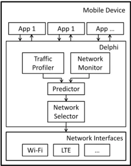
Mobile Device App 1 Delphi Wi‐Fi LTE … Traffic  Profiler Network Monitor Predictor Network  Selector App 1 App … Network Interfaces

Figure 1: Delphi design.

Systems and APIs to exploit multiple interfaces. The idea of using multiple networks for increased capacity and fault-tolerance has attracted significant attention from researchers over the past decade. Early work [6] shows the benefits of combining multiple networks and shows use cases where selecting the right network can reduce energy consumption, enhance network capacity, and manage mobility.

FatVAP [16] and MultiNet [10] improve throughput by allowing a single Wi-Fi card to connect to multiple APs. COMBINE [4] improves individual device throughput by leveraging the wireless wide area network of neighboring de-vices. Blue-Fi [5] is a system that uses Bluetooth and cellular tower information to predict whether Wi-Fi is available to reduce Wi-Fi duty cycle. Airdrop [2], a feature of Apple OS X, allows users to share files over both Wi-Fi and Bluetooth. However, it is designed explicitly for the purpose of file shar-ing (a long-runnshar-ing flow), while our system focuses on the more common case of both short and long flows on mobile devices today.

Contact Networking [8] provides localized network com-munication between devices with multiple networks and fo-cuses on designing mechanisms that enable lightweight neigh-bor discovery, name resolution, and routing. Intentional Net-working [14] provides APIs that allow apps to label their network flows. The labels include background or foreground to specify whether the flow is delay-tolerant, and large or small to specify the amount of data to be transmitted. In-tentional Networking uses a connection scout that probes net-work conditions periodically, an overhead Delphi can avoid by using passive measurement only. We consider these abstrac-tions orthogonal because Delphi’s network selection policy is agnostic to the API exposed by the system to applications. Delphi can be used as a decision-making module to select network interfaces within these systems.

3. O

Delphi uses three pieces of information to select the

net-work(s) to use for a data transfer:

1. App traffic profile: how much data does a transfer send or receive, for example, as part of a HTTP transaction. 2. Network conditions for the wireless interfaces, for

ex-ample, channel quality, current load in the network, end-to-end delay, etc. This information allows us to es-timate higher-layer network performance metrics, such as flow completion time, average burst throughput, etc. 3. The objective function to be optimized, such as the flow completion time, energy per byte, or monetary cost for the transfer.

Figure 1 shows the four components in Delphi, which is implemented as a software controller between the application and transport layers. The Traffic Profiler (Section 4) estimates transfer sizes, and the Network Monitor (Section 5) collects data needed for the Predictor to predict current network per-formance. The Predictor (Section 6) feeds the prediction to Network Selector (Section 7), which selects the network(s) to optimize the specified objective. Implementing this design requires no modification to applications (Section 8).

4. T

P

Recent study [11] analyzed 90,000 Android apps and found that 70,000 of them used HTTP or HTTPS, and that among the 70,000, 70% of them used HTTP and not HTTPS. Thus, we design the Traffic Profiler by first focusing on HTTP.

When a mobile user downloads a file using a HTTP GET, the HTTP GET response header usually contains a “Content-Length” field specifying the length of the response. Dur-ing uploads, the mobile device issues a HTTP POST whose “Content-Length” field specifies the transfer size. In both cases, the Content-Length field provides the relevant transfer size information to the Traffic Profiler readily.

Count Percentage

HTTP Transactions 59679 100%

Transactions with Content-Length 50865 85%

Predictable Transactions 50613 84%

Chunked-Encoding Transactions 3559 6%

Table 1: HTTP transaction data lengths for the Alexa top-500 sites. 84% of the transfer lengths are predictable by the Traffic Profiler.

However, the “Content-Length” field is not mandatory for HTTP headers; for instance, HTTP transactions often use chunked encoding when the length of data to be transmitted is dynamic. To determine how many HTTP transactions contain the “Content-Length” header, we use a record-and-replay tool, Mahimahi [23], to record the HTTP requests and responses when loading the homepage of the Alexa top-500 websites [3]. The results are listed in Table 1. When each site is loaded once, the total number of HTTP transactions are 59679. We note that 84% of the transactions are predictable by Traffic Profiler. Here, predictable means relative difference between the “Content-Length” value and the actual amount of data transmitted is less than 10%. Thus, using the

“Content-Length” field to predict the size of the data transfer works for most (84%) HTTP transactions. For HTTPS, the header is encrypted. To be able to look into the headers, we could set up a SSL proxy on the mobile device and make all traffic go through it [35].

Delphi also provides an API for the application to let the Traffic Profiler know how much data it is going to transfer. Compared with the Traffic Profiler monitoring data trans-missions on its own, this API allows the Traffic Profiler to unambiguously determine the amount of data the application is going to transfer. As shown in Section 6.2.1, providing accurate transfer length helps Delphi to make better network selection. This benefit can incentivize application developers to adopt the API for better performance, as while as better security guarantees (for applications using HTTPS).

The Traffic Profiler notifies the Predictor by sending it (TCP_CONNECTION_ID, data_length, direction) (direction means whether the device is downloading or up-loading data) when any of the following events occur:

1. an API call occurs from the app,

2. a request to initiate a new TCP connection is observed, 3. an HTTP request/response is observed.

The Traffic Profiler may not be able to tell how much data is going to be transmitted in Case 2, and sometimes in Case 3 (e.g., chunked encoding). In such cases, the Traf-fic Profiler will simply return a data_length of 3 KB. Once chunked encoding was observed, the profiler up-date predicted transfer size to be 100 KB. We chose these numbers because they are the median values of data transmis-sion length observed in Alexa top-500 sites. Section 6.2.1 analyzes how these default data length values affect network selection results.

5. N

M

The Network Monitor tracks a set of network-condition indicators for both Wi-Fi and LTE, and notifies the Predictor whenever an indicator value changes.

Category Wi-Fi Indicators LTE Indicators Passive Indica-tors RSSI, Link Speed,Wi-Fi AP Count Signal Strength, DBM, RSSNR, CQI,RSRP, RSRQ, Wi-Fi AP Count Active

Probing Max/Min/Mdev Ping RTT, DNS Lookup Time, UDPthroughput, UDP lossrate, UDP packet Inter-arrival-time mean/median/90 percentile

Table 2: Network Indicators monitored by Delphi. 5.1 Network Indicators

Table 2 lists the indicators used by Delphi. These indicators are categorized into 2 sub-groups: passive measurement and active probing. The passive measurements capture channel quality and contention for the last-hop wireless link, which is often the bottleneck along both the forward and reverse paths between the mobile device and the Internet. However, this last-hop information does not always reflect network condi-tions along the whole path. For example, for LTE networks,

the delay introduced by packet buffering at the cell tower side can be significant [15], but is not captured by last-hop passive measurements. Wi-Fi access in public areas such as shopping malls, airports, etc. may be subject to bandwidth limits introduced at the gateway to the Internet, and these are not captured by last hop measurements. To capture these non-last-hop, or end-to-end network performance factors, Delphi also runs active probes between the mobile device and an Internet server (see Section 8).

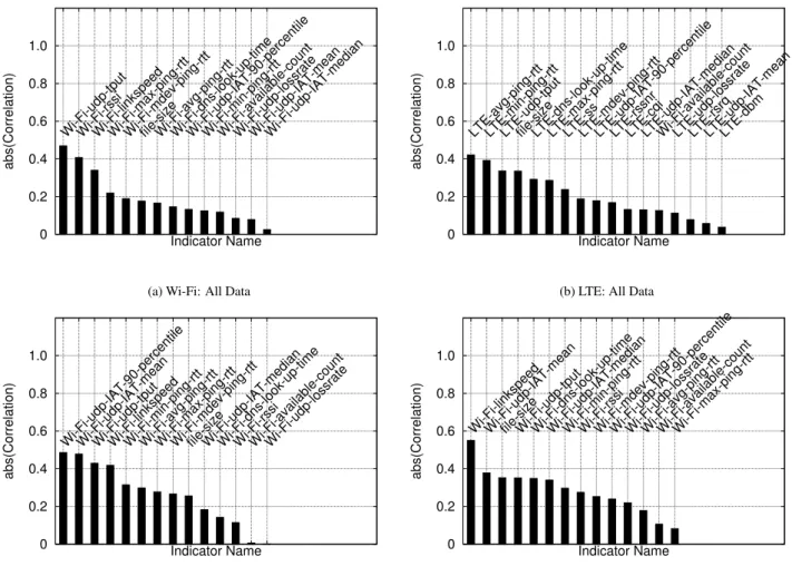
To quantify how each indicator affects TCP throughput, we analyze data collected from 22 locations. Those locations included shopping malls, Wi-Fi-covered downtown areas, and university campuses, where both Wi-Fi and LTE were available. At each location, the total measurement time is at least 1 hour. We compute the Pearson Correlation [37] between the throughput and each indicator. The correlation is a number between -1 and 1, inclusive. A value close to 1/-1 means strong positive/negative correlation. A value close to 0 means weak correlation.

Figure 2 shows the absolute value for correlation between throughput and each indicator. The bars in each sub-figure are sorted from strongest to weakest correlation. Figure 2a and 2b shows the correlation over the entire dataset. For both Wi-Fi and LTE, among the most correlated indicators, we see both active probing indicators (such as Wi-Fi UDP throughput and LTE Average Ping RTT) and passive indicators. Figure 2c and 2d show the correlation values calculated using data collected at only one location. Compared to Figure 2a, at each location, the order of the correlation strength changes. Similar results can be seen in LTE and MPTCP analysis. 5.2 Adaptive Probing

Probe Type DNS Query 10 Pings UDP

Data Transferred (Bytes) 271 1K 200K

Wi-Fi Median Delay (Sec) 0.64 9.02 0.65

Wi-Fi Energy (mJ) 331 4730 366

Cellular Median Delay (Sec) 0.63 9.01 0.58

Cellular Energy (mJ) 1378 19697 1613

Table 3: Overhead for one occurrence of active probing. The delay values are the median value across all measurement data collected at 22 locations. The energy values are measured in a indoor setting. The cellular energy values do not contain tail-energy [12].

As shown in Figure 2, actively probing the network can provide important information to estimate network perfor-mance. However, active probing can be expensive in terms of energy, bandwidth and delay. Table 3 summaries the over-head in terms of delay, amount of data transferred, and energy consumption.

To reduce the probing overhead, the Network Monitor probes the network adaptively, only if there is a significant change in the passive indicators. Otherwise, it will reuse active probing information collected previously. To further reduce probing overhead, Delphi adaptively probes only when the mobile device’s screen is on, which suggests that the

0 0.2 0.4 0.6 0.8 1.0

Wi-Fi-udp-tputWi-Fi-rssiWi-Fi-linkspeedWi-Fi-max-ping-rttWi-Fi-mdev-ping-rttfile-sizeWi-Fi-avg-ping-rttWi-Fi-dns-look-up-timeWi-Fi-udp-IAT-90-percentileWi-Fi-min-ping-rttWi-Fi-available-countWi-Fi-udp-lossrateWi-Fi-udp-IAT-meanWi-Fi-udp-IAT-median

abs(Correlation)

Indicator Name

(a) Wi-Fi: All Data

0 0.2 0.4 0.6 0.8 1.0

LTE-avg-ping-rttLTE-min-ping-rttLTE-udp-tputfile-sizeLTE-dns-look-up-timeLTE-max-ping-rttLTE-ssLTE-mdev-ping-rttLTE-udp-IAT-90-percentileLTE-rssnrLTE-cqiLTE-udp-IAT-medianWi-Fi-available-countLTE-udp-lossrateLTE-rsrqLTE-udp-IAT-meanLTE-dbm

abs(Correlation)

Indicator Name

(b) LTE: All Data

0 0.2 0.4 0.6 0.8 1.0

Wi-Fi-udp-IAT-90-percentileWi-Fi-udp-IAT-meanWi-Fi-udp-tputWi-Fi-linkspeedWi-Fi-min-ping-rttWi-Fi-avg-ping-rttWi-Fi-max-ping-rttWi-Fi-mdev-ping-rttfile-sizeWi-Fi-udp-IAT-medianWi-Fi-dns-look-up-timeWi-Fi-rssiWi-Fi-available-countWi-Fi-udp-lossrate

abs(Correlation) Indicator Name (c) Wi-Fi: Location 1 0 0.2 0.4 0.6 0.8 1.0

Wi-Fi-linkspeedWi-Fi-udp-IAT-meanfile-sizeWi-Fi-udp-tputWi-Fi-dns-look-up-timeWi-Fi-udp-IAT-medianWi-Fi-min-ping-rttWi-Fi-rssiWi-Fi-mdev-ping-rttWi-Fi-udp-IAT-90-percentileWi-Fi-udp-lossrateWi-Fi-avg-ping-rttWi-Fi-available-countWi-Fi-max-ping-rtt

abs(Correlation)

Indicator Name

(d) Wi-Fi: Location 2

Figure 2: Correlation between Wi-Fi/LTE single path TCP throughput and each indicators. user is currently interacting with the device, and is more

sensitive to network delays. There are, of course, times when background applications also need low delays (e.g., a cloud-based navigation app), but in the common case, delay is less of a concern in such situations. For background transmissions, Delphi will only probe the network when both conditions occur: 1) there is a large change in the passive measurements; and 2) there is a data transmission request.

Adaptive probing has two benefits:

1. It is energy-efficient compared with fixed-rate probing. 2. It is proactive compared with probing only on a

trans-mission request, which would delay the request. To evaluate adaptive probing, we simulate it using our collected data as follows. We take the first run’s passive and active measurement as input. Then, for the second run, we compare the passive measurement values with the first run. If the passive measurement difference d is less than a certain threshold Th, we keep the first run’s active probing values as our measured number, and use the second run’s active probing values as the ground truth to calculate an error e. If d is greater than Th, we do active probing again.

The definitions of d and e for a run r are: dr= m

∑

∑

Here, m is the total number of passive indicators. piis the

value of the passive indicator i. pi,maxand pi,minare the max

and min values for these indicators. n is the total number of active indicators. ˆaj,ris the active probing value for indicator

j and aj,ris the ground truth value, in run r.

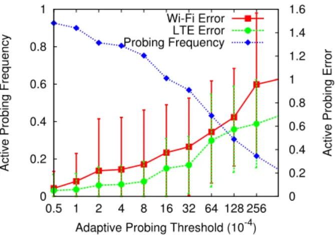
Figure 3 shows that as the probing threshold increases, fewer probes are triggered. Also, as the probing threshold increases, the error of reusing the previous active probing value increases. In Section 6, we will analyze the extent to which the choice of network is affected by this adaptive probing error.

0 0.2 0.4 0.6 0.8 1 0.5 1 2 4 8 16 32 64 128 256 0 0.2 0.4 0.6 0.8 1 1.2 1.4 1.6

Active Probing Frequency

Active Probing Error

Adaptive Probing Threshold (10-4) Wi-Fi Error

LTE Error Probing Frequency

Figure 3: As the adaptive probing threshold (x-axis) increases, the number of probing decreases and the probing error in-creases. Here the left y-axis shows the probing frequency, which is the average number of proving in every five minutes. Delphi’s Predictor takes the traffic profile and network sta-tus as input to estimate network performance. In this section, we focus on how it estimates TCP flow completion time, because flow completion time is used in all our objectives mentioned in Section 7. However, similar techniques can be used to estimate other metrics such as average throughput (for steaming applications) or average RTT (for interactive applications).

To predict TCP flow completion time, or related metrics such as the end-to-end throughput for Wi-Fi and LTE net-works, previous work either uses historical data from the same flow to predict current throughput [40], or outputs bi-nary results such as high/low throughput [9]. However, for Delphi, the prediction is more challenging: first, it needs to make its decision just before the connection transfers data and recent historical data may not always available. Second, it needs to return numerical values instead of binary results to be fed into the Selector.

We use a machine learning model, Regression Tree [26] to estimate TCP flow-completion time. This learning method matches well with our problem definition, as it takes multi-dimensional vectors as input, and produces a real-valued result. In our case, the multi-dimensional input includes data size and network condition indicators. Another advan-tage of using a regression tree is that by assigning different weight to different indicators when traversing through differ-ent branches, per-location differences (Figure 2) are captured naturally. Regression trees have been used to solve other network performance estimation problems [40] due to its low memory and computation overhead.

Delphi constructs the four regression trees to predict the flow completion time for single-path TCP over Wi-Fi or LTE, and for MPTCP using Wi-Fi or LTE for the primary subflow. We estimate the flow completion time of MPTCP using sep-arate trees, instead of deriving it from the flow completion

0 0.25 0.5 0.75 1.0 0 0.1 0.2 0.3 0.4 0.5 CDF Relative Error Tree SVR

(a) TCP over Wi-Fi

0 0.25 0.5 0.75 1.0 0 0.1 0.2 0.3 0.4 0.5 CDF Relative Error Tree SVR (b) TCP over LTE

Figure 4: Relative error when using regression tree and sup-port vector regression to learn flow-completion time. The line marked with “Tree” shows the relative error of regression tree model. The line with “SVR” shows the relative error of support vector regression model.

time estimated for single-path TCP, because previous mea-surement study [13] shows that throughputs of single-path TCP over two networks do not add up to the throughput of MPTCP. Besides, there are cases where MPTCP over both networks gives lower throughput than single-path TCP over a single network.

The prediction accuracy is affected by two factors: 1. the predictive power of the machine learning model, i.e.,

whether regression trees are a good model for predicting flow completion time, and

2. the measurement accuracy of the inputs to the machine-learning methods.

6.1 Regression Tree Prediction Accuracy

Here, we use our dataset collected from 22 locations to analyze Delphi’s prediction accuracy. To train the regression tree model, we randomly select 10% of the total samples from our dataset. We then use the remaining 90% as our testing data. As a comparison, we also trained support vector regression (SVR) models with radio basis kernel [29], which also take a multi-dimensional vector as input and outputs numerical results. The SVR models also consists of four separate models, each for one network configuration. To train each SVR model, we first sort all the indicators from the most-correlated to the least-most-correlated with the flow completion time. Here, we compute the correlation across all the data, not just the 10% in the training set, so that the sorting would not be biased by the training set. Then, we train the SVR model using the N most correlated features. As N increases, the testing errors first decrease (because the model improves in predictive power) and then increase (because the model overfits to the training set). For each SVR model, we choose the N that gives the smallest error. Thus, the resulting models are the best that can be achieved using the SVR method given the features that we measure.

We test both models using the same testing set. Figure 4 shows the CDF of relative error between the learned result and the ground truth when predicting Wi-Fi and LTE. MPTCP pre-dictions give similar results. Here, the regression-tree model predicts the flow completion time with smaller error than the

0 0.1 0.2 0.3 0.4 0.5 0.6 0.7 0.8 0.9 1 0 0.2 0.4 0.6 0.8 1 CDF Relative Error 5 KB 10 KB 100 KB 1 MB

Figure 5: Relative error when using an empirical flow size number (3 KB) to predict flow completion time. The legends are the actual flow sizes.

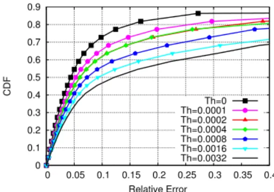
0 0.1 0.2 0.3 0.4 0.5 0.6 0.7 0.8 0.9 0 0.05 0.1 0.15 0.2 0.25 0.3 0.35 0.4 CDF Relative Error Th=0 Th=0.0001 Th=0.0002 Th=0.0004 Th=0.0008 Th=0.0016 Th=0.0032

Figure 6: Relative error when using adaptive probing to pre-dict flow completion time.

SVR model. Regression tree is more powerful because it is able to traverse through different paths in the tree when predicting different locations.

The median testing error ranges from 2% to 10% across the four regression tree models. Given that the training set only consists of 10% of the data, this shows the TCP flow completion time is predictable using regression trees. 6.2 Input Error Analysis

Section 6.1 shows the prediction error when the input fea-ture vectors are accurate. As described earlier, the Traffic Profiler sometimes needs to guess the transfer size, and the Network Monitor may reduce active probing frequency to reduce energy and traffic overhead. Thus, the input to the regression tree is not always perfect. In this section, we investigate what impact do these imperfections have. 6.2.1 Traffic Profiler Error

As mentioned in Section 4, when there is no “Content-Length” field specified in a burst of transmission, the Traffic Profiler returns an empirical number of 3 kbytes. Figure 5 shows the relative error using an inaccurate transfer size as a regression tree’s input (in Figure 5, we only show the results for TCP over LTE for clarity, but similar results hold for Wi-Fi and MPTCP). Here, we split the testing dataset into smaller

subsets, each subset contains measurement done for a certain transfer size. As the difference between the actual transfer size and 3 KB increases, the relative error increases. The prediction error is significantly higher than the previous 2%-10%. Fortunately, however, only less than 15% of transfers

are affected by this error, as noted in Section 4. 6.2.2 Network Monitor Error

Another source of error is adaptive probing. We run the regression tree testing over different Th values, which is an adaptive probing parameter. Figure 6 shows the CDF curves of relative errors for LTE. Here, as Th increases (i.e., probing less frequently), the prediction error increases. Wi-Fi and MPTCP predictions also gives similar results.

7. N

S

Delphi’s Selector uses network performance predictions, transfer lengths, and the specified objectives for application transfers to determine which network to use. The choice of network depends on three factors: throughput, energy efficiency, and monetary cost.

7.1 Objective Functions

Throughput, S: The Selector can estimate the average throughput of the current transfer using the transfer size f that is provided by the Traffic Profiler, and the flow completion time t that is provided by the Predictor. Using the subscript i to refer to the choice of the network (either Wi-Fi or LTE or MPTCP with a specified primary subflow), we have:

Si=_tf

i (3)

Energy per byte, Ei: Knowing the power level piof each

network choice i, together with the above tiand f , the energy

to transmit one byte is:

Ei= pi_f·ti (4)

The energy per byte is a metric that captures both battery consumption and transfer rate. A faster transfer over a net-work that has a higher power consumption may incur a lower energy per byte. As a result, minimizing energy per byte is not always the same as picking the network with lowest power consumption.

Monetary cost per byte, Mi: The “dollar” cost incurred

when transferring each byte of the transfer on network choice i.

By knowing Si, Eiand Mi, the Selector chooses the network

that maximizes the following objective function:

Oi= Si

α

Eiβ· Miγ (5)

This objective function prefers networks with high Si

val-ues, meaning in a given second, it wants the device to transfer

more bytes. It also prefers networks with low Eivalue,

mean-ing when consummean-ing one Joule of energy, it wants the device to transfer more bytes. Similarly, it prefers network with low

Mivalues, meaning when consuming one dollar, it wants the

device transfer more bytes.

The exponents α, β, γ ∈ [0,∞) determine the relative im-portance of throughput, energy efficiency, and monetary cost respectively. For example, if α = 1, β = 0 and γ = 0, then

Oi= Si, and the Selector will select the network with

high-est average throughput. This optimization is realistic if the device has an unlimited data plan and is connected to a AC power source. As another example, if α = 0, β = 1 and γ = 0,

then Oi= 1/Ei, and the Selector will select the network that

consumes the least amount of energy. This optimization is preferable when the device is about to run out of battery.

In our experiments, we set α, β, γ to different values to experiment with different scenarios. In a more realistic implementation, α, β and γ can be pre-defined by users, or decided by Delphi dynamically according to the phone’s current status. For example, β can increase as the battery level decreases. If the mobile device user has a limited monthly data plan for a cellular network, γ can increase as the amount of data plan consumed is approaching the budget, and fixed at a large number once the cellular usage exceeds the budget. Picking different values of α, β and γ makes the objective function expressive enough to handle a range of preferences. 7.2 Energy Model

Interface LTE Wi-Fi

Send Tput (mbps) 2.3 ∼ 4.4 7.4∼ 9.4 Send Power (mW) 2778± 56 536 ± 23 Recv Tput (mbps) 0.1∼1.5 7.3∼9.5 Recv Power (mW) 1674 ± 95 428 ± 58

Table 4: Power Level measurement for Wi-Fi and LTE.

An energy model is required to estimate Ei. We measured

the power level of both Wi-Fi and LTE by connecting the phone to a power monitor [18]. We measured the power level during both TCP uploads and downloads using Wi-Fi and LTE. We also measured the power level across different transmission rates for both Wi-Fi and LTE, by changing the underneath channel quality. To do so, for Wi-Fi, we change the distance between the phone and the access point. For LTE, we change the channel quality by moving into and out of buildings.

Table 4 shows the results. For each network, both while uploading and downloading data, the power level stays the same regardless of the data rate. Hence, we model the power

pi for each network using two constant numbers (one for

upload and one for download). However, for LTE, there is an additional “tail energy” [12] component that is consumed after a transfer finishes, which we treat as a constant number. As a result, when estimating the energy consumed for LTE, Delphi adds this tail energy to the total energy consumed. 7.3 Selector Performance

To quantify the Selector’s performance, we run simulations using data that we collected from 22 locations. We wrote a custom-built simulator that operates on this data set as

0 0.5 1 1.5 2 2.5 3 3.5 4 0 1 2 3 4 5 6 7 Th roug hpu t (MB its/S ec)

Energy Efficiency (MBits/J)

Max(S/E) Max(S)

Wi-Fi LTE

MPTCP(Wi-Fi)

MPTCP(LTE) _{Oracle Frontier}

Figure 7: Median megabits per Joule and throughput values for different schemes. The black line shows a frontier of the best that can be achieved when setting α = 1, γ = 0 and changing β from 0 to 5.

Objective Max(S) Max(S/E) Wi-Fi

Throughput (Mbits/Sec) 3.0 2.6 1.4

Energy Efficiency (Mbits/J) 2.8 4.9 5.2

Table 5: Median values for Max(S), Max(S/E) and Wi-Fi as shown in Figure 7.

described below. The dataset collected earlier maps a feature vector (made of up all the features listed in Table 2) to a tcpdump trace captured when running standard TCP on Wi-Fi and LTE and a tcpdump trace for MPTCP in striped mode using Wi-Fi as the primary subflow and using LTE as the primary subflow.

When evaluating any scheme, we assume all the features required by Delphi are available at the beginning of each run. We run Delphi’s selection algorithms described earlier using the features collected at the beginning of the run along with flow size as input. We then pick the network interface that maximizes the objective function described above and look at the previously collected tcpdump trace to determine the duration from the beginning of the trace until a transfer size worth of bytes are transferred. We repeat the same procedure, without any prediction, for the other policies for every run at each location.

In these simulations, we set γ = 0, meaning we do not consider monetary cost. Figure 7 shows the simulation results. The x-axis of the figure shows the number of bits that can be transmitted when consuming 1 Joule. The y-axis shows the throughput. We first draw a frontier line by changing β from 0 to 5. When computing the frontier, we also use the ground-truth value of each flow’s completion time, so that the frontier represents the best that can be achieved if we have a perfect predictor. We call this line “Oracle Frontier”.

In Figure 7, Wi-Fi, LTE, MPTCP(Wi-Fi) and MPTCP(LTE) are four fixed schemes, where the same network is used across all locations. Here Wi-Fi and LTE refer to transmitting data using single path TCP over Wi-Fi or LTE. MPTCP(Wi-Fi) and MPTCP(LTE) refer to transmitting data over MPTCP,

0 0.25 0.5 0.75 1.0

OracleDelphi OracleDelphi OracleDelphi

Selected Ratio LTE Wi-Fi MPTCP(LTE) MPTCP(Wi-Fi) Max(1/E) Max(S/E) Max(S)

Figure 8: Percentage of each network(s) is selected when using different objective functions.

0 20 40 60 80 100 Max(S/E) Max(S) Success Rate (%) Active Adaptive 3 KB

Figure 9: Success Rate for different schemes. while use Wi-Fi or LTE for primary subflow. “Max(S)” and “Max(S/E)” are two schemes run by the Selector. In Figure 7, the two Delphi schemes, “Max(S)” and “Max(S/E)”, fall close to the frontier line. In “Max(S)”, the Selector set β = 0, meaning it is simply trying to maximize throughput. In “Max(S/E)”, β = 1, meaning it tries to select networks with high throughput but without consuming too much energy. We can see that “Max(S)” and “Max(S/E)” are much closer to the Oracle Frontier line than any other schemes.

Table 5 lists the x and y-axis values for “Max(S)” and “Max(S/E)”, together with the median value for the fixed scheme that always uses Wi-Fi for comparison. Here, “Max(S)” gives the highest median throughput of 3.0 Mbits/sec, which is a 2.1x gain over Wi-Fi’s 1.4 Mbits/sec. “Max(S/E)” tries to achieve high throughput with high energy efficiency. Its median energy efficiency is 4.9 Mbits/J, 6% worse than al-ways using Wi-Fi, but it achieves a median throughput of 2.6 Mbits/sec, a 1.9x gain over Wi-Fi.

We now take a closer look at each scheme: when an ob-jective function is defined, how many times is each available choice selected? Figure 8 shows the percentage of time that each network choice is selected when trying to optimize differ-ent objectives. First, we can see that Delphi makes very simi-lar decisions compared with an omniscient oracle. However, for each specific objective function, Delphi chooses different networks. For example, when maximizing throughput,

Del-phi selects LTE more often than Wi-Fi or any other MPTCP-based scheme because LTE provides the highest throughput in most cases in our dataset. For “Max(S/E)” (maximizing throughput over energy), or for “Max(1/E)” (minimizing en-ergy consumption), Delphi tends to choose Wi-Fi much more often, since Wi-Fi is generally more energy-efficient. How-ever, both the oracle and Delphi still select other network(s) because there are cases where Wi-Fi gives really low through-put, lengthening the transfer and consuming significant energy in the process.

To understand these errors in more detail, we compare the decision made by the oracle and by Delphi. We say that Delphi makes a successful decision if it selects the same net-work(s) as the oracle. Figure 9 shows the ratio of successful decisions affected by different error sources. Here, “Active” refers to using active probing information for flow-completion time prediction. “Adaptive” refers to our adaptive probing technique described earlier. “3 KB” refers to the using active probing, where the traffic profiler outputs “3 KB” in 16% of the total outputs. We select 16% because we found that in 16% of the total network transactions’ data size is not predictable (Table 1 in Section 4).

We can see that “Active” gives highest success ratio (93% for Max(S/E) and 85% for Max(S)). As we add error to the network measurement input, i.e., “Adaptive”, the success ratio is lower (90% and 81% respectively). Finally, inaccurate transfer size information gives us the lowest success rate (86% and 78% respectively). These results show that we can achieve high success rates by adding active probing overhead. If the overhead is a concern, removing active probing can still give reasonable results. However, being able to predict the size of the burst of traffic is more important.

7.4 System Generalization

Model Type Obj. Throughput

(Mbits/Sec) Energyficiency Ef-(Mbits/J)

SVR Max(S) 2.3 1.6

Reg. Tree Max(S) 2.1 2.0

Wi-Fi Only - 1.4 5.6

LTE Only - 1.7 1.5

SVR Max(S/E) 1.4 5.6

Reg. Tree Max(S/E) 1.9 2.7

Table 6: Median values for throughput and energy efficiency when testing different model at new locations.

In our above analysis, our both training and testing datasets are generated from the 22 locations we measured. These results show the improvement when we have prior knowledge of the network condition of each location. In this section, we show the result in a more challenging condition: we test Delphi’s performance when there is no prior knowledge. This corresponds to the real use case where a smartphone user enters a new location that he/she has never been to.

We train Delphi using data collected from 21 out of the 22 locations, and test it on the last location. We repeat this

process 22 times by using each location to be the testing set. Table 6 shows that when maximizing throughput, Delphi achieves up to 1.6x (when using SVR model) improvement over Wi-Fi. When maximizing throughput over energy con-sumption, Delphi behaves as good as Wi-Fi and better than using LTE only. These results show that: 1) when there is no prior knowledge, the improvement decreases; 2) SVR model achieve higher improvement than Regression Tree. This is because Regression Tree is powerful when characterizes data in training set, which means it tend to overfit and being less powerful when predicting new data. Thus, Delphi can use SVR model to make decisions when entering new locations, or crowd-sourcing measurement techniques [32] can be used to feed the smartphone with prior knowledge of new loca-tions, to further improve performance. The details of model generalizing is part of our future work.

8. I

We implement Delphi on a laptop (2.4GHz Due Core with 4GB RAM, comparable to a smartphone) running MPTCP enabled (Ubuntu Linux 13.10 with Kernel version 3.11.0, with the MPTCP Kernel implementation version v0.88 [22]). We tethered two smartphones to the laptop, one in “airplane” mode with Wi-Fi enabled, and the other with Wi-Fi disabled but connected to the Verizon LTE network. The reason we im-plemented Delphi on laptop instead of Android phones is that we want to utilize already existed machine learning libraries. Importing the machine learning algorithms into Android plat-form will be our future work. We also enabled MPTCP on Galaxy Nexus running Android 4.1 [19] to validate that all the following functionality is feasible on smartphones. All the measurement data used for simulation in the previous settings are also collected under the same setting.

The current implementation of Delphi is a user-level appli-cation implemented in Python. One thread of Delphi serves as the Network Monitor; it continuously polls passive indicator values from both phones over the USB interface very 500 milliseconds.

Switch Type Send Delay (ms) Recv Delay (ms)

LTE switch on 494± 1 507 ± 13

Wi-Fi switch on 495 ± 2 782 ± 47

Table 7: Switching delay, averaged across ten measure-ments. The switching delay is defined as the time between a iptable rule changing command is issued and a packet transfer occurred on the newly brought up interface. The send delay is the delay for the first out-going packet showing up, and the receive delay is for the first ACK packet coming from the server.

The other thread serves as the Traffic Profiler, Predictor and Selector. It runs tcpdump to monitor packet transmis-sions in real time. Once it sees that a network transfer has been initiated, it looks for a HTTP request or response header and reads the “Content-Length” information from the header. It then calls the prediction function to predict the transfer

completion time, and then calls the Selector function to se-lect the a single network by changing iptable rules [21]. These procedure of turning an interface off allows MPTCP to migrate to the new connection because it supports break-before-make semantics. When the network is idle, this thread also reads the passive indicator values periodically (every 5 seconds), and uses a default value of “3KB” as transfer length when calling the Predictor and Selector function, so that the network can be pre-selected before a new TCP connection starts. When a connection is actively transmitting, Delphi also periodically (every 1 second) reads the passive indicator values, so that it can detect significant network environment changes, in case the mobile device is moving. This allows Delphi to dynamically select networks during long-running transfers. Once the Selector decide a interface switching is re-quired, it achieves the switch by changing iptable entries for that specific TCP connection. Table 7 shows the interface switching delay measured in a indoor setting. Each number is an average across ten measurements. The switching delay is defined as the time between a iptable rule changing com-mand is issued and a packet transfer occurred on the newly brought up interface. In our currently implementation, the out-going delay is 500 ms. During this 500 ms, the transfer does not pause, but continues on the pre-selected network. Noticed that not all connections will experience this delay because Delphi can pre-select the network configurations as it observes a network condition change. This switch delay will only happen when 1) network condition changes during a transfer 2) the network selection result based on the actual transfer size is different from the result based on the default “3KB” value. In our experiments (Section 9.2), 18% of HTTP

transactions needs a network switch during data transfer. We configured the laptop to pass all its HTTP traffic through an MPTCP-enabled proxy server. Because current app servers do not always support MPTCP, the proxy server allows our client to run apps over MPTCP, while talking to the apps’ orig-inal server. Also, since MPTCP is enabled on both the client and the proxy server, we can migrate connections from Wi-Fi to LTE easily using ip link set dev [interface] multipath on/off, without breaking them.

9. E

In previous sections, we analyze the performance of each module using a trace-driven approach. This serves as micro-benchmark evaluation of Delphi. In this section, we focus on macro-benchmark evaluation done by emulation and real-world experiments.

9.1 Delphi over Emulated Networks

To understand Delphi’s performance under real applica-tion workloads, we use Mahimahi [23], a record-and-replay tool that can record and replay client-server interactions over HTTP. In our experiment, we record client-server interac-tions when the client runs two applicainterac-tions: Web brows-ing and video streambrows-ing. Durbrows-ing replay, Mahimahi replays the recorded interactions on top of an emulated network.

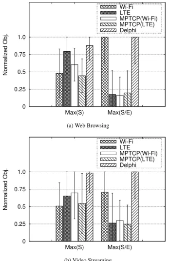
0 0.25 0.5 0.75 1.0 Max(S) Max(S/E) Normalized Obj. Wi-Fi LTE MPTCP(Wi-Fi) MPTCP(LTE) Delphi

(a) Web Browsing

0 0.25 0.5 0.75 1.0 Max(S) Max(S/E) Normalized Obj. Wi-Fi LTE MPTCP(Wi-Fi) MPTCP(LTE) Delphi (b) Video Streaming

Figure 10: Objective function value normalized by oracle. The histogram shows the median value, the error bar shows one standard deviation.

Mahimahi can emulate network delays and variable-rate links using packet-delivery traces. In our experiment, we used the tcpdump traces captured during our measurement at 22 loca-tions as packet-delivery traces for network emulation. During the tcpdump measurements, we also measured passive indi-cator values, which are fed into Delphi during our emulation as inputs to the Network Monitor. This emulation setup en-able us to compare different network selection schemes when running exactly the same application traffic, and under the same network conditions.

We use Delphi to optimize two different objective func-tions: 1) Max(S): maximizing average throughput, i.e. mini-mizing transfer completion time. 2) Max(S/E): maximini-mizing average throughput over energy per byte. In each experiment, we record the actual value of S and S/E achieved by Delphi and by using different fixed choices. After running Delphi and the fixed network(s) schemes at one location, we can determine which network choices gives the highest value of S and S/E. We call this highest value the optimal ground truth.

0 0.5 1 1.5 2 2.5 3

Loc-1 Loc-2 Loc-3 Loc-4 Loc-5

Normalized Tput

Location ID Wi-Fi

LTE Delphi

(a) Break down by locations

0 0.5 1 1.5 2 2.5 3 3.5 4 4.5 1KB 3KB 10KB 100KB 1MB Normalized Tput Transfer Sizes Wi-Fi LTE Delphi

(b) Break down by transfer sizes

Figure 11: Objective function value normalized by oracle. The histogram shows the median value, the error bar shows one standard deviation.

We use the optimal ground truth to normalize the predictions of all schemes that we consider.

Figure 10 shows the median normalized value for each scheme across all locations. Figure 10a shows the results for Web browsing. For Max(S), Delphi gives the highest through-put over all the other fixed schemes. When compared with Wi-Fi, which is the default network selection on most mobile devices, our throughput improvement is 83%, which corre-sponds to a 46% reduction in transfer time. For Max(S/E), Delphi improves the median normalized throughput over en-ergy per byte by 0% (over Wi-Fi, since Wi-Fi tends to be much more energy efficient than other schemes) to 6x (over MPTCP(Wi-Fi)). In Figure 10b, for video-streaming appli-cations, for Max(S), Delphi improves the throughput by 93% over Wi-Fi, corresponding to a 49% reduction in transfer time. For Max(S/E), Delphi’s improvement ranges from 41% (over Wi-Fi) to 3.9x (over MPTCP(LTE)).

9.2 Experiments

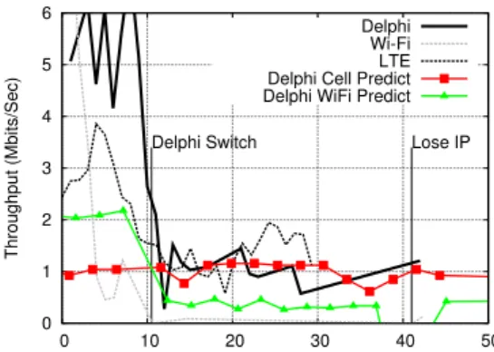
0 1 2 3 4 5 6 0 10 20 30 40 50 Throughput (Mbits/Sec) Lose IP Delphi Switch Delphi Wi-Fi LTE Delphi Cell Predict Delphi WiFi Predict

Figure 12: When the mobile device is moving away from an access point, Delphi predicts that Wi-Fi can be worse than LTE, then it switches to LTE at time 10.5 seconds. MPTCP handover mode switches to LTE when it sees Wi-Fi loses IP, which happens at time 41 seconds.

first train Delphi’s predictor using data we collected at the 22 locations. The model training was done using a desktop (Intel Xeon(R) CPU, 3.30GHz Quad Core, 16 GB RAM). The total training process takes 5 minutes. Then among the 22 locations, we visited 5 close to our campus. On our Delphi enabled laptop, we ran wget to download files with various sizes (1 KB, 3 KB, 10 KB, 100 KB and 1000 KB) from a remote server. For comparison, we also ran the same wget with only Wi-Fi or LTE enabled before or after we run Delphi. We randomized the sequence of configurations (file sizes, network measured). For each configuration, we ran five times.

Figure 11 shows the average improvement of Delphi over Wi-Fi and LTE, when Delphi’s objective is set to maximizing throughput. Due to high variation of the actual throughput across different configuration, here we show the throughput normalized by Wi-Fi’s throughput. Figure 11a shows Delphi’s performance at each location. We can see that Delphi does not perform perfectly well. At Location 3, the LTE has a higher average throughput than Wi-Fi, but Delphi still selects Wi-Fi. However, at other locations, Delphi performs better than always using Wi-Fi or LTE. At Location 2, 4 and 5, Delphi performs better than both Wi-Fi and LTE, because it uses MPTCP running over both networks. In Figure 11b, we can see that Delphi achieves improvement for small (1KB, 3 KB and 10 KB) and large (100 KB) transfers. A deeper investigation reveals that the middle sized (1 MB) transfers are affected by the switching delay the most: most of the transfers go through the sub-optimal network(s). However, for large transfers, although Delphi transfers on sub-optimal network(s) for some time, most of the transfer happens on the optimal network. Thus, Delphi performs well for large transfers. In summary, Delphi increases average throughput by between 1.25x and 4x compared with Android’s default policy which always use Wi-Fi when it is available.

9.3 Handling User Mobility

Another benefit of using Delphi is that by continuously monitoring the network conditions using the Network Moni-tor, Delphi can tell whether the network performance is get-ting worse, and trigger handover proactively. This is best demonstrated when the mobile device is moving. In this ex-periment, we keep Delphi running on the laptop while moving it from inside a building to outside a building. The tethered Wi-Fi phone was initially connected to the Wi-Fi AP inside the building. As we walk outside the building, the Wi-Fi signal keeps decreasing until the phone cannot associate with the AP. We run wget on the laptop to download a large file from our proxy server. (In this experiment, we configured Delphi to Max(S), and only select between Wi-Fi and LTE, not the MPTCP choices, to study the handover behavior). In our experiment, We first run wget without running Delphi, and with only one interface at a time, to measure the through-put of Wi-Fi and LTE as the laptop moves, shown as “Wi-Fi” and “LTE” in Figure 12. Then we run Delphi, while moving the laptop along the same path. In Figure 12, we can see that at time 10.5, Delphi predicted that Wi-Fi is worse than LTE, and consequently triggered a switch and the throughput drops but soon recovers to LTE’s throughput. In Figure 12, we also marked the time when the Wi-Fi phone loses its IP address; this is when a handover will happen according to Multi-Path TCP Handover-Mode proposed in [27]. However, we can see that in this case, Wi-Fi throughput has already dropped to zero before it loses IP address. Compared with this scheme, Delphi triggers LTE/Wi-Fi handover earlier, so that the application sees constantly high throughput.

10. C

F

W

We have presented Delphi, a mobile software controller to help applications select the best network among multiple choices for their data transfers. Delphi’s selection schemes are able to handle trade-offs between high throughput and energy efficiency. Thus it outperforms static schemes such as using Wi-Fi by default (the policy on Android today), or using LTE by default, or always using both, since neither Wi-Fi nor LTE is unequivocally better than the other, in terms of average throughput, and using both networks consumes an excessive amount of energy.

Applications could care about other metrics such as av-erage per-packet delay, and tail per-packet delay, or more app-centric metrics such as page-load time for web pages or minimizing the risk of a stall for streaming video. We view Delphi as a first step in answering these more involved questions. One direction of our future work is to provide ex-pressive APIs for applications to express their specific needs to Delphi.

In this paper, we use machine learning as a tool to make decisions where a static policy does not suffice. Another di-rection that we plan to explore is to further enhance Delphi’s learning capability by using online learning or crowd-sourced learning mechanisms. This would allow mobile devices to make better network selection decisions when they enter lo-cations for the first time.

R

[1] Y. Agarwal, T. Pering, R. Want, and R. Gupta. SwitchR: Reducing System Power Consumption in a Multi-Client, Multi-Radio Environment. In Wearable Computers, 2008.

[2] ios: Using airdrop. http://support.apple.com/ kb/HT5887.

[3] Top Sites in United States. http://

www.alexa.com/topsites/countries/US. [4] G. Ananthanarayanan, V. N. Padmanabhan, L.

Ravin-dranath, and C. A. Thekkath. Combine: Leveraging the Power of Wireless Peers through Collaborative Down-loading. In MobiSys, 2007.

[5] G. Ananthanarayanan and I. Stoica. Blue-Fi: Enhancing Wi-Fi Performance using Bluetooth Signals. In Proc. MobiSys, 2009.

[6] P. Bahl, A. Adya, J. Padhye, and A. Walman. Recon-sidering Wireless Systems with Multiple Radios. SIG-COMM CCR, 2004.

[7] F. Bari and V. Leung. Automated Network Selection in a Heterogeneous Wireless Network Environment. Net-work, IEEE, 21(1):34–40, Jan 2007.

[8] C. Carter, R. Kravets, and J. Tourrilhes. Contact Net-working: a Localized Mobility System. In MobiSys, 2003.

[9] A. Chakraborty, V. Navda, V. N. Padmanabhan, and R. Ramjee. Coordinating Cellular Background Transfers Using LoadSense. In MobiCom, 2013.

[10] R. Chandra and P. Bahl. MultiNet: Connecting to Mul-tiple IEEE 802.11 Networks Using a Single Wireless Card. In INFOCOM, 2004.

[11] S. Dai, A. Tongaonkar, X. Wang, A. Nucci, and D. Song. Networkprofiler: Towards Automatic Fingerprinting of Android Apps. In INFOCOM, 2013.

[12] S. Deng and H. Balakrishnan. Traffic-Aware Techniques to Reduce 3G/LTE Wireless Energy Consumption. In CoNEXT, 2012.

[13] S. Deng, R. Netravali, A. Sivaraman, and H. Balakrish-nan. WiFi, LTE, or Both? Measuring Multi-Homed Wireless Internet Performance. In IMC, 2014.

[14] B. D. Higgins, A. Reda, T. Alperovich, J. Flinn, T. J. Giuli, B. Noble, and D. Watson. Intentional Networking: Opportunistic Exploitation of Mobile Network Diversity. In MobiCom, 2010.

[15] H. Jiang, Z. Liu, Y. Wang, K. Lee, and I. Rhee. Under-standing Bufferbloat in Cellular Networks. In CellNet, 2012.

[16] S. Kandula, K. C.-J. Lin, T. Badirkhanli, and D. Katabi. FatVAP: Aggregating AP Backhaul Capacity to Maxi-mize Throughput. In NSDI, volume 8, 2008.

[17] R. Mahindra, H. Viswanathan, K. Sundaresan, M. Y. Arslan, and S. Rangarajan. A Practical Traffic Manage-ment System for Integrated LTE-WiFi Networks. In MobiCom, 2014.

[18] Monsoon Power Monitor. http:

//www.msoon.com/LabEquipment/ PowerMonitor/.

[19] MPTCP for Android.

http://multipath-tcp.org/pmwiki.php/Users/Android.

[20] Apple iOS 7 surprises as first with

new multipath TCP connections.

http://www.networkworld.com/news/2013/091913-ios7-multipath-273995.html. [21] Configure MPTCP Routing. http:// multipath-tcp.org/pmwiki.php/Users/ ConfigureRouting. [22] MPTCP v0.88 Release. http://multipath-tcp.org/pmwiki.php?n=Main.Release88. [23] R. Netravali, A. Sivaraman, K. Winstein, S. Das,

A. Goyal, and H. Balakrishnan. Mahimahi: A

Lightweight Toolkit for Reproducible Web Measure-ment (Demo). In SIGCOMM, 2014.

[24] S. Nirjon, A. Nicoara, C.-H. Hsu, J. Singh, and J. Stankovic. Multinets: Policy oriented real-time switching of wireless interfaces on mobile devices. In RTAS, 2012.

[25] D. Niyato and E. Hossain. Dynamics of Network Selec-tion in Heterogeneous Wireless Networks: An Evolu-tionary Game Approach. IEEE Transactions on Vehicu-lar Technology,, 58(4):2008–2017, May 2009.

[26] L. Olshen and C. J. Stone. Classification and Regression Trees. Wadsworth International Group, 1984.

[27] C. Paasch, G. Detal, F. Duchene, C. Raiciu, and O. Bonaventure. Exploring Mobile/WiFi Handover with Multipath TCP. In CellNet, 2012.

[28] A. Parekh and R. Gallager. A generalized processor sharing approach to flow control in integrated services networks: the single-node case. Networking, IEEE/ACM Transactions on, 1(3):344–357, Jun 1993.

[29] F. Pedregosa, G. Varoquaux, A. Gramfort, V. Michel, B. Thirion, O. Grisel, M. Blondel, P. Prettenhofer, R. Weiss, V. Dubourg, J. Vanderplas, A. Passos, D. Cour-napeau, M. Brucher, M. Perrot, and E. Duchesnay. Scikit-learn: Machine learning in Python. Journal of Machine Learning Research, 2011.

[30] T. Pering, Y. Agarwal, R. Gupta, and R. Want. Coolspots: Reducing the Power Consumption of Wire-less Mobile Devices with Multiple Radio Interfaces. In MobiSys, 2006.

[31] C. E. Perkins. Mobile IP. Communications Magazine, IEEE, 1997.

[32] S. Rosen, S.-J. Lee, J. Lee, P. Congdon, Z. Morley Mao, and K. Burden. MCNet: Crowdsourcing Wireless Per-formance Measurements through the Eyes of Mobile Devices. Communications Magazine, IEEE, 2014. [33] A. C. Snoeren and H. Balakrishnan. An End-to-end

Approach to Host Mobility. In MobiCom, 2000. [34] Q. Song and A. Jamalipour. Network Selection in

an Integrated Wireless LAN and UMTS Environment Using Mathematical Modeling and Computing Tech-niques. IEEE Wireless Communications, 12(3):42–48,

June 2005.

[35] SSL Proxy: Man-in-the-middle. http:

//crypto.stanford.edu/ssl-mitm/.

[36] Cisco visual networking index: Global mobile

data traffic forecast update, 2014-2019. http:

//www.cisco.com/c/en/us/solutions/ collateral/service-provider/visual-networking-index-vni/white_paper_ c11-520862.html.

[37] WiFi direct description. http://

en.wikipedia.org/wiki/Pearson_product-moment_correlation_coefficient.

[38] K. Winstein and H. Balakrishnan. Mosh: An interactive remote shell for mobile clients. In USENIX ATC, 2012. [39] D. Wischik, C. Raiciu, A. Greenhalgh, and M. Handley. Design, Implementation and Evaluation of Congestion

Control for Multipath TCP. In NSDI, 2011.

[40] Q. Xu, S. Mehrotra, Z. Mao, and J. Li. PROTEUS: Net-work Performance Forecast for Real-Time, Interactive Mobile Applications. In MobiSys, 2013.

[41] K.-K. Yap, T.-Y. Huang, Y. Yiakoumis, S. Chinchali, N. McKeown, and S. Katti. Scheduling Packets over Multiple Interfaces While Respecting User Preferences. In CoNEXT, 2013.

[42] K.-K. Yap, N. McKeown, and S. Katti. Multi-server Generalized Processor Sharing. In ITC, 2012.

[43] Google’s next bid to lower mobile data costs: Zero

rating. https://www.theinformation.com/

Google-s-Next-Bid-to-Lower-Mobile-Data-Costs-Zero-Rating.

[44] X. Zhao, C. Castelluccia, and M. Baker. Flexible Net-work Support for Mobility. In MobiCom, 1998.