Technology researchers and makes it freely available over the web where possible.
This is an author-deposited version published in: https://sam.ensam.eu
Handle ID: .http://hdl.handle.net/10985/6595
To cite this version :
Etienne PRULIERE, Amine AMMAR, Nadia EL KISSI, Francisco CHINESTA - Recirculating Flows Involving Short Fiber Suspensions: Numerical Difficulties and Efficient Advanced Micro-Macro Solvers - 2009
Any correspondence concerning this service should be sent to the repository Administrator : [email protected]
Recirculating flows involving short fiber
suspen-sions: numerical difficulties and efficient advanced
micro-macro solvers
Etienne Pruliere, Amine Ammar, Nadia El Kissi Laboratoire de Rh´eologie, UMR 5520 INPG-UJF-CNRS
1301 rue de la piscine, BP 53 Domaine universitaire, 38041 Grenoble Cedex 9, France E-mail: [email protected]
Francisco Chinesta
LMSP, UMR 8106 CNRS-ENSAM
151 Boulevard de l’Hpital, F-75013 Paris, France E-mail: [email protected]
Summary
Numerical modelling of non-Newtonian flows usually involves the coupling between equations of motion characterized by an elliptic character, and the fluid constitutive equation, which defines an advection problem linked to the fluid history. There are different numerical techniques to treat the hyperbolic advection equations. In non-recirculating flows, Eulerian discretizations can give a convergent solution within a short computing time. However, the existence of steady recirculating flow areas induces additional difficulties. Actually, in these flows neither boundary conditions nor initial conditions are known. In this paper we compares different advanced strategies (some of them recently proposed and extended here for addressing complex flows) when they are applied to the solution of the kinetic theory description of a short fiber suspension fluid flows.
1 Introduction
1.1 Recirculating flows of complex fluids
Understanding recirculating flows of complex fluids is of importance in many areas of poly-mer processing such as extrusion, injection or mixing. However, in such complex flows it is difficult to measure the detailed kinematics and stresses that develop during flow. It is thus necessary to predict them, by making good measurements of basic fluid properties and using them in the appropriate constitutive equations. This means taking into account the specific properties of complex fluids. Indeed, viscosity and shear thinning, elasticity and normal stresses, elongation and strain hardening as well as relaxation phenomena induce several unusual phenomena, and recirculating flows are one of them.
They have been observed in many flow configurations. In the case of Newtonian and inelastic fluids, their occurrence and evolution are mainly related to the inertial properties of the flow. Thus, the Rayleigh-Taylor instability occurs during flow between two coaxial cylinders [43], the external one being fixed while the internal one rotates. Due to centrifugal forces, the fluid is pushed from the inner cylinder towards the external one. Beyond a certain threshold, these forces cause recirculating flows in the form of rollers developing in the gap between the two cylinders. This is the well known inertial instability of Rayleigh-Taylor. Notice that the term instability in this case indicates that a secondary effect is superimposed on the main flow in controlling the kinematics. In fact, the recirculating areas are stable in
c
time and space. For a number of years now, many authors have studied the Rayleigh-Taylor inertial instability. Theoretical studies have analyzed the role of elasticity and showed that this property could stabilize flow, delaying, if not eliminating, the occurrence of the inertial instability [33].
It is also possible to observe recirculating flows independently of inertia. In the case of complex fluids for example, they result from properties such as viscosity, but also elastic-ity, elongation or relaxation phenomena. Such recirculating areas have been observed for example in flows through non-circular capillaries, typically of square or ellipsoidal section [34] [45] [23] [21]. They have also been observed when complex fluids flow through abrupt or shaped contractions, the fluid being pushed from a large-diameter reservoir, through a contraction and then into a capillary of smaller diameter. The high ratio between the capillary and reservoir diameters is defined as the contraction ratio. This flow configuration was the subject of thorough numerical as well as experimental studies. The reasons for this are numerous: From an academic point of view, this type of flow is of interest as an appro-priate test problem. They also allow the elongational properties of complex fluids, which are generally difficult to measure, to be evaluated [19] [10]. From an industrial point of view, contraction flows are of great importance in modelling polymer processing involving many contraction and expansion sections, such as extrusion. The occurrence, evolution, and geometrical characteristics of the recirculating areas developing upstream of the con-traction have a great impact in controlling the end-use properties of the material. Indeed, the recirculating fluid undergoes a thermo-mechanical history which is different from that of the flowing fluid. This can induce heterogeneities in the final properties of the material, thus affecting its mechanical characteristics and degradation properties. It is thus essential to understand and control the origin and development of such recirculating flows, the aim being to predict and optimize the kinematics with a view to eliminating secondary flows and regions of high stress.
If Newtonian or shear-thinning inelastic fluids are considered, it has been shown exper-imentally and by numerical simulation [24] [8] [28] [11] that inertia is responsible for the appearance of a recirculating area localized in the corner of the contraction.
The scenario is quite different when viscoelastic fluids are considered. The occurrence, evolution and shape of the recirculating zone are controlled completely by the viscoelastic properties. At low flow rates, the fluid behaves as a Newtonian fluid, with small vortices developing due to inertia. As the flow rate increases, the shape and size of the recirculating area are completely different from what is observed with Newtonian liquids. Two main phe-nomena are usually observed and are a good demonstration of viscoelastic behavior vortex enhancement the occurrence of a second recirculating zone, developing at the entrance of the contraction, called the lip vortex. Compared to Newtonian behavior where only small recirculating areas are observed, the two vortex areas coexist at low flow rates. As flow rates are increased, the lip vortex grows significantly, and progressively invades the corner vortex, leading to a single recirculating area in the upstream flow. The height of this re-circulating area may reach several reservoir diameters, thus invading a large proportion of the upstream flow. Thorough quantitative experimental studies, relating basic rheological measurements to the occurrence and evolution of the recirculating area patterns [20] [37], suggested that elasticity is responsible for vortex enhancement. Represented in terms of a Weissenberg number, this was used successfully to explain the variation in vortex size and in particular to correlate the growth of the recirculating area.
This situation is also encountered when flows involving short fiber suspensions are ad-dressed. In this case the size of the vortex appearing in abrupt contractions depends on the suspension concentration and can be accounted without introducing inertia effects [29].
Understanding recirculating flows thus appears to be of great importance in order to optimize polymer processes as popular as extrusion or injection. Actually many rheometric
devices involve this type of flows. The ability to predict the characteristics of the ob-served recirculating areas is highly dependent on: accurate experimental observation made with adequately characterized material, appropriate constitutive equations reflecting all the complexity of the material and in particular the extensional properties of the fluid being studied. Good numerical methods, capable of simulating the flow patterns and accurately describing the kinematics as well as the level of stresses, are needed for this purpose. 1.2 Mechanical modelling of short fiber suspensions
Numerical modelling of non-Newtonian fluid flows usually involves the coupling between motion equations, which leads to an elliptic problem, and the fluid constitutive equation, which introduces an advection problem related to the fluid history.
Thus, the flow model related to a short fiber suspension is given by the the following equations [7]:
• Equilibrium equation (neglecting mass and inertia terms):
Divσ = 0 (1)
where σ represents the stress tensor.
• Fluid incompressibility:
Divv = 0 (2)
where v is the velocity field.
• The constitutive equation that, for dilute suspensions of high aspect ratio fibers, can
be assumed as:
σ = −pI + 2µD + τ (3)
where p denotes the pressure, I the unit tensor, D the strain rate tensor (symmetric component of the gradient of velocity tensor) and τ the anisotropic viscous compo-nent of the stress tensor due to the presence of fibers.
The fluid microstructure can be defined from the fiber orientation. From now on the fibers will be considered ellipsoidal rigid particles. If ρ denotes the unit vector aligned in the fiber axis direction, its evolution, when the fiber is immersed in a Newtonian matrix whose kinematics is defined by Gradv, is given by the Jeffery’s equation:
dρ
dt = Ω ρ + k(D ρ − (D : (ρ ⊗ ρ))ρ) (4)
where k = λλ22−1+1, being λ the fiber aspect ratio (fiber length to fiber diameter ratio), and
Ω denotes the vorticity tensor. The tensor product ⊗ of vectors a and b is defined by (a ⊗ b)ij = aibj.
Now, we can also define the orientation distribution function Ψ(ρ) given the probability of finding fibers aligned in the direction ρ. This distribution function, that verifies the normality conditionR Ψ(ρ)dρ = 1, allows the definition of different moments:
• Second order orientation tensor:
a = Z
ρ ⊗ ρ Ψ(ρ) dρ (5)
• Fourth order orientation tensor:
A = Z
ρ ⊗ ρ ⊗ ρ ⊗ ρ Ψ(ρ) dρ (6)
both integrals defined on the unit sphere.
Remark. In fact the distribution function Ψ depends on the physical coordinates x, the time t and the conformation coordinates ρ, i.e. Ψ(x, t, ρ). Some times, for the sake of simplicity in the notation, we omit its dependence on x and t.
The evolution of the orientation distribution function is governed by the Fokker-Planck equation: dΨ dt + ∂ ∂ρ µ Ψdρ dt ¶ = ∂ ∂ρ µ Dr∂Ψ∂ρ ¶ (7) where the advection field ddtρ is given by the Jeffery’s equation (4), and dΨdt refers to the material derivative, i.e.
dΨ dt = ∂Ψ ∂t + v · GradxΨ (8) where GradxΨ = ∂Ψ∂x (9)
Using a spatial homogenization and a statistical averaging as well as other simplifying hypotheses, tensor τ in Eq. (3) results
τ = 2µNp(A : D) (10)
Instead of the use of the microscopic model defined by Eqs. (10), (6) and (7), macro-scopic descriptions have been widely used because its lower computational requirements. Thus, taking the time derivative of Eq. (5) and introducing the Jeffery’s equation (4) as well as the Fokker-Planck equation (7) it results:
da dt = Ω a − a Ω + k(D a + a D − 2(A : D)) − 2dDr µ a − I d ¶ (11) where d = 2 and d = 3 in 2D and 3D respectively.
However, the equation governing the evolution of the second order orientation tensor uses the fourth order one, the one governing the volution of the fourth order uses the sixth order one and so on. In conclusion, a closure relation expressing the fourth order orientation tensor as a function of the lower order orientation tensors must be introduced, being the most common relations the quadratic, linear, hybrid and natural [2] [22]. It is today widely recognized the significant impact that those closure relations can introduce in the computed solutions. Thus, a purely microscopic approach based on the solution of the Fokker-Planck equation seems to be an appealing choice for treating short fiber suspension models.
This paper focuses on the resolution of the steady recirculating flows involving a short fiber suspension whose description is accomplished in the kinetic theory framework from the introduction of the Fokker-Planck (FP) equation governing the fiber orientation dis-tribution. In our knowledge, models coupling the flow equations with a description of the microstructure evolution based on the use of deterministic kinetic theory models, are ex-tremely rare. In the context of polymer suspensions or entangled polymers, micro-macro techniques (coupling the flow with the microstructure evolution) are performed by consid-ering stochastic techniques. These techniques are based in the equivalence between the deterministic Fokker-Planck equation and the associate Ito stochastic equation. Thus, in-stead the resolution of the FP equation, one can determine the trajectories related to a large number of realizations of the stochastic process, number that depends on the model and flow considered. The main reason for preferring stochastic simulations instead the resolution of the deterministic FP partial differential equation is that this last equation involves the distribution function which depends on the physical coordinates, the time, and the conformation coordinates related to the orientation. As this orientation is defined by a unit vector, the conformation space involves only two coordinates. Thus, for each point in the physical space and time, the orientation distribution is defined on the unit sphere. Standard finite element discretizations fail in this situation due to the highly dimensional character of the problem.
In this scenario, the first works concerning micro-macro simulations are related to the CONNFESSIT stochastic method [35], [27] (see also the references therein). This approach was considered in [42] for treating MBS (multi bead spring) models. A similar technique was proposed in [44] in the context of MBS kinetic models, which introduces a change of variable and uses a Monte-Carlo technique for accounting the diffusion term. In these techniques a high number of particles are introduced in the simulation and a stochastic technique is used for accounting the Brownian effects. A multi-scale approach using deter-ministic particles for treating the advection and a different set of particles for accounting diffusion effects, which leads in fact to a multi-scale approach, was considered in [26]. The same idea was used in the case of short fibre suspensions flows in [18]. In that work, the
discretization of the advection dominated Fokker-Planck equation governing the fibre ori-entation, was carried out using a particle technique, where the diffusion term was modelled from random walks. It was pointed out that the number of fibres required in this stochastic simulation to describe the fibre distribution increases significantly with the diffusion coeffi-cient. Thus, it was argued that for practical applications the use of the particle method in the framework of a stochastic simulation is restricted to very slight diffusion effects. Other deterministic particle approach, very close to that proposed in [15], was analyzed in [3] using smooth particles, but it was noticed that the incidence of smoothing on the solution can be significant.
Thus, when the diffusion effects can vary in a large interval, continuous approximations using fixed or moving meshes seem to be a suitable alternative. In this case accurate stabilizations are required for dealing with small diffusion effects. However, as just pointed out, the Fokker-Planck equation is defined in a multidimensional space. Some attempts for solving the Fokker-Planck equation using a fixed mesh discretization exist [30] [16]. Due to the multidimensional character of the problem, the linear systems obtained after conventional implicit or semi-implicit space-time discretizations result to be extremely large for a practical inversion. On the other hand, explicit discretizations, which do not require matrix inversions, have the constraint of too small time steps.
In this paper we consider a splitting technique that allows to decouple the advection problem defined in the physical space that is assumed corresponding to a steady recircu-lating flow, and the advection-diffusion one involving the conformation coordinates. The last equation is discretized using a stabilized finite element scheme, whereas two different schemes are analyzed for solving the advection equation in the physical space, one based on the discontinuous Galerkin method and the other one based on searching directly the steady solution by imposing the solution periodicity along the closed streamline. In addition, to alleviate the computing efforts, model reduction techniques (similar to the ones proposed in [4] and [5]) will be applied and evaluated. The first reduction strategy is based on the use of a proper orthogonal decomposition within an adaptive scheme, whereas the second one reduces the the computing efforts by performing separated representations of the unknown fields.
2 Kinematic solver
As this paper focuses on the driven-cavity flow problem, we assume the flow model defined in the cavity domain Ω, being the velocity prescribed on its whole boundary Γ. Thus, the variational formulation related to the flow kinematics (Eqs. (1) and (2)) is given by:
Z Ω
σ : D∗ dΩ = 0 (12)
where ”:” denotes the tensor product twice contracted, and D∗ represents the strain rate tensor related to a virtual velocity field v∗ which vanishes on Γ.
Introducing now the constitutive equation (3) it results: Z
Ω
(−pI + 2µ(D + Np(a : D)) : D∗ dΩ = 0 (13)
The variational formulation related to the incompressibility condition results: Z
Ω
where p∗ is a scalar weighting function.
Eqs. (13) and (14) are then discretized by using the standard Galerkin finite element method. A P2− P1 interpolation is considered for approximating the velocity and pressure fields, which verifies the well known LBB stability condition.
The driven-cavity problem considered in this paper defines a fully recirculating flow. We will prove later that in these recirculating flows some particular numerical strategies can be more accurate than standard finite elements. Those strategies are based on the integration along the closed trajectories, which can be accurately described in 2D using the stream function that we denote by Ξ (there exist other techniques able to compute eventual closed streamlines in the 3D case). Thus, in the 2D case the velocity field can be written, accounting the incompressibility, as
½
u = ∂Ξ ∂y
v = −∂Ξ∂x (15)
From the above expression the following elliptic problem results: ∆Ξ = ∂u
∂y −
∂v
∂x (16)
whose weighted residual form results Z Ξ∗∆Ξ dΩ = Z Ξ∗ µ ∂u ∂y − ∂v ∂x ¶ dΩ (17)
According to the prescribed velocity on the domain boundary, one must search for the appropriate value of the stream function, or its normal derivative, to be imposed on the domain boundary.
Usually, in driven-cavity flows problems the component of the velocity vector normal to the boundaries vanishes, which corresponds to a null tangential stream function derivative on the boundary. One possibility to verify this last condition consists of taking a null value of the stream function on the whole domain boundary, which allows to write the following variation formulation: − Z gradΞ∗gradΞ dΩ = Z Ξ∗(∂u ∂y − ∂v ∂x) dΩ (18) where Ξ, Ξ∗∈ H1
0, being H01 the usual Sobolev’s functional space.
3 Efficient solvers for advection problems defined in a steady recirculating flow Models governing the microstructure evolution using a macroscopic description (based on the use of the orientation tensors) or the microscopic one (based on the use of the orientation distribution function whose evolution is governed by the Fokker-Planck equation) are all of them defined by an advection equation in the physical coordinates.
In the present paper we use and compare different advanced solvers. The first one based on the use of a first order discontinuous Galerkin technique in the finite element framework, and the second one based on a particular application of the method of characteristics.
In this section we will summarize both strategies on a generic advection problem of the generic vector field a ∈ RM, given by:
da
whose steady solution is searched. In the above equation the material derivative is given by da dt = ∂a ∂t + (v · grad)a (20)
3.1 A first order discontinuous Galerkin technique
Taking into account the velocity field incompressibility, Eq. (19) can be written as:
∂a
∂t + Div(v ⊗ a) = A(x) a + B(x) (21)
Now, we consider a partition of Ω in a set of non-overlapping cells Ωe such that Ω =
∪e=Ne
e=1 Ωe. Integrating Eq. (21) in each cell, and using the divergence theorem, it results: Z Ωe ∂a ∂tdΩ + Z Γe a (v · n) dΓ = Z Ωe (Aa + B) dΩ (22)
where n represents the unit outward vector defined on the cell boundary.
Eq. (22) is equivalent to the weighted residual Galerkin formulation when one considers a constant approximation of both trial and test functions into each cell (being that approx-imation discontinuous across the cell boundaries). In this case, the previous equation can be simplified to: ∂ae ∂t |Ωe| + Z Γ+e a (v · n) dΓ + Z Γ−e a (v · n) dΓ = Z Ωe (Aae+ B) dΩ (23) where Γ+
e and Γ−e are the outflow and inflow boundaries of cell Ωe respectively.
As the approximation of a is not defined on the cells boundaries, we assume that ae(x ∈ Γ+e) = aeand ae(x ∈ Γ−e) = ae−, where ae−denotes the value of a in the upstream neighbor cell with respect to Γ−
e. Moreover, the flow incompressibility results in Z Γ+e v · n dΓ + Z Γ−e v · n dΓ = 0 (24)
Thus, we can finally write: Z Γ+e a (v · n) dΓ = ae Z Γ+e v · n dΓ = −ae Z Γ−e v · n dΓ (25)
Now, if we assume the cells boundary composed of ned edges, then it can be stated Z Γ−e a (v · n) dΓ = i=nXed i=1 aei Z Γi e γei(v · n) dΓ (26)
where aei denotes the value of a in the neighbor cell whose common edge with Ω
e is Γie. In order to restrict the sum to the inflow contributions we have introduced the parameter γei which is defined by:
γei = ½
1 if v · n < 0
0 if v · n > 0 (27)
From all the above expressions, it finally results ∀Ωe:
∂ae ∂t + 1 |Ωe| i=nXed i=1 (aei − ae) Z Γi e γei(v · n) dΓ = 1 |Ωe| Z Ωe (Aae+ B) dΩ (28)
3.2 A technique based on the method of characteristics
Now, we are considering another kind of technique well adapted to compute steady solutions of advection problems in steady recirculating flows as encountered in the driven-cavity flow. We consider, as before, the advection problem for a generic vectorial unknown field (tensor equations can be rewritten in a vector form):
da
dt = A(x(t))a + B(x(t)) (29)
In [17] we have proposed an original technique for computing the steady state of that equation in a steady recirculating flow, that we summarize in the this section. This numer-ical procedure is based on solving the homogeneous equation and looking for a particular solution of the complete equation. Then, the searched solution results of imposing its pe-riodicity along its associated closed streamline. Thus, the following three steps can be identified.
3.2.1 Computing the general solution of the homogeneous system.
We consider that vector a has M components. We denote by ai
h the solution of the homo-geneous system (i = 1, · · · , M ) dai h dt = A(x(t))a i h (30)
related to the initial condition (aih(t = 0))j = δij, where (aih)j denotes the jth component of vector ai
h and δij the Kroenecker’s delta.
For computing one of these solutions we make use of the method of characteristics, according to the following first order backward algorithm:
• Initialization: t = 0, x(t = 0) = X, (ai
h(t = 0))j = δij ∀i
• First step: t ← t + ∆t, x ← X + v(X) ∆t, aih ← aih+ ∆t(A(X)aih)
• While x 6= X
– t ← t + ∆t – x ← x + v(x) ∆t – ai
h← aih+ ∆t(A(x)aih)
Now the general solution of Eq. (30) can be written as:
ah(t) = i=MX
i=1
αi aih(t) (31)
3.2.2 Computing a particular solution of the complete system.
Now we integrate Eq. (29) from an arbitrary initial condition, as for example ap(t = 0) = 0, using the previous algorithm, from which we obtain a particular solution of that equation ap(t)
3.2.3 Imposing the solution periodicity along the closed streamlines.
As the streamlines are closed, and a steady state is assumed, after a time T (that is the period associated with the streamline related to point X that we denote by C(X)) an imaginary fluid particle comes back to the departing point, and now the solution periodicity implies: a(t = 0) = ah(t = 0) + a|p(t = 0){z } =0 = α1 α2 .. . αM = a(t = T ) = = i=MX i=1 αi aih(t = T ) + ap(t = T ) (32)
from which the coefficients αi can be obtained and then the steady solution at point X established. The interested reader can refers to [17] for more details.
3.3 Concluding remarks.
Remark 1. The discontinuous Galerkin technique can be applied in both the steady and
the transient cases. This discretization technique introduces some amount of numerical diffusion (certainly inevitable) that has a significant impact in the algorithm convergence in transient resolutions. In fact, it is easy to prove that in absence of diffusion the steady solution cannot be reached from an arbitrary initial condition [32]. However, due to the numerical diffusion introduced by the discretization scheme the discontinuous Galerkin scheme leads to a steady solution (the long time solution) even in absence of real diffusion effects.
Remark 2. The integration by the method of characteristics has several advantages: (i)
the order of the method can be improved by using high order Runge-Kutta schemes for example; (ii) the time step considered (which induces a characteristic length l with l = ∆t×maxx∈C(X)(v(x)) does not depend on the size of the mesh considered for the resolution of the flow kinematics. The integration by characteristics could be also applied for solving transient advection problems, that now, if we start from an arbitrary initial condition no steady long time solution is found, in a fully agreement with the theoretical analysis. 4 Solving the kinetic theory description of a short fiber suspension
The kinetic theory description of a short fiber suspension is given by the Fokker-Planck equation (7), that for a 2D orientation distribution (here considered for the sake of simplic-ity) can be written using the angular coordinate, as
dΨ dt + ∂ ∂ϕ µ Ψ(ϕ)dϕ dt ¶ − Dr∂2Ψ ∂ϕ2 = 0 (33) or dΨ dt + E0Ψ + E1 ∂Ψ ∂ϕ + E2 ∂2Ψ ∂ϕ2 = 0 (34)
whose variational formulation in the conformation space results Z 2π 0 dΨ dtΨ ∗dϕ + Z 2π 0 E0ΨΨ∗dϕ + Z 2π 0 E1∂Ψ∂ϕΨ∗dϕ − Z 2π 0 E2∂Ψ∂ϕ∂Ψ ∗ ∂ϕ dϕ = 0 (35)
subjected to the periodicity conditions Ψ(ϕ = 0) = Ψ(ϕ = 2π).
As the general form of the Fokker-Planck equation involves an advection term in the conformation coordinates we will consider a stabilized SUPG finite element approximation of the advection-diffusion differential operator.
After discretizing the conformation space, the following system of ordinary differential equations is obtained:
K1Ψ + K˙ 2Ψ = 0 (36)
from which it finally results: ˙
Ψ + K−11 K2Ψ = 0 (37)
Now, for integrating in the physical space (driven-cavity domain) both strategies pro-posed in the previous section could be applied, as described in the next paragraphs.
Remark 3. If we assume a uniform mesh in the angular coordinate defined by the nodes ϕi,
i = 1, · · · , Nc, then the i-component of Ψ denotes Ψ(ϕ = ϕi). 4.1 Discontinuous Galerkin approximation.
Using the notation previously introduced, the fully discrete form of Eq. (37) results:
∂Ψe ∂t + 1 |Ωe| i=nXed i=1 (Ψei− Ψe) Z Γi e γi (v · n) dΓ + |Ω1 e| µZ Ωe K−11 K2 dΩ ¶ Ψe = 0(38) where the fact that the orientation distribution function is constant into each element has been taken into account.
4.2 Integration by characteristics.
In this case the integration along C(X) can be expressed as:
Ψ(tn+1) = Ψ(tn) + ∆t K−11 K2Ψ(tn) (39) or Ψ(tn+1) = ¡ I + ∆t K−11 K2 ¢ | {z } M(n,n+1) Ψ(tn) (40)
and repeating the same reasoning we can finally write: Ψ(tn+1) =
³
M(0,1)· · · M(n,n+1)
´
Ψ(t0) = M(0,n+1)Ψ(t0) (41)
Now, applying the periodicity constraint Ψ(t = T ) = Ψ(t = 0) and assuming T = m ∆t it results: M0,n+1Ψ0 = Ψ0 ⇒ ³ M(0,n+1)− I ´ Ψ0= 0 (42)
that can be solved with the normality condition R02πΨ(ϕ)dϕ = 1 for obtaining the steady solution Ψ0 at point X.
5 Numerical tests
We consider in this section some simple flows whose associated Fokker-Planck solution can be obtained exactly allowing to conclude about the accuracy of the discretization techniques just proposed.
For this purpose we consider a simple shear flow as well as a simple shear recirculating flow.
5.1 Simple shear flow
In this first example the flow kinematics is imposed and it remains uncoupled with the microstructure evolution: v = µ Gy 0 ¶ (43) In this particular flow the steady solution must be independent on the physical coordi-nates, and consequently the Fokker-Planck equation reduces to:
∂ ∂ϕ µ Ψ(ϕ)dϕ dt ¶ − Dr∂ 2Ψ ∂ϕ2 = 0 (44)
We can consider two situations according to the value of the diffusion coefficient:
• When diffusion vanishes (Dr = 0):
∂ ∂ϕ µ Ψ(ϕ)dϕ dt ¶ = 0 → Ψ(ϕ)dϕ dt = A (45)
where dϕdt is given by the Jeffery’s equation: ˙
ϕ = dϕ
dt =
G
2(−1 + k cos 2ϕ) (46)
from which it directly results:
Ψ(ϕ) = A
G/2(−1 + k cos 2ϕ) (47)
where the constant of integration is computed from the normality condition: Z 2π 0 Ψ(ϕ)dϕ = 1 (48) resulting finally Ψ(ϕ) = √ 1 − k2 2π(1 − k cos 2ϕ) (49)
• For a non-zero diffusion coefficient the solution of Eq. (44) results: Ψ(ϕ) = ez(ϕ) F1 µZ ϕ 0 e−z(x)dx + F0 ¶ (50) where z(x) = Z x 0 ˙ ϕ Drdϕ = G(k sin(2x) − 2x) 4Dr (51) F0 = e z(π) 1 − ez(π) Z π 0 e−z(x)dx (52) and F1 = Z 2π 0 ez(ϕ) µZ ϕ 0 e−z(x)dx + F0 ¶ dϕ (53)
For applying the technique based on the imposition of the periodicity condition in the present problem, that does not involve a recirculating flow, we use the fact that the steady orientation distribution in a simple shear flow does not evolve in space. Thus, one can apply that technique by imposing that the solution at point X must be identical to the one found in any point x located downstream with respect to X (x and X both located on the same streamline). On the other hand, for the application of the discontinuous Galerkin strategy we consider that the solution evolves in time but not in the physical space.
Figure 1 compares the solution obtained using both techniques for a unit shear rate, G = 1, and fibers characterized by the parameter k = 0.8: (i) the one based on the discontinuous Galerkin approximation and (ii) the one related to the integration by characteristics, both with respect to the exact solution. We can notice that both techniques are very accurate and that there are not significant differences between them.
5.2 Recirculating shear flow
In this section we consider a bit more complex shear flow which recirculates. The kinematics is now defined by:
v = µ u v ¶ = µ −ypx2+ y2 xpx2+ y2 ¶ (54) being the fibers characterized by the parameter k = 0.8. The velocity field is assumed uncoupled with the orientation distribution in order to derive an exact solution that is then used to conclude about the performance of both discretization techniques. As previously, we consider two cases:
• Dr = 0. It is easy to prove that the steady solution verifies dΨdt = ∂Ψ∂ϕω, being ω the rotation velocity that for this flow results ω =px2+ y2, being constant on each streamline. Thus, the solution of the resulting Fokker-Planck equation turn out:
∂
∂ϕ(( ˙ϕ − ω)Ψ) = 0 ⇒ Ψ(ϕ) =
A
˙
ϕ − ω (55)
• Dr6= 0. Now, the Fokker-Planck equation results ∂ ∂ϕ(( ˙ϕ − ω)Ψ) − Dr ∂2Ψ ∂ϕ2 = 0 (56) which leads to ( ˙ϕ − ω) Ψ − Dr∂Ψ ∂ϕ = A
where A is the integration constant.
Eq. (56) is very close to Eq. (44), and then its solution can be written by considering ˙
ϕ − ω instead ˙ϕ in the solution previously addressed:
Ψ(ϕ) = ez(ϕ)F1 ¡R0ϕe−z(x)dx + F 0 ¢ F0 = e z(π) 1−ez(π) Rπ 0 e−z(x)dx F1 = R2π 0 ez(ϕ) ¡Rϕ 0 e−z(x)dx + F0 ¢ dϕ (57) where z(x) = Z x 0 ˙ ϕ − ω Dr dϕ (58)
In order to use the discontinuous Galerkin strategy a mesh was built in the circular domain (see figure 2). As the velocity field is tangent to the domain boundary, there are not fluxes of the orientation distribution across the element edges located on the domain boundary, and in consequence we don’t need to prescribe any boundary condition (in ad-vection problems boundary conditions can be only prescribed on the inflow boundary). We have selected three elements (identified in figure 2) where the solutions computed by using the different numerical strategies are compared.
The comparison of both techniques in the limit when Dr = 0 is depicted in figure 2, where we can notice the extremely superior accuracy obtained when the integration by characteristics is performed. Moreover, as noticed in some of our former works (see [14] for instance) the quality of the stabilized finite element solution is degraded as we approach the center of rotation whose singularity diffuses towards its neighborhood along the normal direction to the streamlines. To overcome this problem very fine meshes must be considered in this region to capture the high gradients of the velocity (in particular its direction) and the orientation distribution fields. On the contrary the integration by characteristics is not affected but the presence of the singularity, but when it will be coupled with a finite element kinematics solver, finer meshes will be required in the center of rotation neighborhood to guarantee the solution accuracy.
5.3 The driven cavity flow
In this section the driven cavity flow problem is simulated by using the most accurate in-tegration procedure of both just analyzed. It consists of an inin-tegration by characteristics (in the physical space) coupled with a standard SUPG finite element discretization in the conformation space. However, despite the right scheme accuracy, the proposed algorithm requires significant computing efforts. By this reason, we propose in this section an effi-cient model reduction, that has been successfully applied in some of our former works for simulating complex fluid flow problems [4] [41].
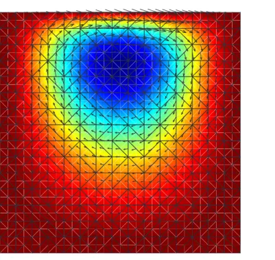
The cavity domain consists of a unit length square. The flow kinematics is computed in the mesh depicted in figure 4 assuming a Newtonian solvent fluid with unit viscosity. The fluid velocity is prescribed on the cavity boundary, vanishing on the lower and lateral walls, and taking a parabolic profile on the upper wall (avoiding velocity discontinuities at the upper corners):
v(x, y = 1) = µ 16x2(1 − x)2V max 0 ¶ (59) where Vmax was set to Vmax = 10Dr.
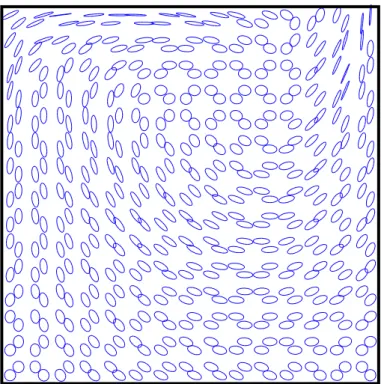
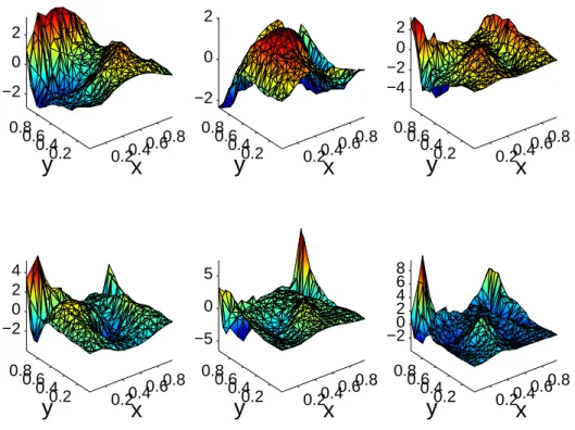
Figure 4 depicts the computed velocity field as well as the reconstructed stream function Ξ(x). The orientation field is depicted in figure 5. In that figure the ellipsoids axes are related to the second order orientation tensor eigenvalues, that represent the probability of finding the fiber aligned on the direction of the associated eigenvector.
6 Advanced strategies: techniques based on model reduction
In the previous section the driven cavity flow problem was simulated by using an integration by characteristics (in the physical space) coupled with a standard SUPG finite element discretization in the conformation space. However, despite the right scheme accuracy, the proposed algorithm requires significant computing efforts. By this reason, we propose in this section some new advanced model reduction strategies, that were successfully applied in some of our former works for simulating complex fluid flow problems.
The first strategy consists in computing the solution along one or several flow stream-lines, and then extract the most significant characteristics of the solution in the conforma-tion space by applying the proper orthogonal decomposiconforma-tion. This technique was success-fully applied in [4] [41] and throughout the present section will be summarized and applied for solving the computing the fluid microstructure in the flow cavity problem.
The second strategy that we are analyzing lies in the application of a separated repre-sentation of the trial and test fields involved in the variational formulation related to the suspension microstructural state. Separated representations and tensor product approxima-tion basis were successfully used in some of our former works (see [5] [6] and the references therein) for solving different kinetic theory models arising in complex fluids modelling.
In the next paragraphs we are summarizing the basic ideas related to the proper orthog-onal decomposition that will be then applied for solving the kinetic theory model related to the microstructural state of the fiber suspension in a driven cavity flow.
6.1 The proper orthogonal decomposition revisited
We assume that the evolution of a certain field T (x, t) is known. For the sake of simplicity we assume in what follows that this field is scalar, but all the developments can be extended to general tensorial fields. In practical applications, this field is defined at the nodes of a spatial mesh xi and for some times tm = m × ∆t, with i ∈ [1, · · · , N ] and m ∈ [0, · · · P ]. We introduce the notation T (xi, tm) = Tm(xi) ≡ Tim(tm). Tmdefines the vector containing the nodal degrees of freedom at time tm. The main idea of the proper orthogonal decomposition is to obtain the most typical or characteristic structure φ(x) among these Tm(x), ∀m. The maximization of: α = Pm=P m=1 h Pi=N i=1 φ(xi)Tm(xi) i2 Pi=N i=1(φ(xi))2 (60)
leads to: m=PX m=1 h³i=NX i=1 ˜ φ(xi)Tm(xi) ´³j=NX j=1 φ(xj)Tm(xj) ´i = α i=NX i=1 ˜ φ(xi)φ(xi); ∀ ˜φ (61) which can be rewritten in the form
i=N X i=1 (j=N X j=1 hm=PX m=1 Tm(xi)Tm(xj)φ(xj) i ˜ φ(xi) ) = α i=NX i=1 ˜ φ(xi)φ(xi); ∀ ˜φ (62) Defining the vector φ such that its i-component is φ(xi), Eq. (62) results in the eigen-value problem (63), whose eigenvectors related to the highest eigeneigen-values define the char-acteristic structure of Tm(x),
˜
φTc φ = α ˜φTφ; ∀ ˜φ ⇒ c φ = αφ (63)
where the two points correlation matrix is given by
cij = m=MX m=1 Tm(xi)Tm(xj) ⇔ c = m=MX m=1 Tm(Tm)T (64)
which is symmetric and positive definite. If we define the matrix Q containing the discrete field history: Q = T1 1 T12 · · · T1P T1 2 T22 · · · T2P .. . ... . .. ... T1 N TN2 · · · TNP (65)
then it is easy to verify that the matrix c in Eq. (63) results
c = Q QT (66)
6.1.1 A posteriori reduced modelling.
To define a reduced model we start solving the eigenvalue problem defined by Eq. (63) and then selecting the eigenfunctions φk associated with the eigenvalues belonging to the interval defined by the highest eigenvalue and that value divided by a large enough value (108 in our simulations). In practice n is much lower than N . Now, we could try to use these n eigenfunctions φk for approximating the solution Tm(x), ∀m. For this purpose we need to define the matrix B = [φ1· · · φn]
B = φ1(x1) φ2(x1) · · · φn(x1) φ1(x2) φ2(x2) · · · φn(x2) .. . ... . .. ... φ1(xN) φ2(xN) · · · φn(xN) (67)
Now, if we consider the linear system of equations resulting from the semi-implicit discretization of a generic parabolic partial differential equation:
expressing Tm+1= i=n X i=1 ζim+1 φi = B ζm+1 (69) equation (68) results Gm Tm+1 = Hm⇒ Gm B ζm+1 = Hm (70)
and by multiplying both terms by BT we obtain
BTGm B ζm+1 = BTHm (71)
where the size of BTGm B is n × n, instead N × N . When n ¿ N , as is the case in numerous physical models, the solution of Eq. (71) is preferred because its reduced size.
Remark 4. Equation (71) can be also deduced by introducing the approximation (69)
into the Galerkin variational form related to the partial differential equation. If trial and test functions in the vartiational formulation of a parabolic partial differential equation are approximated using the form (69) then Eq. (71) is easily deduced.
Remark 5. An alternative technique to reduce the size of the eigenvalue problem lies in
the application of the snapshot proper orthogonal decomposition. This technique is based on finding the significant modes from the application of the POD, but assuming that those modes can be written as a linear combination of the M snapshots that were used to define the decomposition. The main advantage of this strategy is that theses modes result from the eigenproblem defined by
¡
QTQ¢Υ = λ Υ (72)
whose size is P × P instead of N × N . Only the eigenvectors related to large enough eigenvalues are retained. From these eigenvectors the reduced approximation functions are computed using the fact that these functions are linear combination of the snapshots, i.e.:
φi = Q Υi (73)
Remark 6. In the previous analysis the reduced basis was built from the computed unknown
field evolution that was carried out solving the discrete evolution problem. Thus, one could ask about the interest of a such approach. There are two kind of approaches widely considered. The first approach consists in solving the non-reduced model in a short time interval, allowing the extraction of the characteristic functions and then the definition of the reduced approximation basis that is then used to perform the solution of the reduced evolution model in larger time intervals with the associated computing time savings. The other approach consists in solving the non-reduced model in the whole time interval, whose solution allows defining the reduced approximation basis that then could be used for solving ”similar” models, as the ones that involve for example slight variations in some material parameters or in the boundary conditions. Some recent advances in such approaches can be found in [36], [31], [39], [40], [41] [9], [13], [25] and the references therein.
6.1.2 Towards and adaptive strategy: Enriching the approximation basis.
Obviously, accurate simulations require an error evaluation as well as the possibility of adapting the approximation basis by introducing new functions able to describe the solution features. Ryckelynck proposed in [39] an adaptive procedure, able to construct or enrich the reduced approximation basis. For this purpose, he proposed to enrich the reduced approximation basis by adding some Krylov subspaces generated by the equation residual. Despite the fact that this enrichment tends to increases the number of approximation function, when it is combined with a POD decomposition that continuously reduces this number, the size of the problems is quickly stabilized. This strategy, which was successfully used in [4] as well as in [41], is summarized in the present section.
We assume the solution accurately described in the interval ]0, ts] by using the reduced basis B. Now, the solution evolution is performed in the time interval ]ts, ts+1] solving Eq. (71) making use of the reduced approximation basis defined by matrix B:
ζm+1 = ¡BTGm B¢−1BTHm (74)
When time ts+1 is reached, a control step is performed in order to evaluate the accuracy of the solution computed using the reduced basis. The control step is performed only at the end of each time interval.
We assume that ts+1− ts = M × ∆t and consequently the residual at ts+1, RM, can be computed from
RM = GM −1 B ζM − HM −1 (75)
If the norm of the residual is small enough kRMk < ² kB ζMk (being ² a small enough parameter) the computed solution can be assumed as good, and the time integration goes on in ]ts+1, ts+2] using Eq. (74) without changing the reduced approximation basis.
On the contrary, if kRMk ≥ ² kB ζMk, the approximation must be improved. For this purpose, we propose to enrich the reduced approximation basis by introducing the just computed residual (or some Krylov’s subspaces generated by the residual, as proposed in [39]):
B ← [B RM] (76)
and now, the evolution is recomputed in the ]ts, ts+1] using Eq. (74) with the just updated reduced basis B. When the convergence criterion is satisfied (i.e. kRMk < ² kB ζMk) we apply a POD on the entire past history ]0, ts+1] for defining the reduced basis able to represent all the past evolution of the unknown field, which results in an updated B that can be considered as the optimal reduced basis to describe the evolution of the unknown field in ]0, ts+1]. Using the just updated reduced basis B the time evolution given by Eq. (74) is performed in ]ts+1, ts+2] and the solution accuracy is checked at t = ts+2.
If a basis enrichment was needed at the end of the previous time interval, at t = ts+1, then the length of the present time interval is reduced according to ts+2−ts+1 = (ts+1−ts)/2, and if not enrichment was needed, then the time interval length is increased according to
ts+2− ts+1 = 2 (ts+1− ts) (see [4] for more details on the time interval length adaptation). The enrichment tends to increase the size of the reduced basis, but the POD reduces its size. The combination of both procedures allows to stabilize the size of the model as we noticed in some of our former works [4].
6.2 Building-up the reduced kinetic theory model of the fiber suspension We consider an arbitrary point in the flow domain, at which an isotropic fiber distribution is assumed. Now, the evolution of the orientation distribution is computed along the asso-ciated streamline using the ”a posteriori” model reduction algorithm just proposed applied on Eq. (33), and the solution at different times tiare stoked in matrix Σ, whose i-th column contains the orientation distribution at each node used to discretize the conformation space at time ti.
Now, we can extract the most significant information related to the orientation distri-bution evolution by applying a proper orthogonal decomposition. For this purpose we solve the eigenproblem defined by
(ΣΣT) V = λ V (77)
which leads to Nccouples Vj, λj(Ncbeing the number of nodes used in the discretization of the conformation space). Now, only the must significant eigenvectors are retained V1· · · Vr, with r << Nc according to the criterion:
λi
max λi > 10
−4 (78)
Then, a good approximation basis can be built from these significant eigenvectors: Ψ = Ψ0+
n X i=1
Viξi (79)
which can be written in a matrix compact form as:
Ψ = Bξ (80)
that is inserted into the discrete form of the Fokker-Planck equation BTK1B | {z } e K1 ˙ξ + BTK 2B | {z } e K2 ξ = 0 (81)
that defines a linear system of size r instead Nc.
6.2.1 Results
To conclude about the accuracy of the just proposed reduced modelling we depict in figure 6 the error associated with the second order orientation tensor, defined in Eq. (5), which is computed at each element of the flow domain mesh by:
Ee= Tr((ae− aered)2) (82)
where aeis the solution computed at element Ω
eusing the global approximation basis, and ae
redthe one computed from the reduced model than only contains around 10 approximation functions.
We can also define the mean error from:
E =
PNe e=1Ee
that results for the error depicted in figure 6: E = 1.3 × 10⁻⁵.
We can notice the excellent accuracy obtained using the reduced modelling, despite the significant reduction of the CPU time. The problem solution using model reduction is 600 times faster.
The solution can be improved by considering different flow streamlines (or the same with different initial conditions), which lead to different reduced bases: V(j)i , i ≤ r(j), where (j) refers to the different computed reduced bases. Now, from these bases we can extract a global one V1· · · VR by adding to the first one V1· · · V(1)r only the vectors contained in the other reduced bases whose projection on the previous updated basis is lower than a certain tolerance (to maximize their linear independence).
Thus, when in the flow just analyzed another trajectory closer to the flow domain walls is considered, the solution is improved as we can notice in figure 7, being the mean error in this case E = 8 × 10⁻⁸ (using 15 approximation functions in the reduced basis).
6.3 Empirical natural closure relation
As was indicated in the first section, the description of the microstructure state by means of the moments of the orientation distribution function (orientation tensors) is suitable from a computational point of view because the important CPU times savings that its use implies, but this approach requires the introduction of a closure relation. Today, it is widely accepted that the use of such a closure relation can have a significant, and sometimes unpredictable, impact on the computed solution. Numerous closure relations have been proposed, but there is not a universal or exact relation to be used in any flow conditions.
In this section we are defining an empirical and local natural closure relation that can be adapted locally to each flow conditions. This procedure was deeply described in [38] and its main ideas are revisited in the present section.
6.3.1 Fundamentals
Any closure approximation of the fourth order orientation tensor can be written using the Caley-Hamilton theorem as well as partial normalization and symmetry [22] in the general form: A =Pi=6i=1Biβi in 3D A =Pi=3i=1Biβi in 2D (84) where the different fourth order tensors involved in the former expression write:
B1 = S(I ⊗ I) B2 = S(I ⊗ a) B3 = S(a ⊗ a) B4 = S(I ⊗ a2) B5 = S(a ⊗ a2) B6 = S(a2⊗ a2) (85)
where S( ) refers to the symmetric component.
Now, taking into account the normalization conditions, we obtain the relations that the coefficients βi verify in the three-dimensional case:
10 1 00 7 2 0 0 4 ββ12 β3 = 1 − 2D0 1 − 6D4P 4(P − D)4P 7 5 2(3 − 4D) ββ45 β6 + 06 0 (86)
and in two-dimensional: µ 8 1 0 1 ¶ µ β1 β2 ¶ = µ 4P −1 ¶ β3+ µ 0 1 ¶ (87) where P = det(a) and D = 12¡1 − Tr(a2)¢.
In the general case, we can write Eqs. (86) and (87) in the matrix form:
f βu = gβd+ h (88)
Thus, the matrix form of Eq. (84) becomes A = Wβ = W µ βu βd ¶ = W µ f−1g I ¶ βd+ W µ f−1h 0 ¶ = ˜Wβd+ ˘W (89)
where now A denotes de vector form of the fourth order orientation tensor.
Now, considering the former equation for the n couples of tensor (Ai, ai) extracted via the Karhunen-Lo`eve decomposition from the most significant distribution functions (obtained by solving the Fokker-Planck equation along some streamlines), one could be interested in determining the optimal value of βd, as originally considered in [22] to derive the natural closure relation. However, in [22], authors considered only the orientation distribution related to an initial isotropic distribution of infinite slender fibers, without diffusion effects, immersed in a simple shear flow.
6.3.2 Computing the local natural closure relation
For computing the unknown beta coefficients we proceed by using a moving least square technique. For this purpose we define the approximation error
J(a, βd) = n X i=1 δ²( k a − ai k ) γi h Ai− ˜Wiβd− ˘Wi i2 (90) where the weighting coefficient γi scales with the value of the eigenvalue related to the eigenfunction that served for computing tensors Ai and ai. The window function δ²( ) is introduced for increasing the weight of closer couples in the error expression. In our simulations we have considered the following window function:
δ²(d) = δ¡d²¢ ² with δ µ d ² ¶ = e −(d ²) 2 √ π (91)
In the case of ² → ∞ we can write δ² = √1π. Thus, J becomes independent of a and the expression (90) reduces to the usual global least squares. In this case the vector βd does not require to be updated, which results in significant computing time savings.
In the general case, the minimization of the functional (90) leads to:
∂J ∂βd = 0 = 2 n X i=1 δ²( k a − aik ) γiW˜iT h Ai− ˜Wiβd− ˘Wi i (92) which results in:
" n X i=1 δ²( k a − ai k ) γiW˜ Ti W˜ i # βd= n X i=1 δ²( k a − aik ) γiW˜iT h Ai− ˘Wi i (93)
or βd= " n X i=1 δ²( k a − ai k ) γiW˜ Ti W˜ i #−1 n X i=1 δ²( k a − aik ) γiW˜iT h Ai− ˘Wi i (94) that allows computing for each value of a the coefficients of the empirical closure relation
βd, from which one could compute βu from Eq. (88). Both, βdand βu, define completely the closure relation:
A = W(a)β(a) (95)
The use of the just described procedure only requires the extraction of the couples (Ai, ai)
6.3.3 Extracting the characteristic structure of the orientation distribution
For extracting the characteristic structure of the orientation distribution one could solve the Fokker-Planck equation (that does not involve any closure relation) by using one of the techniques previously described, along some flow streamlines.
Thus, one could consider different snapshots of the orientation distribution (stored in the matrix Σ), from which the characteristic structure of the solution evolution could be determined by direct application of the Karhunen-Lo`eve decomposition.
Now, we could define the couples (Ai, ai) using three different strategies:
1. The simplest alternative lies in applying the Karhunen-Lo`eve decomposition to the solution history stored in Σ. Obviously, the resulting eigenfunctions do not have a fully physical meaning, and therefore they are not strictly positives. Thus, if we compute the second and fourth order moments (Ai, ai) associated with the model eigenfunctions, then these tensors have unusual properties (e.g. ai do not have a unit trace, ...). However, one could forget these ”conceptual difficulties” and apply the procedure described in the previous section to the couples (Ai, ai).
2. Other possibility to avoid these modes without a full physical meaning consists of as-suming that the orientation distribution can be written everywhere on the considered streamline as a linear combination of some orientation distributions (snapshots), for example, those were used for applying the Karhunen-Lo`eve decomposition. In order to avoid the consideration of two distributions too close, one could start with the ini-tial distribution, adding a new distribution to the reduced approximation basis only when it is far enough from all the functions defining the reduced approximation basis. The advantage of this approach is that all the modes used for approximating the ori-entation distribution evolutions are real physical distributions and consequently the associated second order orientation tensors are perfectly defined from all points of view.
3. Finally, one could consider a third possibility related to the snapshot Karhunen-Lo`eve decomposition. This technique is based on finding the significant modes from the application of the Karhunen-Lo`eve decomposition, but assuming that those modes can be written as a linear combination of the Nsnapsnapshots that were used to define the decomposition. The main advantage of this strategy derives from the fact that it is easy to prove that theses modes result from the eigenproblem defined by
¡
whose size is Nsnap×Nsnapinstead of Nc×Nc(Ncbeing the number of degrees of free-dom used to define the approximation in the configuration space – the one related to the orientation –), and where only the eigenvectors Υi related to large enough eigen-values ˜λi are retained. From those eigenvectors the reduced approximation modes are computed using the fact that those modes are linear combination of the snapshots, i.e.:
Vi= ΣΥi (97)
6.3.4 Numerical tests
In this section we are addressing two rheometric simple flows as well as the complex driven cavity flow problem.
• Simple shear flow.
Firstly, we consider the 2D flow defined by the velocity field vT = ( ˙γy, 0) with ˙γ = 1. The fiber aspect ratio was adjusted to have k = 0.8, being the diffusion coefficient
Dr= 0.1.
The 2D orientation distribution is computed using a stabilized SUPG finite elements discretization in the conformation space, on the mesh associated with the conforma-tion space that consists of 200 nodes uniformly distributed in [0, 2π[.
When the Fokker-Plank equation is integrated along a trajectory from the isotropic initial state until reaching the steady state characterized by a small enough variation between two consecutive time steps, that is:
k Ψ(tn+1) − Ψ(tn) k ≤ 10−6 k Ψ(t1) − Ψ(t0) k (98)
The three procedures described in the previous sections are applied to compute the characteristic structure of the solution (orientation distribution) evolution, that will be then used to compute the couples (Ai, ai). The functions defining the reduced ap-proximation basis obtained by applying the three procedures are depicted in Figs. 8, 9 and 10 respectively. We can notice that only 5 functions are needed for approximating accurately the evolution of Ψ.
In order to compare these different strategies, we have computed the reference second order orientation tensor from the resolution of the Fokker-Planck equation, and then the different orientation tensors using the closures proposed in the previous section. The reference and approximated second order orientation tensors were compared at different times, for different values of the diffusion coefficients, using the following error measure:
E = k aref − aappr k (99)
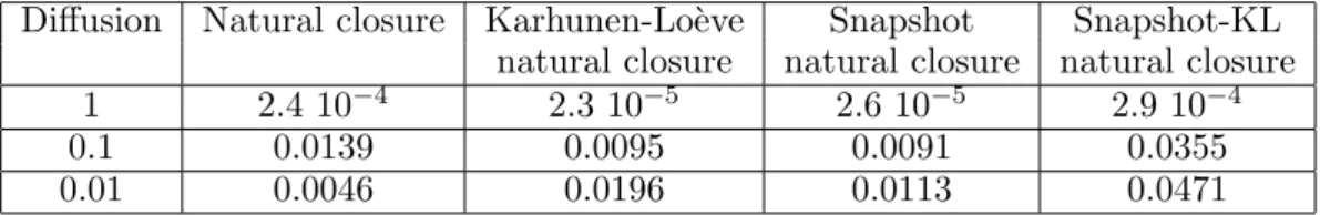
The table that follows groups the different computed errors at the end of the evolution process. We can notice that when the diffusion coefficient is small enough the standard natural closure relation works perfectly because we are close to the hypothesis under which it was derived. However, when the diffusion coefficient is increased, the solution accuracy is degraded. On the other hand, the adaptive natural closure that we have defined works perfectly for any diffusion coefficient, except for the too small values
that induce numerical difficulties in the finite element discretization of the Fokker-Planck equation in the conformation space. We must mention that due to the fact that the Karhunen-Lo`eve and the Snapshot Karhunen-Lo`eve natural closures are built from modes (approximation functions) that have not a full physical meaning we have preferred using a global least square technique. Moreover, the global least squares fitting can be applied without a significant impact on the solution accuracy and with a considerable computing time reduction.
Diffusion Natural closure Karhunen-Lo`eve Snapshot Snapshot-KL natural closure natural closure natural closure
1 2.4 10−4 2.3 10−5 2.6 10−5 2.9 10−4
0.1 0.0139 0.0095 0.0091 0.0355
0.01 0.0046 0.0196 0.0113 0.0471
Now, we analyze the effect of moving least square by considering different values of ² for Dr = 0.1, using the snapshot natural closure. The table that follows summarize the results.
² = ∞ ² = 1 ² = 0.3 ² = 0.1 ² = 0.05 ² = 0.03 ² = 0.01
0.091 0.091 0.091 0.093 0.096 0.097 0.097
There is no significative differences between the global and local (moving) least squares. Because the global least squares is suitable from the computational point of view (as was indicated above) in that follows we will consider ² = ∞.
• Extensional flow.
We consider a 2D extensional flow whose kinematics is defined by gradv = µ ˙² 0 0 − ˙² ¶ (100) being the elongation rate ˙² = 1. The fiber suspension is characterized by fibers whose shape factor leads to k = 0.8. The orientation distribution (assumed 2D) is discretized using the SUPG finite element method on the mesh associated with the conformation space that consists of 200 nodes uniformly distributed in [0, 2π[.
Figure 11 depicts the time evolution of the error defined in Eq. (99) for Dr = 0.01 and Dr = 0.1 where only the snapshot natural closure is compared with the standard natural one. We can notice the superior accuracy of the empirical snapshot natural closure for both diffusion coefficients.
The table that follows groups the errors, computed at the end of the time simulation, computed by using the different natural closure relations. Again, the best results are obtained by using the empirical snapshot natural closure.
Diffusion Natural closure Karhunen-Lo`eve Snapshot Snapshot-KL natural closure natural closure natural closure
1 2.1 10−3 2 10−4 1.3 10−4 2.5 10−3
0.1 0.0582 0.0439 0.0055 0.6719
• The driven cavity flow problem.
Finally, we consider the complex flow generated in a driven cavity that involves a short fiber suspension characterized by the same material parameters that in the pre-vious tests. The velocity is prescribed on the domain boundary according to: v(x = 0, y) = 0, v(x = 1, y) = 0, v(x, y = 0) = 0 and v(x, y = 1) = (16vmaxx2(1 − x)2, 0). The velocity field is then solved by assuming a Newtonian behavior and by applying a standard mixed finite element formulation where the velocity and pressure approx-imations verify the LBB stability condition. The Fokker-Planck equation governing the evolution of the fiber orientation distribution function is then solved along some closed streamlines, where the periodicity condition of that distribution function was imposed as described in Ammar and Chinesta [3]. From the computed orientation distribution function, the characteristic modes are extracted by using the technique previously described based on the application of the Karhunen-Lo`eve decomposition, allowing to fit the empirical snapshot natural closure strategy previously introduced. Now, the evolution equation associated with the second order orientation tensor is solved by assuming different closure relations: linear, quadratic, hybrid, natural and the empirical natural one.
If the Fokker-Planck equation is solved in the whole domain considering a fine enough mesh, the fiber distribution function can be computed everywhere without address-ing any closure relation. Thus, the second order orientation tensor related to the just computed distribution function can be used as reference solution for comparison purposes.
The error between the computed second order orientation tensor (computed by using the most usual closure relations) and the reference solution coming from the solution of the Fokker-Planck equation is reported in the following table, where we can notice that the empirical snapshot natural closure remains again superior.
Diffusion Linear Quadratic Hybrid Natural Snapshot
1 0.0031 0.0704 0.0062 0.0019 0.0008
0.1 0.1992 0.1516 0.08 0.0353 0.0289
0.01 1.1286 0.1452 0.1048 0.1216 0.1126
7 Advanced strategies: techniques based on separated representations
In general, models arising from the kinetic theory descriptions here defined in moderate or even highly multidimensional spaces that include the physical space, time and the confor-mation coordinates whose number depends on the level of richness of the physical model. Thus, the dimension of models ranges from 6D for the simplest kinetic theory models de-scribing for example the fiber orientation to thousands or millions of dimensions for those arising from the kinetic theory of systems involving macromolecules or the ones coming from quantum chemistry in which the dimension of the space in which the wavefunction is defined scales linearly with the number of particles involved in the system.
The solution of models like the one just described needs for new strategies, because the standard ones exhibit curse of dimensionality. Some strategies have been recently proposed for solving models defined in multi-dimensional spaces. The sparse grid techniques [12] are one of the most popular, but separated representations were also used for solving the models encountered in quantum mechanics (Hartree-Fock and post-Hartree-Fock techniques).
The sparse grid are restricted (at least in our knowledge) for treating models involving up to twenty dimensions [1]. On the other hand, separated representations like the one considered in the multi-configuration-self-consistent-fields (MCSCF), fix a priori the number